An optical parallel architecture for the random-iteration algorithm to decode a fractal image by use of iterated-function system IFS codes is proposed. The code ...
Random-iteration algorithm-based optical parallel architecture for fractal-image decoding by use of iterated-function system codes Hsuan T. Chang and Chung J. Kuo
An optical parallel architecture for the random-iteration algorithm to decode a fractal image by use of iterated-function system ~IFS! codes is proposed. The code value is first converted into transmittance in film or a spatial light modulator in the optical part of the system. With an optical-to-electrical converter, electrical-to-optical converter, and some electronic circuits for addition and delay, we can perform the contractive affine transformation ~CAT! denoted in IFS codes. In the proposed decoding architecture all CAT’s generate points ~image pixels! in parallel, and these points then are joined for display purposes. Therefore the decoding speed is improved greatly compared with existing serial-decoding architectures. In addition, an error and stability analysis that considers nonperfect elements is presented for the proposed optical system. Finally, simulation results are given to validate the proposed architecture. © 1998 Optical Society of America OCIS codes: 250.0250, 110.6980.
1. Introduction
Fractal techniques for image coding have recently attracted a great deal of attention. Barnsley1,2 found that a finite set of specific contractive transform functions of an iterated-function system ~IFS! can be used to generate a fractal image. An IFS can achieve high data compression, and its decoding algorithms are simple.3 However, it is computation intensive for encoding and decoding fractal images. Clearly this precludes the use of such a method for real-time applications. On the other hand, the parallelism and high-speed nature of optics are very suitable for this application. In this paper we propose an optical parallel-decoding architecture that can rapidly generate a fractal image. Recently some methods4 – 6 were proposed to solve the inverse problem of the encoding procedure, and some decoding algorithms7,8 were provided to speed When this study was performed, the authors were with the Signal and Media ~SAM! Laboratory, Department of Electrical Engineering, National Chung Cheng University, Chiayi 62107, Taiwan. H. T. Chang is now with the Department of Electronic Engineering, Chien Kuo College of Technology and Commerce, Changhua 500, Taiwan. Received 21 October 1996; revised manuscript received 16 June 1997. 0003-6935y98y081310-09$10.00y0 © 1998 Optical Society of America 1310
APPLIED OPTICS y Vol. 37, No. 8 y 10 March 1998
up the decoding procedure. On the other hand, two optical architectures have been proposed and implemented9,10 to show the parallelism and high-speed properties of optics. Tanida et al.9 presented an optical fractal synthesizer ~OFS! to generate fractal images from IFS’s with a deterministic algorithm. With this OFS technique all the points in an image shown on a CRT are duplicated and then transformed optically with one of the affine transformations. The transformed images are combined into a single image and fed back through a CCD camera for the next iteration. After a sufficient number of iterations a fractal image is obtained, and its shape is determined by the characteristics of the optical affine transformations. This technique solves the discontinuity problem caused by the rotation, magnification, or reduction of a digital image. However, this OFS can decode only a fractal image that consists of a regular pattern or texture because the affine transformations in this architecture operate with equal probability. Also, the decoding speed is limited by the CCD camera used in the OFS, and the image quality of the generated fractal images is determined by the physical resolution of the optical system. A serial optical architecture based on the randomiteration algorithm for decoding IFS codes was proposed in Ref. 10 to solve the above problems. Instead of electronic calculations, a high-speed optical architecture is proposed to implement the contractive affine
transformation ~CAT!. This architecture can decode complicated fractal images. The resolution of the generated fractal images is limited by only the resolution of the display device. Although optics are used to perform the CAT operation, the fractal image is decoded point by point, sequentially. Apparently the parallel-processing characteristics of optics are not fully employed. Here we propose a new optical parallel architecture that can generate the decoded points in parallel, thus greatly improving the decoding speed. Furthermore, error and stability analyses of practical applications are also performed for the proposed optical system. The organization of this paper is as follows: In Section 2 we first review the IFS that employs CAT’s and the random-iteration algorithm. Then a fully parallel algorithm for the proposed optical system is described in Section 3. The proposed optical parallel-decoding architecture is presented in Section 4. We give the error and stability analyses for our optical implementation in Section 5. Section 6 demonstrates our simulation results, and finally we conclude in Section 7. 2. Review of Iterated-Function Systems A.
Contractive Affine Transformation
The IFS theory is an extension of classical geometry. It uses CAT’s to express relations between different parts of an image. Affine transformation can be described as a combination of rotation, scaling, and translation of the coordinate axes in an n-dimensional space. The general form of a CAT is
HF GJ F G
W
x y
5A
F GF G F G
x a 1b5 y c
b x e 1 , d y f
(1)
where the coefficients a, b, c, d, e, and f are real numbers, a–d are within the range 21–1, and udet~A!u 5 uad 2 bcu , 1,
(2)
where det~A! represents the determinant of the matrix A. These coefficients are used to describe rotation, scaling, and translation. Because fractal images have self-similarity, we can find N CAT’s, $Wi , i 5 1, 2, . . . , N%, such that N
F 5 ø Wi ~F!,
(3)
i51
where F is a fractal image and Wi ~F! is a subimage given by the CAT. An IFS consists of a metric space ~R, d! together with a finite set of contractive mapping ~i.e., CAT’s! Wi : R 3 R, with contractivity factors si for i 5 1, 2, . . . , N, respectively. The notation for the IFS is $R 3 R; Wi , i 5 1, 2, . . . , N%; its contractivity factor is s 5 max$si : i 5 1, 2, . . . , N%. Note that the contractivity factor s relates directly to the absolute value of the determinant of the matrix A and 0 # s , 1.
Table 1. IFS Codes for a Sierpinski Triangle
W
a
b
c
d
e
f
p
1 2 3
0.5 0.5 0.5
0 0 0
0 0 0
0.5 0.5 0.5
0 1 0.5
0 0 0.5
0.33 0.33 0.34
Here is an example ~a Sierpinski triangle! of an IFS with three transformations: W1 W2 W3
FG F FG F FG F
GF G F G GF G F G GF G F G
x 0.5 0.0 x 0 5 1 , y 0.0 0.5 y 0 x 0.5 0.0 x 1 5 1 , y 0.0 0.5 y 0
x 0.5 0.0 x 0.5 5 1 . y 0.0 0.5 y 0.5
Each transformation must also have an associated probability pi that determines its importance relative to the other transformations. In the present case we have p1, p2, and p3, and these probabilities must add up to 1 ~that is, p1 1 p2 1 p3 5 1!. Clearly, the above notation for an IFS is cumbersome. Table 1 expresses the same information in tabular form. Another example ~a fractal tree! of IFS codes is given in Table 2. Note that an IFS can contain any number of CAT’s. B.
Random-Iteration Algorithm
There are two basic decoding algorithms for IFS codes: a deterministic algorithm and the randomiteration ~probabilistic! algorithm. The randomiteration algorithm is frequently used to decode fractal images since it uses the property of probability corresponding to each CAT; hence the computational load can be reduced.3 The deterministic algorithm can be seen as a special case of the random-iteration algorithm since the probability of each CAT is the same. However, it is inefficient when the size of the subimage corresponding to each CAT is different. The random-iteration algorithm generates an image point by point, and the decoding speed is slow when the image size is large. Assume that the IFS codes are known. Then the random-iteration algorithm is summarized as follows: Step 1: An arbitrary initial point ~xt, yt! is chosen. Step 2: For t 5 0 to #itr, perform steps 3–5. Step 3: One of the CAT’s Wi , i 5 1, . . . , N, with a probability pi , is randomly selected. Step 4: Apply transformation Wi to the point ~xt, yt! to obtain ~xt11, yt11!. Step 5: Plot ~xt, yt! if t . 10. Table 2. IFS Codes for a Fractal Tree
W
a
b
c
d
e
f
p
1 2 3 4
0 0.1 0.42 0.42
0 0 20.42 0.42
0 0 0.42 20.42
0.5 0.1 0.42 0.42
0 0 0 0
0 0.2 0.2 0.2
0.05 0.15 0.4 0.4
10 March 1998 y Vol. 37, No. 8 y APPLIED OPTICS
1311
ated by the application of the feedback point to a randomly selected CAT. B.
Fig. 1. Block diagram of the proposed parallel-decoding algorithm.
In step 2, #itr indicates the number of points that the process repeatedly generates. By varying #itr, we can vary the density of the image, i.e., a denser image can be generated with a larger value of #itr. This algorithm generates the overall image point by point, in sequence, and is not suitable for parallel implementation. Moreover, an arbitrary initial point is used in this algorithm, so the points generated at the beginning are useless transient points and should be discarded. Therefore in Ref. 8 a parallel-decoding algorithm for IFS codes was proposed to improve the decoding speed and solve the problem of transient points. Here we present a new parallel-decoding algorithm in Section 3, and this algorithm is very suitable for hardware implementation. The proposed optical decoding architecture is constructed on the basis of this parallel algorithm. 3. Fully Parallel-Decoding Algorithm A.
Parallel Algorithm
A block diagram of the parallel-decoding algorithm is shown in Fig. 1. In this algorithm each CAT operates simultaneously, and the final output of the proposed architecture comprises the union points generated by each CAT. For avoiding the transient points during decoding, the initial points for each CAT can be given by the method shown in Ref. 8 or by the simplified method given in Ref. 11. We summarize the procedures of this parallel-decoding algorithm as follows: Step 1: An initial point ~xt, yt! is first determined. Apply ~xt, yt! to each Wi . Step 2: For t 5 0 to #itr, perform steps 3– 4 in parallel for each Wi . Step 3: Output the newly generated point and randomly feed this point back as the input to Wj ~i need not be equal to j!. Step 4: Plot the newly generated points. Step 5: The final image is the union of all results from N CAT’s Wi . For N CAT’s in an IFS there are N feedback paths. The feedback path for each newly generated point is randomly determined. After a random number is generated the corresponding feedback path for each point is selected. There are N ! ways to feed the output points back to W. The next point is gener1312
APPLIED OPTICS y Vol. 37, No. 8 y 10 March 1998
Two General Cases
The feedback and output controller shown in Fig. 1 determines the random feedback paths and the output frequencies of the generated points. If p1 5 p2 5 . . . 5 pN, the output frequency for the point generated by each CAT is the same. We thus achieve an N times faster decoding speed. When the probability for each CAT is not the same, we have to control the output frequency of the point generated by each CAT. Otherwise the fractal image generated will have different densities in each image subset. Two solutions are proposed to solve this problem. Assume that the maximum corresponding probability among all CAT’s is pmax, then the output frequency for the generated point of each Wi becomes pi ypmax pointsyiteration. For the CAT with a probability of pi less than pmax, the controller outputs the first kpi points of kpmax points, where k is the minimum constant such that both kpi and kpmax are integers. That is, there will be fewer than N output points in some iterations. Now the decoding speed is no longer N times the original speed, and it becomes N9 times faster, where N
N9 5
pi
(p i51
,
N9 # N.
(4)
max
Another solution is that we can add more modules for the CAT that possesses the higher probability. If the minimum probability among all CAT’s is pmin, then the number of modules required for each CAT is determined by @ pi ypmin#, where @. . .# denotes the operation of selecting the integer that is closest to pi ypmin. In this method the total number of CAT’s ˆ , is required, N N
ˆ 5 N
( i51
F G
pi , pmin
ˆ $ N. N
(5)
Since the output frequency of the generated point for ˆ times each CAT is 1, the decoding speed becomes N the serial-decoding speed. However, this method increases the total number of CAT’s and thus is not suitable for hardware implementation, especially for some i such that pi .. pmin. In fact, these two methods can be considered as two general cases. The first method can correctly decode a fractal image without the problem of nonuniformity; the second method, however, can decode an approximate fractal image when pi ypmin is not an integer. The example of the Sierpinski triangle is a special case because the probability for each CAT is ˆ 5 N in the same. That is, N9 5 N in Eq. ~3!, and N . . . Eq. ~4! if p1 5 p2 5 5 pN. 4. Proposed Optical Parallel-Decoding Architecture
The parallelism and high-speed nature of optics are very suitable for image processing. Therefore, instead of electronic calculations, a high-speed optical
Fig. 2. Single optical CAT module in the proposed parallel-decoding architecture.
architecture for performing the CAT operation is proposed to implement the parallel-decoding algorithm. A.
Optical Parallel-Decoding Architecture
Figure 2 shows the optical CAT module that is a basic unit in our parallel-decoding architecture. The fractal codes should be translated into transmittance signals at first. For implemention of Eq. ~1! the light intensity is used to represent the pixel position x, y within the range 0 –1, and the coefficients a–f are encoded by their corresponding transmittances Ta–Tf, which are in the range 0 –1. Then we rewrite Eq. ~1! as
HF GJ HF
W
x y
52
Ta Tc
GF G F GJ F GF G F G
Tb x T 1 e Td y Tf
2
1 1
1 x 1 2 , 1 y 1 (6)
where Tj 5 ~j 1 1!y2 and j 5 a–f. The terms inside the curly brackets on the right-hand side of Eq. ~6! are calculated by means of optics, while the others are calculated by electronics. The operation of this optical CAT module is based on the following facts: The result of the multiplication is the output light intensity when a light beam passes through a developed film @or a spatial light modulator ~SLM! with a given transmittance#. The result of the addition is obtained when two lightbeam intensities are simultaneously detected by a photodetector. Then, together with other optical CAT modules, we can decode a fractal image in parallel. Figure 3 shows a block diagram of the proposed parallel-decoding architecture. Each CAT in the IFS is implemented by an optical CAT module, as shown in Fig. 2. IFS codes a–f in each W are converted to transmittance signals Ta–Tf, respectively, with Eq. ~5! and are recorded in the films or appear in
the SLM’s. The advantage of using SLM’s is that we can modify their transmittances when we intend to decode other images. Note that the transmittance of the SLM need not be changed during the decoding process. Therefore the response time of the SLM is not a concern with respect to the decoding speed. After the IFS codes are translated into transmittances and appear on the film or in the SLM in each of the optical CAT modules, the iteration process begins. The optical CAT module receives the feedback point ~xi 9, yi 9! and outputs the point ~xi , yi ! at the next iteration. In each iteration, as soon as a probability is generated by the random-number generator, the feedback path for each output point is determined. When the probability for each CAT is the same, N output points are transmitted simultaneously to the display circuit, and the decoding speed is thus N times the decoding speed of the serial architecture. Otherwise, for the case of using N CAT modules, the output points for each CAT Wi are transmitted to the display circuit with a frequency of pi ypmax and the decoding speed is less than the speed for the equal-probability CAT. ˆ CAT modules in the proposed Another case of using N parallel architecture achieves the fastest speed by having full parallelism. However, it is not practical when pmax ,, pmin. For example, in Table 2 pmax 5 0.4 and pmin 5 0.05, and there will be 1 1 3 1 8 1 8 5 20 optical CAT modules in this parallel architecture, resulting in a system that is too large. B. Comparison with Previous Optical Serial-Decoding Architecture
An optical serial-decoding architecture was proposed in Ref. 10. In this architecture the fractal codes should be translated into transmittance signals on the electro-optic modulator ~EOM!.12 This can be 10 March 1998 y Vol. 37, No. 8 y APPLIED OPTICS
1313
Fig. 3. Block diagram of the proposed parallel-decoding architecture.
done by translation of the fractal codes into the modulation voltages ~Va–Vf ! of the EOM with10 Vz 5
SD
Vp z , sin21 p 2
z 5 a–f,
(7)
where Vp is the half-wave voltage that yields a phase retardation p in the EOM. The range of the modulation voltage is within 2Vpy2–Vpy2, and their corresponding transmittances are Ta–Tf, which are within the range 0 –1. Several drawbacks exist in this serial architecture. First, this is a serial architecture and the parallelism of optics is not exploited well. Furthermore, we have to convert the fractal codes into the voltages to be applied to the EOM, since the light intensity cannot be negative. The voltage must be changed during the iterations, and thus an additional electronic circuit for controlling the voltage is necessary. The decoding speed is slow, and the whole system is not compact enough. As for the proposed parallel architecture, the response time of the EOM is not important because the transmittance in each film–SLM is fixed during each iteration. Our proposed parallel architecture exploits the parallelism of optics well and solves the problems caused by the use of an EOM. Therefore we greatly improve the fractal image decoding speed. 5. Error and Stability Analyses
In practical applications of the proposed optical system it is necessary to consider the error or distortion caused by the nonperfect elements or devices, such as the mirror, beam splitter, and film–SLM. Therefore, here we examine the effects of errors on the optical CAT when the optical components are not perfect. The stability of image convergence is also discussed when errors happen. From the contraction-mapping theorem,1 a contraction mapping possesses exactly one fixed point when the determinant of the matrix A in Eq. ~1! satisfies the condition shown in expression ~2!. If the value 1314
APPLIED OPTICS y Vol. 37, No. 8 y 10 March 1998
uad 2 bcu is greater than one because of the errors mentioned above, the contraction-mapping theorem does not hold; hence the fixed point does not exist. Therefore the generated image may diverge. It is thus necessary to analyze the convergence property ~i.e., stability! when the above-mentioned errors occur. A.
Mirror Loss
As shown in Fig. 2, mirrors are used to reflect the optical signals so that the signals can pass through the film–SLM and arrive at the optical-to-electrical converter. If the mirror is not perfect, part of the input light will be scattered; hence the reflected light will be weaker than the input light. Here we introduce a loss factor a that denotes the percentage of the loss in optical signal power. Therefore, according to the architecture shown in Fig. 2, Eq. ~6! can be rewritten as
HF GJ HF GF G F F GF G F G
W
x y
52
2
Ta Tc
1 1
GJ
Tb x~1 2 a! Te 2 1 Td y~1 2 a! Tf ~1 2 a!
1 x 1 2 . 1 y 1
(8)
It is obvious that, as a is greater than zero, the term inside the curly brackets on the right-hand side will be modified, and the generated image will have errors. To analyze the stability in this case, we rewrite Eq. ~8! as
HF GJ F G F F
W
x y
5 Am
5
x 1 bm y
k~a 1 1! 2 1 k~c 1 1! 2 1
1
GF G
k2~b 1 1! 2 1 x k2~d 1 1! 2 1 y
G
e , k~ f 1 1! 2 1
(9)
Fig. 4. Decoded fractal images based on the random-iteration algorithm:
where k 5 1 2 a. is
The determinant of the matrix A m
det~A m! 5 k3~ad 2 bc! 1 k2~1 2 k!~b 2 d! 1 k~1 2 k!~1 1 k!~c 2 a!.
(10)
It is thus necessary to control the mirror loss such that udet~A m!u , 1. Otherwise, the fractal image will diverge, and the optical system becomes unstable. B.
Beam-Splitter Unbalance
Ideally, a 50:50 beam splitter splits an input optical signal into two equal halves. However, it is very difficult to achieve an exact 50:50 beam splitter. Therefore we assume that the 50:50 beam splitter performs a ~50 1 e!y~50 2 e! separation for the input light in a practical situation. On the basis of this assumption for the beam splitter in our optical system, the resultant transmittance becomes Tj 5 ~j 1 1!~0.5 1 b!,
j 5 a, c, e,
Tj 5 ~j 1 1!~0.5 2 b!,
j 5 b, d, f,
W
HF GJ F G F F x y
5 A bs
5
x 1 bbs y
a 1 2b~1 1 a! c 1 2b~1 1 c!
1
g~u! 5 L erf
G
GF G
2s
5
2L
p
uy~Î2s!
exp~2v2!dv, (14)
0
Tj 5
g# ~j! 1 1 , 2
j 5 a–f.
(15)
On the basis of a similar analysis of the mirror loss and the beam-splitter unbalance, the modified CAT is expressed by x y
5 An
F
x g# ~a! 1 bn 5 y g# ~c!
GF G F G
g# ~b! x g# ~e! 1 . g# ~d! y g# ~ f ! (16)
The determinant of the matrix A n becomes (12)
det~A n! 5 g# ~a! g# ~d! 2 g# ~b!g# ~c!,
(17)
and the convergence criterion for det~A n! is the same as that for det~A m! and det~A bs!.
det~A bs! 5 ad 2 bc 2 2b~a 2 b 1 c 2 d! 2 4b2 3 @~1 1 a!~1 1 d! 2 ~1 1 b!~1 1 c!#.
u
HF GJ F G
b 2 2b~1 1 b! x d 2 2b~1 1 d! y
e 1 2b~1 1 e! , f 2 2b~1 1 f !
SÎ D Î *
where erf~. . .! is the error function, L is the maximum value of the error function, and s is the degree of nonlinearity. The s value relates directly to the linearity of the transfer characteristics of the film–SLM. A highly linear film–SLM is obtained when s is much greater than one. Since the transmittance signal is within the range 0 –1, we let L be one and g# ~. . .! denotes that the range of g~. . .! has been normalized to the range 21–1. Now the relation between the coefficient and corresponding transmittance becomes
W
and the determinant of the matrix A bs is
(13)
Therefore the beam-splitter unbalance b should not make udet~A bs!u $ 1. C.
linearity of the transfer characteristic in the film– SLM should be considered in a practical system. Here we use the error-function limiter to model the device nonlinearity. Mathematically the errorfunction limiter is expressed as
(11)
where b 5 ey100 denotes the unbalanced quantity of the beam splitter. Substituting Eqs. ~11! into Eq. ~6!, we have
~a! Sierpinski triangle. ~b! Fractal tree.
Device Nonlinearity
In the proposed optical architecture the transform matrix coefficients are translated into transmittance signals based on linear mapping. However, the non-
6. Simulation Results
If we consider the original random-iteration algorithm, the decoded fractal images corresponding to the IFS codes in Tables 1 and 2 are shown in Figs. 4~a! and 4~b!, respectively. Here we let #itr equal 9000. From the computer simulation of the Sierpinski triangle for the proposed architecture we obtain the decoded points of each CAT, and their union image is shown in Fig. 5. Therefore we need only 3000 10 March 1998 y Vol. 37, No. 8 y APPLIED OPTICS
1315
Fig. 5. ~a!–~c! Three subimages of the Sierpinski triangle generated by the three CAT’s. ~d! Their union result.
iterations by using this parallel-decoding architecture to obtain a Sierpinski-triangle image of 9000 points. On the other hand, only one randomnumber generator is necessary. And we can get the subimage for each CAT by just displaying the points generated by the corresponding CAT module. We can also understand how the encoding algorithm partitions the image F into several subimages. In this example, the decoding speed is N times faster than
Fig. 6. ~a!–~d! Four subimages of the fractal tree generated by the four CAT’s. ~e! Their union result. 1316
APPLIED OPTICS y Vol. 37, No. 8 y 10 March 1998
Fig. 7. Decoded fractal tree image with a different uniformity on each subimage.
the serial-decoding algorithm, while the required number of CAT’s is the same. On the other hand, only one random generator is required. Obviously, the proposed architecture not only improves the decoding speed but also helps us understand the image partition. The probability for each CAT in the example above is the same. Consider the example shown in Table 2, its CAT’s have different probabilities. If we employ frequency control for the output points we can obtain the decoded points for each CAT and their union images, as shown in Fig. 6. However, when the output frequency for each CAT is not well controlled, the result of the union image becomes that shown in Fig. 7. Comparing the image shown in Fig. 4~b!, we see that two subimages corresponding to Figs. 6~a! and 6~b! appear darker, and the other parts appear brighter. This is an undesirable decoded image because of its nonuni-
Fig. 8. Absolute value of the determinant of the matrix A affected by ~a! a mirror loss of a 5 0 –1, ~b! a beam-splitter unbalance of b 5 0 – 0.5, and ~c! a device nonlinearity of s 5 0.1–50. BS, beam splitter.
Fig. 9. Normalized error e% between the ideal image and the images affected by ~a! a mirror loss of a 5 0 – 0.01, ~b! a beamsplitter unbalance of b 5 0 – 0.01, and ~c! a device nonlinearity of s 5 1–50.
formity. Apparently the proposed architecture shows its novelty when solving the problem of nonequal probability in parallel architectures. The simulation results above were obtained on the basis of the assumption that all the elements used in the optical parts are ideal. However, it is necessary to consider that the optical elements are rarely perfect in practical applications. Therefore we performed the simulation on the basis of the error and stability analyses given in Section 5. First, the absolute value of the determinant of the new matrix is
examined. On the basis of Eq. ~10!, the absolute value of the determinant det~A m! for the mirror loss in the range 0 –1 is obtained and shown in Fig. 8~a!. As shown in this figure, expression ~2! is satisfied in the range 0 –1 for the mirror loss a, and we can expect that, even if a serious mirror loss happens, a fixed point for the contraction mapping still exists. For the case of beam-splitter unbalance, the corresponding determinant is determined by Eq. ~13!. As shown in Fig. 8~b!, the absolute value of the determinant det~A bs! is smaller than one except for the extreme case that the beam-splitter unbalance b is 0.5. Therefore a fixed point still exists in this case. Finally, the absolute value of the determinant det~A n! for the device nonlinearity is calculated with Eq. ~17!. As the nonlinearity s is less than 0.1, the absolute value of the determinant is equal to one and expression ~2! is not satisfied. To stabilize the system we should keep the device nonlinearity s higher than 0.1. In practice, the above error factors in the optical elements are small13 and are within the determined ranges. Therefore we simulate the decoded images while considering only the small error effects. Since the decoded image is binary, we measure the fidelity of the decoded image by using the Hamming distance. Ideally the decoded Sierpinski triangle image is within the area whose horizontal ~x! and vertical ~ y! sizes are 0 # x , 2 and 0 # y , 1, respectively. Since the decoded image may be enlarged or contracted when the error occurs, we therefore normalize the error image such that it has the same size as the ideal image to calculate the Hamming distance. If the pixel is black, we assign the pixel a value of 0. Otherwise, we assign a value of 1
Fig. 10. Examples of the degraded images under ~a! a mirror loss of a 5 1%, ~b! a beam-splitter unbalance of b 5 0.5%, ~c! a device nonlinearity of s 5 2, and ~d! the compounding effects of ~a!–~c!. 10 March 1998 y Vol. 37, No. 8 y APPLIED OPTICS
1317
for a white pixel in a binary image. The Hamming distance H between two binary images F1 and F2 is defined as H5
(
uF1~i, j! 2 F2~i, j!u,
(18)
0#i, j,512
where F~i, j! denotes the ~i, j!th pixel in the image F. We next measure the normalized error ε% of the Hamming distance between the distorted and the ideal images, which is defined as ε% 5
H 3 100%. 5122
(19)
Figure 9 shows the normalized error ε% of the Hamming distance for the following cases14: ~a! a mirror loss of a 5 0 – 0.01, ~b! a beam-splitter unbalance of b 5 0 – 0.01, and ~c! a device nonlinearity of s 5 1;50. The error effect owing to the mirror loss is more obvious than that owing to the beam-splitter unbalance because the optical signals emitted from the electrical-to-optical converter pass through one beam splitter but are reflected by two mirrors. In the case of device nonlinearity the normalized error increases rapidly as s , 5 since the nonlinearity increases rapidly. On the other hand, when the film–SLM has high linearity, for example, s . 20, the normalized error is small and the decoded image is close to the ideal one. Here we demonstrate some examples of the degraded images shown in Fig. 10. In Fig. 10~a! the image is obtained by substitution of the mirror loss value of a 5 0.01 into Eq. ~9!. One of the three subimages is separated from the other two subimages. If we substitute the value of the beam-splitter unbalance b 5 0.005 into Eq. ~12!, the simulated image is that shown in Fig. 10~b!. The image is more irregular, and the total size is enlarged. If the film–SLM nonlinearity s is 2, the decoded image is that shown in Fig. 10~c!. Three subimages overlap each other at their connecting corners, and the total size is enlarged too. Finally, the compounding effect of the three cases shown in Figs. 10~a!–10~c! is shown in Fig. 10~d!. 7. Conclusion
In this paper we have proposed a novel optical parallel architecture for decoding fractal images using IFS codes. The fractal codes are first converted to their corresponding transmittances, and then they are recorded in films or shown in SLM’s. Then the CAT operation is performed by use of the optical parts proposed for the architecture. With the output and feedback control for the image pixel generated by the CAT, the proposed architecture can decode a fractal image in parallel. Furthermore, our parallel architecture is capable of decoding a fractal image even
1318
APPLIED OPTICS y Vol. 37, No. 8 y 10 March 1998
when the probability for each CAT is different. For an IFS with N CAT’s, the computer-simulation result shows that the decoding speed of our parallel architecture is N times faster than that of the serial architecture when the probability for each CAT is the same. Therefore the speed for fractal-image decoding is greatly improved. The error and stability analyses for the proposed optical system was studied for practical applications. In future research we plan to set up experiments for the optical part of the system. Then a working prototype of the proposed architecture will be implemented for completeness. This research was partially supported by the National Science Council, Taiwan, under contract NSC 86-2221-E-194-009. The authors thank the anonymous reviewers for their valuable comments and suggestions. References and Note 1. M. Barnsley, Fractals Everywhere ~Academic, Boston, Mass., 1988!, Chap. 3. 2. M. F. Barnsley and A. Sloan, “A better way to compress image,” BYTE 13, 215–223 ~Jan. 1988!. 3. M. Barnsley and L. Hurd, Fractal Image Compression ~Peters, Wellesley, Mass., 1993!. 4. M. Kawamata, H. Kanbada, and T. Higuchi, “Determination of IFS codes using scale–space correlation functions,” Proceedings of the IEEE Workshop on Intelligent Signal Processing Communication Systems ~Institution of Electrical and Electronics Engineers, New York, 1992!, pp. 219 –233. 5. S. Pei, C. Tseng, and C. Lin, “Wavelet transform and scale space filtering of fractal images,” IEEE Trans. Image Process. 4, 682– 687 ~1995!. 6. R. Rinaldo and A. Zakhor, “Inverse and approximation problem for two-dimensional fractal sets,” IEEE Trans. Image Process. 3, 802– 820 ~1994!. 7. H. A. Cohen, “Deterministic scanning and hybrid algorithms for fast decoding of IFS encoded image sets,” in Proceedings of the IEEE 1992 International Conference on Acoustics, Speech, and Signal Processing ~Institute of Electrical and Electronics Engineers, New York, 1992!, Vol. 3, pp. 509 –512. 8. S. Pei, C. Tseng, and C. Lin, “A parallel decoding algorithm for IFS codes without transient behavior,” IEEE Trans. Image Process. 5, 411– 415 ~1996!. 9. J. Tanida, A. Uemoto, and Y. Ichioka, “Optical fractal synthesizer: concept and experimental verification,” Appl. Opt. 32, 653– 658 ~1993!. 10. H. T. Chang and C. J. Kuo, “An optical decoding architecture for the random iteration algorithm of iterated function system codes,” Opt. Rev. 1, 146 –149 ~1994!. 11. H. T. Chang and C. J. Kuo, “A fully parallel algorithm for fractal image decoding using IFS codes,” IEEE Trans. Image Process. ~to be published!. 12. A. Yariv and P. Yeh, Optical Wave in Crystals ~Wiley, New York, 1994!, pp. 241–243. 13. 1995y96 OptoSigma Catalog: Optics Opto-Mechanics ~OptoSigma Corporation, Santa Ana, Calif., 1995!. 14. The ranges of the mirror loss and the beam-splitter unbalance are chosen according to the data given in Ref. 13.