2010 European Wireless Conference
Random Matrix Processes: Quantifying Rates of Change in MIMO Systems Peter Smith
Matthew McKay
Andrea Giorgetti and Marco Chiani
Department of Electrical and Department of Electronic and DEIS, CSITECNR, University of Bologna Computer Engineering Computer Engineering, HKUST V.le Risorgimento 2, 40136 Bologna, ITALY University of Canterbury Clear Water Bay, Kowloon, Hong Kong Email: mchiani,agiorgetti @deis.unibo.it Christchurch, New Zealand Email:
[email protected] Email:
[email protected]
Abstract— The rates of change of a wide variety of MIMO metrics are evaluated by differentiating the relevant random processes. Moments, distributions and simplified representations are derived where possible for the resulting derivatives. Fundamental metrics such as the channel coefficients, channel correlation matrices and eigenvalues are considered in addition to performance metrics such as bit-error-rate and the condition number. The analysis presents a comprehensive framework for studying the time-varying nature of MIMO systems in independent Rayleigh fading and leads to insights into the relative rates of change of the various metrics. For example, we show that there is a difference of several orders of magnitude between the moderate rates of change of channel elements and eigenvalues and the extremely rapid variations of the channel condition number. The channel eigenvectors are also shown to experience rapid fluctuations.
I. I NTRODUCTION It is well known that temporal variation of the wireless channel has a variety of effects on system performance including channel estimation errors, imperfect transceiver processing due to outdated channel state information (CSI) and bursty error behaviour. For this reason, the study of temporal variation is well established in communications research from the pioneering work of Rice [1] on level crossing rates (LCRs) onwards. The advent of multiple-input multiple-output (MIMO) systems has made the situation more complex. Such systems are not driven by individual channel coefficients but by time-varying channel matrices. In this context, channel behaviour can be measured in a variety of ways depending on which function of the channel matrix is of interest. For example, the success of spatial multiplexing is driven by the eigenvalues of the channel correlation matrix and so the temporal behaviour of the eigenvalues is important. Similarly, beamforming depends on the corresponding eigenvectors and so the temporal variation of eigenvectors is also of interest. Recent work in this area has looked at the temporal behaviour of eigenvalues [2], capacity [3] and level crossing rates of eigenvalues [4]. In this paper we make a broad classification of important functions of the channel matrix into two categories. In Section III we consider functions which are fundamental to the MIMO channel. These include the channel entries, Wishart matrices and eigenvalues/eigenvectors. In Section IV we look at two examples of functions of the channel which
978-1-4244-6001-4/10/$26.00 ©2010 IEEE
govern performance. These are the bit error rate (BER) of eigenmode transmission and the condition number of the channel correlation matrix. In terms of evaluating temporal variation we focus on the “speed” at which these various metrics move. This concept is measured by the absolute value of the derivative of the process under consideration. The absolute value is used since we assume a stationary channel which gives rise to stationary metrics which have zero mean derivatives. Taking the absolute values gives speeds which have non-zero means and can be evaluated via the mean speed, mean-square speed and the speed distribution. The first two moments of the speed are useful in comparing metrics. For example, we can compare the average rates at which the channel and eigenvalues change. The speed distributions are useful for evaluating the probability of very rapid changes in the metrics. The majority of the work is novel and for reasons of space a large number of associated results have been omitted. For example, in addition to independent and identically distributed (i.i.d.) flat fading Rayleigh channels, considered here, extensions to correlated and Rician channels are also possible. The key contributions of the paper are: •
• • •
A mathematical framework is presented which allows the derivation of simplified representations for a wide variety of derivatives. This framework has extensions to a wider range of channel models. Results on the moments of the derivatives allow a comparison of the rate of change of various MIMO metrics. Results on the distributions of the derivatives demonstrate the probability of rapid changes in the metrics. Identification of the relative stability of certain metrics (e.g., channel elements and eigenvalues) compared to the rapidly varying metrics (e.g., eigenvectors and condition number) which may experience extremely rapid change.
Notation: bold face upper case is used for matrices and bold face lower case for vectors. Matrix Hermitian transpose and trace are represented by M† and tr(M) respectively. The i-th row and i,j-th element of a matrix are represented by Mi and Mij respectively. Zero mean complex circularly symmetric Gaussian random variables with variance σ 2 are
194
said to be CN (0, σ 2 ) and the equivalent real Gaussians are denoted N (0, σ 2 ). II. P RELIMINARIES A. Channel Model Consider a single user (nT , nR ) MIMO system with nT transmit antennas and nR receive antennas. The notation m = min(nR , nT ), n = max(nR , nT ) is also used to define the system dimension. We assume i.i.d. flat Rayleigh fading so that the nR ×nT normalized channel matrix, H, contains elements, Hij , i = 1, . . . , nR , j = 1, . . . , nT , which are CN (0, 1). B. Temporal Variation In terms of behaviour over time we assume that all elements of H form a complex Gaussian process over time [5] with a common autocorrelation function (ACF) of the form ρ(τ ) = 1 − a2 τ 2 + o(τ 2 ),
2 for small τ . For the classical Jakes process [6], a2 = π 2 fD , and fD is the Doppler frequency. Other common models also follow this form. For example, the mobile to mobile channel 2 2 [7] has a2 = π 2 (fD1 + fD2 ) where fD1 and fD1 are the Doppler frequencies of the two users.
C. Matrix Differentials A range of results on matrix differentials are required for the analysis in Secs. III-IV. The basic result is √ ∆H = H(t + τ ) − H(t) ≈ τ 2a2 E,
where E has i.i.d. CN (0, 1) elements1 . This leads to the derivative [8], [9] √ ˙ = dH = 2a2 E. H (1) dt Using the result, d(PQ) = dPQ + PdQ [10], it follows that √ ˙ = 2a2 (HE† + EH† ) W (2) where W = HH† is a complex Wishart matrix. D. Eigenvalue/Eigenvector Derivatives Using some fundamental matrix results in [11], Navarro and Grant [12] considered perturbations of a Wishart matrix. Let W = HH† have the m ordered non-zero eigenvalues λ1 > λ2 > . . . > λm > 0, corresponding to the eigenvectors x1 , x2 , . . . , xm . With this notation, the results in [12] give ˙ k λ˙ k = x†k Wx and x˙ k =
� −x† Wx ˙ k i
i�=k
1 Throughout
λ i − λk
xi =
(3) �
ηik xi .
(4)
i�=k
the paper E denotes an i.i.d. CN (0, 1) matrix that results from differentiating a complex Gaussian channel matrix.
E. Some Results on Chi-squared Variables Chi-squared (χ2 ) variables arise naturally in many aspects of MIMO so it is useful to record some basic results. A standard χ2 variable, X, with v degrees of freedom (DOF) is denoted X ∼ χ2v and has probability density function (PDF) [13] 1 fX (x) = v/2 e−x/2 xv/2−1 , x > 0, 2 Γ(v/2) where Γ(.) is the gamma function. The corresponding cumulative distribution function (CDF) is [13] FX (x) = γ(v/2, x/2)/Γ(v/2), where γ(·, ·) is the lower incomplete gamma function. The moments of X are given by [13] E(X k ) = 2k Γ(v/2 + k)/Γ(v/2)
(5)
and k = 1/2 is a particularly useful special case given by �√ � √ � � E X = 2Γ (v + 1)/2 /Γ(v/2). (6)
MIMO variables related to the χ2 distribution include the trace and diagonals of the Wishart matrix. In particular, we have [14], 2Wii ∼ χ22nT , (7) 2tr(W) ∼ χ22nR nT .
Recent work on Wishart eigenvalue distributions shows that eigenvalues can be expressed as generalized mixtures of χ2 variables. If λ is an eigenvalue of W = HH† then λ has a PDF of the form [15] � f (λ) = crs λr e−bs λ , (8) r,s
where crs , bs are constants. Rewriting (8) in terms of χ2 densities gives � f (λ) = 2 crs Γ(r + 1)b−r (9) s fr (2bs λ), r,s
where fr (.) is the PDF of a χ22(r+1) variable. Products of χ2 variables also arise in the derivatives of several of the metrics. Such products have been studied in [16]. The product X = X1 X2 where X1 ∼ χ2k1 and X2 ∼ χ2k2 are independent has PDF √ fX (x) = C(k1 , k2 )x(k1 +k2 )/4−1 K k1 −k2 ( x), x > 0, 2 (10) k1 +k2 where C(k1 , k2 ) = [2 2 −1 Γ(k1 /2)Γ(k2 /2)]−1 and Kj (·) is a modified Bessel function of the second kind of order j. The CDF does not appear in [16] but integration of (10) is possible in some cases. When k1 = 4n, k2 = 2, � x √ FX (x) = C(4n, 2)un−0.5 K2n−1 ( u)du 0 � 1 √ = 2C(4n, 2)xn+0.5 t2n K2n−1 ( xt)dt, (11)
195
following the substitution t =
�
0
u/x. The integral in (11) is
given in [17, Eq. (6.561.8)] so that we obtain FX (x) = 1 −
n
√ x K2n ( x). 22n−1 (2n − 1)!
(12)
When k1 = 2n, k2 = 1 a similar approach gives � 1 √ FX (x) = 2C(2n, 1)xn/2+1/4 un−0.5 Kn−1/2 (u x)du. 0
√ Using the alternative expression for Kn−1/2 (u x) [17, Eq. (8.468)] gives FX (x) = 2C(2n, 1)xn/2+1/4 �
√
1
�
π/2
n−1 � k=0
(n − 1 + k)! k!(n − 1 − k)!2k
un−1/2 e−u x √ du (u x)k+1/2 0 n−1 � �n − 1 + k � γ(n − k, √x) = . k 2n+k−1 (n − k − 1)! ×
(13)
k=0
Finally, when k1 = 2n, k2 = 2, a similar approach gives � 1 n+1 √ x 2 FX (x) = n−1 tn Kn−1 (t x)dt. 2 (n − 1)! 0
Using the integral in [17, Eq. (6.561.8)] gives n
FX (x) = 1 −
√ x2 Kn ( x). n−1 2 (n − 1)!
(14)
F. Some Results on Quadratic Forms
Let P, Q be constant matrices, then, it can be shown that tr(PEQ† + QE† P† ) ∼ N (0, 2tr(PP† QQ† )).
(15)
If a, b are constant vectors then it can also be shown that |a† (PE + E† P)b|2 has the representation (a† PP† ab† b + a† ab† P† Pb)Z 2 ,
(16)
where Z ∼ N (0, 1). We are unaware of a reference for this result but a proof is straightforward. G. Measures of Speed For any MIMO metric, m(t), the time derivative is denoted d m(t + τ ) − m(t) m(t) = lim , τ →0 dt τ and convergence is interpreted in the mean square sense [18]. For any stationary process, E(m(t)) ˙ = 0, and so a comparison of speed is best achieved through m1 = E[|m|] ˙ and m2 = E[|m| ˙ 2 ]. To evaluate the probability of very rapid changes in m(t), the PDF or CDF of m(t) is required. m ˙ =
III. C HANNEL M ETRICS In this section we consider the temporal variation of some fundamental channel metrics including elements of H, elements of W, and eigenvalues and eigenvectors of W. We are able to construct simple representations for the derivatives and, in most cases, also obtain the first two moments and the distribution of the speed.
A. Elements of H ˙ = √2a2 E, so that H ˙ ij = √2a2 Eij and H ˙ ij ∼ From (1), H CN (0, 2a2 ). Using standard results on the complex Gaussian we have the following measures of speed, � πa2 ˙ m1 = E[|Hij |] = , 2 ˙ ij |2 ] = 2a2 , m2 = E[|H ˙ ij | < x) = 1 − e−x2 /2a2 . P (|H B. Elements of W ˙ = √2a2 (HE† + EH† ), so that the diagonal From (2), W entries are given by √ ˙ ii = 2a2 (Hi E† + Ei H† ). W i i ˙ ii is Conditional on Hi , an application of (15) shows that W Gaussian with representation √ � ˙ ii = 2a2 2Wii Z, W
where Z ∼ N (0, 1) is independent of Wii . Since Wii is a chi-squared variable [14], 2Wii ∼ χ22nT from (7), we have � � ˙ ii | = 2a2 χ2 Z 2 = 2a2 χ2 χ2 , |W 2nT 2nT 1
where we employ the notation that χ2v represents a chi-squared variable with v DOF. Using results in Sec. II-E (Eqs. (6) and (13)) we obtain � 2a2 Γ(nT + 1/2) m1 = 2 , π (nT − 1)! m2 = 4a2 nT , � γ(n − k, √ x ) n� T −1 � T nT − 1 + k 2a2 ˙ ii | < x) = P (|W . k+n −1 T k 2 (nT − k − 1)! k=0
For the off-diagonal entries we have for i �= j √ ˙ ij = 2a2 (Hi E† + Ei H† ). W j j
˙ ij is a zero mean complex Conditional on Hi and Ei , W 2 ˙ ˙ ij Gaussian with E[|Wij | ] = 2a2 (Hi H†i + Ei E†i ). Hence, W has the representation � ˙ ij = 2a2 (Hi H† + Ei E† )Zc , W i i where Zc ∼ CN (0, 1) is independent of Hi , Ei . Since 2(Hi H†i + Ei E†i ) ∼ χ24nT we have the representation � 1 ˙ |Wij | = a2 χ24nT χ22 . 2 Using results in Sec. II-E (Eqs. (6) and (11)), we obtain � a2 π Γ(2nT + 1/2) m1 = , 2 (2nT − 1)! m2 = 4a2 nT , � 2 � nT � � � 2 x 2 ˙ P (|Wij | < x) = 1 − K2nT x . (2nT − 1)! 2a2 a2
196
Differentiating (21) twice w.r.t. τ gives −θ¨k (τ ) sin(θk (τ )) − θ˙k2 (τ ) cos(θk (τ )) = x†k (0)¨ xk (τ ). (22)
C. Eigenvalues of W From Secs. II-C and II-D (Eqs. (2) and (3)) we have √ λ˙ k = 2a2 x†k (HE† + EH† )xk . From (15), conditional on H, and therefore also on xk , λ˙ k is Gaussian, λ˙ k ∼ N (0, 4a2 tr(x†k HH† xk )). Since tr(x†k HH† xk ) simplifies to 4a2 λk , λ˙ k has the representation � λ˙ k = 4a2 λk Z, (17) where Z ∼ N (0, 1) is independent of λk . Hence, � |λ˙ k | = 4a2 λk Z 2 ,
(18)
and, with the help of (9), we obtain � � x2 P (|λ˙ k | < x) = P λk Z 2 < 4a2 � � �� x2 = E P Z2 < 4a2 λk � = 2crs Γ(r + 1)b−r s r,s
∞
�
(23)
where xk = xk (0). To obtain the second derivative in (23) we differentiate x˙ k in (4) to give � � ˙θk = −x† (η˙ ik xi + ηik x˙ i ) k i�=k
� � = −x†k ηik x˙ i
as
x†k xi = 0 for
i�=k
i �= k.
Substituting x˙ i from (4) and using x†k xk = 1, x†k xi = 0 for i �= k gives � � �� � |x† (HE† + EH† )xk |2 � i θ˙k = |ηik |2 = �2a2 . (λi − λk )2 i�=k
i�=k
Using (16) in Sec. II-E we see that θ˙k has the representation � � λi + λk θ˙k = 2a2 Vi , (λi − λk )2
� x2 × P Z < fr (2bs λk )dλk 4a2 λk 0 � � � bs x2 −(r+1) 2 = crs Γ(r + 1)bs P VZ < , 2a2 r,s �
Setting τ = 0 and using θk (0) = 0 in (22) gives � ¨k, θ˙k = −x†k x
i�=k
2
(19)
where V is independent of Z. Again we have a product of χ variables in (19) so that using (13) gives � r � � � t+r −(r+1) ˙ P (|λk | < x) = crs Γ(r + 1)bs t r,s t=0 � � � γ r + 1 − t, x bs /2a2 × . (20) (r − t)!2r+t ∼ χ22(r+1) 2
From the representation in (18) we have � � 2a2 �� m1 = 2 E λk (t) , π m2 = 4a2 E(λk (t)). � Formulae for E(λk (t)) and E( λk (t)) can be found in [15].
where the Vi are i.i.d. χ21 variables which are independent of λ = (λ1 , λ2 , . . . , λm ). This is a complicated representation and except for small systems analysis of θ˙k is difficult. However, it can be observed that although the 2nd moment of θ˙k exists, no higher moments exist. Hence, θ˙k is long tailed and has the property of occasionally taking on very high values. IV. P ERFORMANCE M ETRICS In this section we consider the temporal variation of two MIMO performance metrics, i.e., the BER of eigenmode transmission and the condition number of W. In both cases we are able to develop simple representations for the derivatives. However, the expressions are more complex than those for the fundamental channel metrics considered in Sec. III and distributional results are limited. Similar results can be obtained for the determinant and trace of W, single user MIMO capacity, and the signal-to-noise-ratio of a MIMO zero-forcing receiver. However, these results are omitted for reasons of space.
D. Eigenvectors of W
Perhaps the most useful measure of change for an eigenvector is the angle between the vector at time t and at time t+τ . For complex eigenvectors this is not an angle in the usual sense, but the concept of a canonical angle [19] can be used to provide meaningful results. Hence, we define the canonical angle θk (τ ) between the k-th eigenvector at time t = 0, xk (0), and time t = τ , xk (τ ) as cos(θk (τ )) = x†k (0)xk (τ ).
(21)
A. BER for Eigenmode Transmission For transmission down an eigenchannel in, for example, SVD transmission or eigen-beamforming, a fairly general instantaneous BER expression is � BER = αQ( 2βλ), (24) where α, β are constants, λ is the eigenvalue and Q is the upper tail probability of a standard Gaussian. Differentiating
197
(24) gives dBER dBER dλ = dt dλ dt −βλ αβe ˙ ˙ = √ BER (2βλ)−1/2 λ. 2π Substituting (17) in (25) gives the representation � βa2 −βλ ˙ BER = αe Z, π
(25)
˙ where Z ∼ N (0, 1) is independent of λ. Hence, although |λ| ˙ increases with λ, |BER| decreases exponentially with λ, so the larger eigenvalues give more stable BERs. This follows since the BER is much smaller for the larger eigenvalues and its variation is therefore limited in size. Using � 2 ˙ = α βa2 e−2βλ Z 2 , |BER| (26) π we see that α� m1 = 2βa2 E(e−βλ ), π α2 βa2 m2 = E(e−2βλ ). π Note that the moment generating functions, E(e−βλ ) and E(e−2βλ ), in m1 and m2 can be found in [15]. Further ˙ is possible but is omitted progress on the distribution of |BER| here for reasons of space. B. Condition Number of W The condition number of W is defined by κ = λ1 λ−1 m so that using (17) we obtain √ � � λ˙1 λm − λ˙ m λ1 4a2 � � κ˙ = = λm λ1 Z1 − λ1 λm Zm . 2 2 λm λm Conditional on W, κ˙ is zero mean Gaussian with variance given by � � 4a2 2 1 1 2 2 (λ λ1 + λ1 λm ) = 4a2 κ + . λ4m m λm λ1 Hence, κ˙ has the representation � √ 1 1 κ˙ = 2 a2 κ + Z. λm λ1
(27)
The form of (27) leads to some useful insights. In particular, −3/2 we note that κ˙ has limited moments. Since κ˙ is O(λm ) for λm ≈ 0 and the joint PDF of λ1 , λ2 , . . . , λm contains λn−m as the smallest power of λm , the rth moment of κ˙ m only exists for r < 2/3(n − m + 1). This follows since the n−m−3r/2 rth moment contains a term of the form λm in the integrand which must be greater than −1 for the integral to exist. As a result, E(κ) ˙ does not exist for n = m and V ar(κ) ˙ does not exist for n − m = 1. It follows that κ˙ is extremely long-tailed and κ will experience extremely rapid changes at times. Hence, applications of κ in spectrum sensing [20] or adaptive switching [21] may suffer from instability.
V. R ESULTS In Fig. 1 CDFs of the derivatives of elements of H and elements of W are shown and verified by Monte Carlo simulation. It can be observed that the Wishart matrix changes more rapidly than the channel matrix and the diagonal Wishart elements have a slightly longer tailed distribution than the offdiagonal. The eigenvalue derivative CDFs are shown in Fig. 2. The distributions are verified by simulations and we see the expected behaviour that the larger eigenvalue changes more rapidly. Note that the scale of the rates of change in both Fig. 1 and Fig. 2 is quite similar. Hence the eigenvalues vary at a similar rate to the Wishart matrix. This is perhaps expected, since the trace of the Wishart matrix is given by the sum of the eigenvalues and hence the two are intimately related. In Fig. 3 we consider the BER of eigenmode transmision. Due to the Gaussian Q-function in the BER expression, the results for BERs are reversed compared to the eigenvalues as shown in Fig. 3. Hence, the BER of the lower eigenchannels will vary at a higher rate. Results in Fig. 3 are simulated and the simple representation in (26) is also verified by simulation. Figure 4 demonstrates the effect of system size on the derivative of the condition number. We observe an increase in rate of change as m increases and a decrease as the system asymmetry increases. Of particular note is the scale on which the condition number is varying. The rates of change in Fig. 4 are presented on a logarithmic scale. Hence, the condition number varies extremely rapidly compared to the other metrics. Although there is no analytical CDF derived for the derivative of the condition number, the simple representation in (27) is verified in Fig. 4. VI. C ONCLUSIONS In this paper we have evaluated the rates of change of a wide variety of MIMO metrics by differentiating the relevant random processes. The resulting mathematical framework has many applications and extensions to correlated and Rician channels are also possible. In most cases simplified representations of the derivatives are available which show the relationships between the speed of the metrics and other factors such as system size and the channel eigenvalues. In some cases complete distributional information is also available which allows an evaluation of the probabilities of very rapid changes. Of particular note is the gap between rates of change for relatively stable metrics such as channel elements, channel correlation matrix elements and eigenvalues, and the rapidly varying metrics, the eigenvectors and the condition number.
198
R EFERENCES [1] A. J. Rainal, “Origin of Rice’s formula,” IEEE Trans. Inform. Theory, vol. 34, pp. 1383-1387, Nov. 1988. [2] S. Wang and A. Abdi, “Statistical characterization of eigen-channels in time-varying Rayleigh flat fading MIMO systems,” in Proc. IEEE GLOBECOM 2006, San Francisco, USA, Dec. 2006, pp. 1-5. [3] S. Wang and A. Abdi, “On the second-order statistics of the instantaneous mutual information of time-varying fading channels,” in Proc. IEEE SPAWC 2005, New York, USA, Jun. 2005, pp. 405-409. [4] P. Ivanis, D. Drajic and B. Vucetic, ”Level crossing rates of Ricean MIMO channel eigenvalues for imperfect and outdated CSI,” IEEE Commun. Lett., vol. 11, pp. 775-777, Oct. 2007.
1 0.9
Prob(Eigenvalue derivative