Oct 3, 2001 - Scholes 1973) or equilibrium models (Cox, Ingersoll and Ross 1985 ... Black-Scholes model, in particular, gives rise to arbitrage opportunities.
RANDOM WALKS AND FRACTAL STRUCTURES IN AGRICULTURAL COMMODITY FUTURES PRICES
by Calum G. Turvey1
WORKING PAPER 02/02 Department of Agricultural Economics and Business University of Guelph Guelph, Ontario
October 3, 2001
1
Professor, Department of Agricultural Economics & Business, University of Guelph.
Does Ordinary or Fractional Brownian Motion Describe Agricultural Commodity Futures Prices?
Abstract This paper investigates whether the assumption of Brownian motion often used to describe commodity price movements is satisfied. Using historical data from 17 commodity futures contracts specific tests of fractional and ordinary Brownian motion are conducted. The analyses are conducted under the null hypothesis of ordinary Brownian motion against the alternative of persistent or ergodic fractional Brownian motion. Tests for fractional Brownian motion are based on a variance ratio test and compared with conventional R-S analyses. However, standard errors based on Monte Carlo simulations are quite high, meaning that the acceptance region for the null hypothesis is large. The results indicate that for the most part, the null hypothesis of ordinary Brownian motion cannot be rejected for 14 of 17 series. The three series that did not satisfy the tests were rejected because they violated the stationarity property of the random walk hypothesis.
JEL Classification G0; Key Words : Random Walk, Fractional Brownian Motion, Futures Prices
1
1.0 Introduction The notion of a random walk in futures prices has, for the most part, been treated as an assumption rather than a hypothesis.
The assumptions of a random walk and geometric
Brownian motion have not only led to closed form solutions for pricing derivatives (e.g. Black Scholes, 1973 , Black, 1976 and Merton 1973), but have also provided a simple mechanism for generating derivative prices using Monte Carlo methods (e,g, Boyle, Broadie and Glasserman , 1997). From an economic perspective a random walk has been tied to the concept of efficient and arbitrage-free markets and this has led to many equilibrium models in finance for both traded and non-traded assets, securities and derivatives (e.g. Boyle and Wang 1999, Cox, Ingersoll and Ross, 1985, Garman 1977, or Rubinstein 1979). So critical is the random walk assumption that treating it as a null hypothesis, and rejecting the null hypothesis, has wide spread theoretical and practical consequences for the pricing of derivatives, in particular, and market efficiency in general. Failure to accept the null hypothesis implies that markets can be arbitraged. Persistent arbitrage challenges the risk neutral assumption of classical derivative pricing, which requires that assets grow at the risk-free rate, rather than the natural growth rate. Rejection of the null hypothesis of ordinary Brownian motion as a descriptor of price movements gives consideration to an alternative hypothesis of fractional Brownian motion. The term fractional Brownian motion (fBm) was coined by Mandelbrot and Van Ness (1968) to describe particular random series that do not display self-similar behaviour. These random series have a memory characterized by strong interdependence between current and future samples. Because sub samples of data tend to be correlated the data violate the Markovian assumption of independence, and fBm is not a semi martingale (Rogers, 1997). We care about Markov processes and the martingale measures because these are crucial in the pricing of traded or nontraded financial or commodity derivatives under the no arbitrage (e.g. Black 1976, Black and Scholes 1973) or equilibrium models (Cox, Ingersoll and Ross 1985, Garman 1977, Rubinstein 1979). Indeed, Rogers (1997) shows that a fBm can give rise to arbitrage opportunities in general, while Cutland, Kopp and Willinger (1995) and Sottinem (2001) show that a fractional Black-Scholes model, in particular, gives rise to arbitrage opportunities. For example , defining H as a self similarity parameter in the sense of Hurst (1951) and Mandelbrot and Van Ness (1968), then dZ = ε t 2 H is a Wiener process for H=.5, where t a time increment, and ε is a standard normal variate with mean zero and variance equal to one. When H=.5 the Ito property 2
that dZ2 = t is satisfied. However, if H≠.5 then dZ2 = t2H and Ito’s lemma does not hold. Loosely speaking, the order of bias in options pricing is determined by the implicit assumption that t’ = t2H , and Ito’s lemma is applied for dZ2 = t’, an obvious falsification for H≠.5. By simple substitution, the Black-Scholes call option formula for an asset with current value X , strike price E, and time step t, would become C(X,t’) = X N(d1)-Ee-rt N(d2) with N( ) representing the cumulative normal distribution function evaluated at d1 and d2, d1 = ( log(X/E) + ( r + .5 σ2 ) t2H ) / σ tH and d2 = ( log(X/E) + ( r - .5 σ2 ) t2H ) / σ tH . For H=.5 this reduces to the usual Black-Scholes formula. All other things held constant, ∂C(X,t’)/∂H > 0 over the defined range of H, 0
.5 imply long range or persistent memory. As H rises above .5 there is increasing positive dependence between time steps so that there is a greater chance that the call option will expire in-the-money. As H falls below .5, the time series exhibits persistent reversals due to a short memory process. Time steps are negatively correlated. The lower the value of H the more jagged the time series will appear and the more likely that a reversal will occur. Since an increase in the price will likely be followed by a reversal there is a greater chance that the call option will expire out-of-the-money, so the value of the call option will fall relative to the ordinary Brownian motion case. The arbitrage opportunities now become obvious. Consider the call option as a function of H, C(X,t,H) . For a persistent time series, C(X,t,H>.5) > C(X,t,H=.5) so a knowledgeable speculator anticipating that the likelihood of the option expiring in-the-money is greater than that suggested by Black-Scholes could buy an option priced at H=.5 immediately and sell the option at expiry for an expected gain of E[C(X,t,H >.5) - C(X,t,H=.5)]>0. Likewise for H .5) behaviour in financial markets (Greene and Fielitz (1977), Booth, Kaen, and Koveos (1981, 1982a, b , Peters 1996) and futures markets (Helms, Kaen and Rosenman 1984, Barkoulas, Labys and Onochie 1997, Corazza, Malliaris, and Nardelli, 1997, Peters 1996, Cromwell, Labys and Kouassi 2000). However, recent research using Lo's (1991) modification for correlated bias fails to reject the null hypothesis of no fractal structure in futures prices (Crato and Ray 2000). This study differs from previous studies in that I test specifically for Brownian motion and note that much of the fractal research conducted on economic data is geared towards determining if long or short term memory exists, and from there making inferences about random walks. Noting that with fractional Brownian motion a time series can be stationary while failing the independence assumption, Brownian motion is examined using a time series stationarity test in addition to a variance ratio test. The value of H is estimated directly from the variance ratio. In addition, the value of H is also estimated, for comparison purposes, from conventional R-S analysis. Failure to reject the null hypothesis of no fractal structure using the variance ratio test, or R-S analysis, does not unto itself imply a random walk (Peters 1996) unless the stationarity conditions are also satisfied. Likewise, rejecting the null hypothesis of a random walk by itself
4
does not necessarily imply the existence of fractals. This paper takes the position that a true test of Brownian motion is a joint test of stationarity and fractal structure. If stationarity is true and the variance ratio test indicates H = .5, then agreement would confirm an ordinary Brownian motion. If stationarity is true and H ≠ .5, then the random walk follows a fractional Brownian motion. If the time series is non-stationary in differences then the null hypothesis of a random walk, and hence any form of Brownian motion, is rejected. The specific hypotheses are examined for 17 time series of futures prices of approximately 950 days. Statistical tests are based on Monte Carlo simulations of the standard errors of particular parameter estimates for the stationarity and variance tests. The Monte Carlo simulations indicated that the standard errors on stationarity and variance parameters estimates were high. Simulated values of H for example had a mean of .5 and a standard deviation of .125. All of the time series indicated ordinary Brownian motion under the null hypotheses. Tests of stationarity indicated that 3 of 17 time series did not satisfy the stationarity assumption. The conclusion is that most time series are consistent with ordinary Brownian motion - the time series are not fractal. The 3 futures contracts that did not satisfy the random walk assumption were rejected because of the stationarity conditions rather than persistent or anti-persistent behaviour. However, a qualitative assessment of the H values from both the variance ratio test and R-S analysis suggests that most futures contracts show anti-persistent or mean-reverting patterns. The paper proceeds as follows. The next section explains the variance ratio test for a random walk and introduces the concepts of Brownian and Fractional Brownian motion. This is followed by a review of some basic concepts in chaos theory, fractals, and the R-S test. Both the variance ratio and R-S tests are applied to 950 daily observations of futures prices for 17 commodities traded on the Chicago Mercantile Exchange, Chicago Board of Trade, and Winnipeg Commodities Exchange. The results are discussed and the paper is then concluded.
2.0 Fractional Brownian Motion In the classical models of random walk, efficient markets, and the pricing of derivatives it is assumed that the percentage change in the futures price over a discrete interval of time is governed by (1)
dF = αFdt + FσFdZ
5
where dZ = ε t is a Gauss - Wiener process, F is the futures price, α is the instantaneous change in futures prices and σ is the variance of the percentage change in futures prices. A fractional Brownian motion in contrast is specified by (2)
dF = αFdt + FσFdX
where dX = ε t 2 H . In (1) and (2) the term ε can be interpreted as a random shock over the prescribed time interval. In (2) the parameter H measures the fractal dimension of the stochastic process. It is analogous to the Hurst coefficient in standard R-S analysis. H can take on any value between 0 and 1, and the fractal dimension is measured by (3)
D = 2 - H. The variable D has particular meaning. Consider a two-dimensional plain such as a piece
of paper. A straight line drawn on the paper is of dimension 1. If the paper is completely shaded then it is of dimension 2. Therefore a value of H = 0 represents a dimension of 2 and H = 1 represents a line of dimension 1. A random walk is neither a plane or a line but something in between. A pure random walk has H = .5 and a biased random walk has H ≠ .5. For H > .5 the system is said to be persistent. Persistence refers to a stochastic system that has long-term memory such that an event at some point t is positively correlated with observed events at some future period, t + ∆t. It implies positive correlation among random events over time. The limit of this is a straight line representing a perfectly correlated system. In contrast, H < .5 becomes increasingly jagged. It would appear on a piece of paper, to be more volatile and more erratic than a pure random walk with H = .5. The system also reverses itself frequently and for this reason it is said to be anti-persistent, ergodic, or mean reverting. It is also referred to as a short-memory process and unlike a persistent system it is characterized by negative correlation. That is, an event at some moment in time t (say an increase in futures price) will cause a reversal at some point in the future at t + ∆t. We are concerned with the properties of dX and will examine them using results from Crownover (1995). For this purpose define dX = X(t2) - X(t1) with expected value of zero and variance σ2(t2 - t1)2H. A fractal Brownian motion has a Gaussian distribution of the form (4)
Pr(dX < x) =
1 2π σ (t 2 − t1 ) H
∫
x −∞
exp(−1 / 2(
6
µ ) 2 ) dµ H σ (t 2 − t1 )
If H = .5 then a fractional Brownian motion is the same as standard Brownian motion as used in equation (1). Likewise the variance of a fractal Brownian motion (5)
E[X(t2) - X(t1)]2 = σ2(t2 - t1)2H
reduces to that of standard Brownian motion when H = .5, (6)
E{X(t2) - X(t1)]2 = σ2(t2 - t1).
The critical difference between (6) and (5) is that the variance property for standard Brownian motion increases linearly in time, whereas the variance in fractal Brownian motion is a nonlinear function of H. From (5) (7)
∂E[X(t2) - X(t1)]2/∂H = 2σ2ln(t2 - t1)(t2 - t1)2H
is positive for any H and t2 - t1 >1, and (8)
∂2E[X(t2) - X(t1)]2/∂H2 = (2σln(t2 - t1)(t2 - t1)H)2
is also positive. In other words, a fractional Brownian motion is characterized by a variance increasing in H at an increasing rate. The implications for arbitrage and derivative pricing are evident: an option priced according to ordinary Brownian motion, a priori, will be overpriced for H.5 . In part, the difference between variance measured by ordinary and fractional Brownian motion is due to correlation between time increments. Under ordinary Brownian motion the Markovian property of independence between time increments is required, but fractional Brownian motion does not, as shown below, exhibit this property. To see this define the covariance between any two time increments, as (9)
COV(t, ∆t) = E[X(t) - X(0)] [X(t + ∆t) - X(t)].
Taking the standard deviation of (5) and substituting it into (9) gives (10)
E[X(t) - X(0)] [X(t + ∆t) - X(t)] = .5 σ2 [(t + ∆t)2H - t2H - ∆t2H])
Once again by setting H = .5 the right hand side of (10) collapses to zero and the independent increments assumption is satisfied. For any H ≠ .5, it is not satisfied. As H approaches zero the limit of covariance approaches -.5σ2, and as H approaches +1, covariance approaches σ2(t ∆t) > 0. Taking the derivative of (10) with respect to the time interval ∆t yields (11)
∂C0V( ) / ∂∆t = σ2H ((t + ∆t)2H-1 - ∆t2H-1)
7
For H < .5 the covariance term decreases with increasing time steps. Hence the term 'short memory'. In contrast the term 'long memory' comes from the results that covariance increases with increased time steps when H > .5. Importantly, since the independence property is violated, a fractional Brownian motion is not a Markov process, nor is it a Martingale. Finally, even though a fractional Brownian motion does not satisfy the independence property it does satisfy the stationarity in differences property. That is, since variance depends only on the difference between t1 and t2, and not t1 and t2 particularly, the increment dX is stationary. We can use the stationarity and independence assumptions to test for fractional versus ordinary Brownian motion in the following way.
Under the null hypothesis of a
stationary time series a specification test that rejects the null automatically eliminates the time series as being either ordinary or fractional Brownian motion, let alone a random walk. Failure to reject the null hypothesis is sufficient to conclude a random walk, but is not sufficient on its own to declare a Brownian motion. The test for ordinary or fractional Brownian motion is applied only to stationary time series. The specification test is conducted under the null hypothesis Ho: H=.5. Failure to reject the null implies an ordinary Brownian motion. Rejecting the null implies H ≠.5 and a persistent or antipersistent fractional Brownian motion would be concluded for H>.5 and H1 then H > .5 and this would indicate long-term memory and positive autocorrelation. If α1 .745 > 1.0). Likewise rejection of the null hypothesis on stationarity requires < .255 or H estimates of βˆ 1 < -0.47 and βˆ 1 > 2.47.4 Estimates of actual values of βˆ 1 are found in Table 2, for the entire period (column 2) and four sub periods of 180 days with the first sub period representing days 1-179 and so on. The hypothesis test is directed toward the full sample estimates in column 1, while columns 3.5 are presented to illustrate the range of variance about βˆ 1 in smaller samples. Under the null hypothesis only three series fall outside of the acceptance region. These are coffee ( βˆ 1 = -.102), lean hogs ( βˆ 1 = -2.89) and pork bellies ( βˆ 1 = -1.02). Since stationarity is a necessary condition for a Gaussian and Brownian process these three commodities can immediately be eliminated from the set of prices displaying geometric Brownian motion (even though all of them have at least one sub sample sequence that might satisfy stationarity). The remaining 14 commodities will have either ordinary or geometric Brownian motion ˆ ≤ .745. The estimates of H ˆ are presented in Table 3. at the 95% confidence level if .255 ≤ H In Table 3, column 2 provides the estimate of H used in the hypothesis test and columns 3 through 5 show the four 180-day sub periods. Column 6 provides an estimate of H using R-S ˆ falls outside of the asymptotic 95% analysis as a point of comparison. Since no value of H 4
I have not found previous research that supported Monte Carlo estimates of the asymptotic standard deviations of H and β1. However, in Fama and French (1988) a similar approach is used to estimate the standard errors of first order autocorrelation coefficients. Qualitatively they are able to support the conjecture that stock price movements have stationary and random components. However, when their specific tests were assessed using standard errors from Monte Carlo simulations they found that the null hypothesis (of non-stationarity in prices) was difficult to reject. In fact they speculate that the large standard errors in a pure random walk may make such hypotheses altogether untestable (Fama and French, 1988, page 257). A wide acceptance region for unit roots in time series data has also been discussed by Kwiatkowski et al (1992).
14
confidence limit there is no instance where the estimated value of H is statistically different from .5. From a statistical perspective ordinary Brownian motion cannot be rejected for all series except coffee, lean hogs and pork bellies. In a qualitative sense, accepting the values as given has several implications. First, with the exception of sugar which shows a slightly persistent dynamic with H = .543, the evidence suggests that commodity futures prices are ergodic or mean-reverting. This observation is in opposition to recent concerns regarding persistent long-term memory in commodity futures contracts (Barkovlas et al. 1997, Corazza et al., 1997 or Crato and Kay 2000). The results in Table 3 provide no support for long-term memory. The R-S estimates in Table 3 are different than those presented in column 1. Qualitatively, corn, fluid milk, pork bellies, soybeans, sugar and Winnipeg oats display persistent tendencies with H > .5. However only Winnipeg oats (.566) and perhaps fluid milk (.540) are sufficiently higher than .5 to warrant concern. The remaining 11 commodities have R-S estimated H ≤ .5. Winnipeg wheat (.499) and rapeseed (.494) are virtually identical to .5 and would thus be characterized as having a pure random walk.
The remaining futures prices again display mean-reverting tendencies.
Qualitatively the main conclusion is that the Mandelbrot-Hurst approach provides results that are not inconsistent with the variance ratio approach.
8.0 Implications of Results The results of this study have significant implications for the analysis of futures (and other financial) time series. The evidence of this paper is that the null hypotheses of stationary increments and H = .5 cannot generally be rejected. These two conditions are sufficient to support the conjecture that futures prices follow a random walk in general and an ordinary Brownian motion in particular,. A comparative analysis of the variance ratio test and the unadjusted (in the sense of Lo) Hurst-Mandelbrot R-S statistic also provides support for the conclusions reached. While these null hypotheses are not rejected on the basis of simulated standard errors a qualitative assessment of the results suggests, in general, that futures prices series are mean reverting. This conclusion is consistent with recent findings by Corazza et al. (1997) and Crato and Ray (2000) and is at odds with earlier findings by Helms et al. (1984) and Barkoulas et al.
15
(1997). Qualitatively, the variance ratio tests indicate that most commodities have ergodic or mean reverting properties. This is a comforting result since it indicates that in the long run the laws of supply and demand work in a classical dimension (e.g. the cob-web cycle). An opposing result would suggest that supply and demand are complementary; an increase in demand leads to an increase in supply, which leads to an increase in demand and so on. While such an economy may operate in the short-run a persistent time series would suggest that it goes on indefinitely, that demand is never saturated, and that equilibrium is never attained. Only two series showed some form of a long-term memory, but the measured persistence is not qualitatively different than .5.
Nonetheless it is interesting to note that one of the
persistent series was the Milk futures contract. Up to January 2000 this contract was based on the U.S. base formula price (BFP), and was settled monthly. The settlement price was not based on observed market transaction as is normally the case in price discovery. Rather the settlement price was based on a monthly survey of U.S. processors by the U.S.D.A. Only on the settlement data was there price discovery and even so, the survey was limited to a small proportion of processors. In the absence of transparent price discovery it is not surprising that hedgers would bid a futures price based on past performance. From an analytical perspective this paper has provided a means to empirically test for fractional Brownian motion using variance ratios. This is a parametric approach that relies on the fractional definition of the Wiener process. In contrast, the Hurst-Mandelbrot approach is non-parametric. Given the qualitatively similar results, this is not necessarily a criticism of the Hurst-Mandelbrot approach, but an approach to measuring fractals and fractal dimension using a consistent-theoretical structure has its advantages.
From a computational perspective the
approach was less cumbersome than the R-S approach. Finally, the overall intent of this paper was to determine if commodity futures prices followed a random walk process consistent with non-fractal Brownian motion. The results indicate that futures price movements are consistent with Brownian motion.
One of the
beneficial outcomes is that, for the most part, the assumption of Brownian motion used in the pricing of options on futures is justified. If Brownian motion is consistent with the efficient market hypothesis (an inference that is, according to Lo and Mackinnon (1999) and Corazza et al. (1997), debatable) then the results of this study indicate that markets are indeed efficient.
16
References Barkoulas,J., W.C. Labys and J. Onochie. (1997). "Fractional Dynamics in International Commodity Prices." J. Futures Markets. 17(2):161-189. Black, F. (1976). “The pricing of Commodity Contracts” Journal of Financial Economics 3:167177. Black, F. and M. Scholes (1973). “The Pricing of Options and Corporate Liabilities” Journal of Political Economy 81:637-659 Booth, G.G., F.R. Kaen, and P.F. Koveos. (1982a). "Persistent Dependence in Gold Prices." J. Finance Research (Spring):85-93. Booth, G.G., F.R. Kaen and P.F. Koveos. (1982b). "R/S Analysis of Foreign Exchange Rates Under Two International Monetary Regimes." J. Monetary Economics. 10:407-415. Boyle, P.P., M. Broadie, and P. Glasserman (1997) “Monte Carlo Methods in Security Pricing” Journal of Economics, Dynamics and Control 21:1267-1327. Boyle, P.P. and T. Wang (1999) “The Valuation of New Securities in an Incomplete Market: The Catch-22 of Derivative Pricing” Working Paper, University of Waterloo Comte, F. and E. Renault “Long Memory Continuous Time Models” Journal of Econometrics 73:101-149 Corazza, M., A.G. Malliaris, and C. Nardelli. (1997). "Searching for Fractal Structure in Agricultural Futures Markets." J. of Futures Markets. 17(4):433-473. Cox, J.C. , J.E. Ingersoll, and S.A. Ross (1985) “An Intertemporal General Equilibrium Model of Asset Prices” Econometrica 53:363-384. Crato, N. and B.K. Kay (2000). "Memory in Return and Volatilities of Futures Contracts." J. Futures Markets. 20(6):525.543. Cromwell, J.B. , W.C. Labys and E. Kouassi (2000) “What Color are Commodity Prices?: A Fractal Analysis” Empirical Economics 25:563-580. Crownover, R.M. (1995). Introduction to Fractals and Chaos. Tones and Bartlett Publishers, London, U.K. Cutland, N.J. , P.E. Kopp and W. Willinger (1995) “Stock price returns and the Joseph Effect: A Fractional Version of the Black-Scholes Model” Progress in Probabilities 36:327-351. Fama, E.F. and K.R. French. (1988). "Permanent and Temporary Components of Stock Prices." J. of Political Economy. 96(2):246-273.
17
Garman, M.B. (1977) “A General Theory of Asset Valuation under Diffusion State Processes” Working Paper, University of California, Berkeley Greene, M.T. and B.O. Fielitz. (1997). "Long-Term Dependence in Common Stock Returns." J. Financial Economics. 4:339-349. Helms, B.P., F.R. Kaen and R.E. Rosenman. (1984). Contracts." J. Futures Markets. 4(4):559.567.
"Memory in Commodity Futures
Hommes, C.H. “Financial Markets as Nonlinear Adaptive Evolutionary Systems” Quantitative Finance 1:149-167 Hurst, H.E. (1951). "Long-Term Storage Capacity of Reservoirs." American Society of Civil Engineers. 116:770-799.
Transactions of the
Kwiatkowski, D, P.C.B. Phillips, P Schmidt, and Y. Shin (1992) “Testing the Null Hypothesis of Stationarity against the Null Hypothesis of a Unit Root” Journal of Econometrics 54:159178 Lo, A.W. (1991). "Long-Term Memory in Stock Market Prices." Econometrica. (59):12791313. Lo, A.W. and A.C. Mackinnlay. (1999). A Non-Random Walk Down Wall Street. Princeton Press, Princeton, N.J. Mandelbrot, B. (1963). "The Variation of Certain Speculative Prices." J. of Business. 36:394419. Mandelbrot, B.B. (1972). "Statistical Methodology for Non-Periodic Cycles: From Covariance to R/S Analysis." Annals of Economic and Social Measurement. 1(July):259-290. Mandelbrot, B.B. (1977). Fractals: Form, Chance and Dimension. W.H. Freeman and Co., San Francisco. Mandelbrot, B.B. and J.R. Wallis. (1969). "Robustness of the Rescaled Range R/S in the Measurement of Non-Cyclic Long-Run Statistical Dependence." Water Resources Research. 5:321-340. Mandelbrot, B.B. and J.W. Van Ness (1968) “Fractional Brownian Motions, Fractional Noises and Applications” SIAM Review 10 (4 October):422-437 Merton, R.C. (1973) “The Theory of Rational Options Pricing” Bell Journal of Economics 4:141-183 Peters, E. (1996). "Chaos and Order in the Capital Markets." 2nd Edition. John Wiley and Sons, New York.
18
Rogers, L.C.G. (1997) “Arbitrage with Fractional Brownian Motion” Mathematical Finance 7 (1 January): 95-105. Rubinstein, M. (1979) “The Pricing of Uncertain Income Streams and the pricing of Options” Bell Journal of Economics 7:407-424 Sottinen, T (2001) “Fractional Brownian Motion, Random Walks and Binary Market Models” Finance and Stochastics 5:343-355.
19
Table 1Sample Statistics for Futures Price Series
contract
Exchange Mean
Alberta Barley WCE price coffee price CSCX cocoa price CSCX corn price Feeder Cattle price Fluid Milk price Lean Hogs price live cattle price oats price orange juice price Pork Bellies price Rapeseed canola price Soybeans price Sugar price wheat price Winnipeg oats price Winnipeg Wheat price
CBOT CME
Variance Standard Maximum Minimum Geometric volatility Dev. Mean 137.60 476.14 21.82 196.80 108.50 -0.108 0.194
129.15 996.54 1337.5 62310.14 0 272.33 5928.11 71.50 65.10
31.56 249.62
261.00 1762.00
81.35 763.00
-0.028 -0.116
0.528 0.274
76.99 8.07
548.00 86.88
178.50 47.65
-0.146 0.102
0.373 0.208
CME
13.51
4.75
2.18
21.70
9.47
-0.074
0.342
CME
60.25
221.06
14.87
90.12
25.22
-0.050
0.426
CME
65.61
10.49
3.24
73.63
54.80
0.023
0.211
CBOT CSCX
148.85 1755.47 97.57 292.75
41.89 17.11
286.00 138.00
99.00 66.80
-0.197 -0.126
0.377 0.395
CME
63.98 249.857
15.80
104.475
32.75
0.069
0.552
WCE
376.71 3563.54
59.69
490.20
251.30
-0.137
0.213
CBOT CSCX CBOT WCE
637.02 15992.26 21.78 1.66 345.37 9079.49 121.87 1906.97
126.46 1.29 95.28 43.66
894.25 23.09 716.50 243.00
410.00 16.55 224.00 83.00
-0.095 -0.070 -0.156 -0.227
0.277 0.085 0.401 0.297
WCE
165.08
31.59
293.40
121.70
-0.128
0.235
-0.067
0.297
998.46
Average
20
α1/2 for Days in Sample and Table 2: Estimated Values of Hurst Coefficient from Equation (16) where H=α from R-S Calculations from Equation (27). Null Hypothesis Ho= .5 Accepted within range 0.255 ≤ H ≤ 0.745 Days/Contract Alberta Barley price coffee price cocoa price corn price Feeder Cattle price Fluid Milk price Lean Hogs price live cattle price oats price orange juice price Pork Bellies price Rapeseed canola price Soybeans price Sugar price wheat price Winnipeg oats price Winnipeg Wheat price
940
760
580
400
0.414 0.402 0.465 0.348 0.401 0.481 0.438 0.272 0.348 0.458 0.381 0.396 0.332 0.543 0.231 0.481 0.341
0.431 0.441 0.431 0.363 0.407 0.489 0.388 0.269 0.321 0.479 0.356 0.336 0.331 0.285 0.221 0.477 0.349
0.451 0.448 0.280 0.362 0.360 0.473 0.342 0.243 0.323 0.514 0.380 0.352 0.324 0.261 0.171 0.459 0.345
0.428 0.376 0.291 0.363 0.099 0.523 0.203 0.256 0.356 0.248 0.253 0.251 0.269 0.200 0.168 0.480 0.334
21
220 R-S Hurst 0.333 0.489 0.065 0.467 0.117 0.446 0.254 0.503 0.059 0.461 0.381 0.540 0.156 0.486 0.088 0.460 0.194 0.436 0.141 0.425 0.206 0.519 0.267 0.494 0.226 0.515 0.029 0.519 0.123 0.483 0.200 0.566 0.265 0.499
Table 3: Estimated Values of β1 From Equation (19): Test for Stationarity. Null Hypothesis Ho: accepted in range –0.47 ≤
βˆ 1 ≤ 2.47 .
Days/Contrac t Alberta Barley price coffee price cocoa price corn price Feeder Cattle price Fluid Milk price Lean Hogs price live cattle price oats price orange juice price Pork Bellies price Rapeseed canola price Soybeans price Sugar price wheat price winnipeg oats price Winnipeg Wheat price
940
760
580
400
220
1.323
1.277
1.135
3.436
1.462
3.084 1.187 1.647 0.993
0.513 -0.122 1.430 1.172
8.608 1.131 1.221 1.930
3.152 0.643 2.078 1.383
1.033 0.848 1.130 1.336
0.451
-0.122
-0.913
16.957
-7.556
2.898
5.638
1.146
-0.442
0.959
1.090
-0.422
-0.700
2.933
5.459
1.252 0.781
1.562 0.618
0.988 1.172
1.374 1.164
1.029 0.753
-1.016
2.651
2.015
-1.378
1.971
1.272
1.019
0.820
2.040
0.795
1.676
1.147
1.160
-0.184
-0.362
0.644 1.426 1.257
1.525 1.256 1.297
-7.519 1.119 1.246
1.880 1.824 1.660
1.314 1.806 1.401
1.366
1.445
1.259
2.481
1.144
22
βˆ 1 = 1