Chong Liu, Kui Wu, and Valerie King. Dept. of Computer Science, University of Victoria,. PO Box 3055, STN CSC, Victoria, BC, Canada, V8W 3P6. {chongliu ...
Randomized Coverage-Preserving Scheduling Schemes for Wireless Sensor Networks� Chong Liu, Kui Wu, and Valerie King Dept. of Computer Science, University of Victoria, PO Box 3055, STN CSC, Victoria, BC, Canada, V8W 3P6 {chongliu, wkui, val}@cs.uvic.ca
Abstract. Maintaining a long network lifetime with stringent energy constraints on tiny sensor nodes poses an extremely challenging task for wireless sensor networks. This paper provides a thorough analysis on a randomized algorithm that makes scheduling decisions without the help of geographic information. The analytical results precisely describe the relationship among achievable network coverage, energy saving, and node density. We also analyze the performance of the randomized algorithm with time asynchrony and propose a heuristic randomized scheduling scheme to improve the performance.
1
Introduction
Recent progress in wireless communication and MEMS (Micro-ElectroMechanical System) makes it feasible to build tiny wireless sensor nodes that integrate sensors, processors, memory, and wireless transceiver within the size of several cube millimeters [10]. Once deployed, sensor nodes organize themselves into a network through short-range wireless communication. The potential applications of such networks are limitless, ranging from habitant monitoring, battle field surveillance, object tracking, to forest fire alarming. Due to their extremely small dimension, sensor nodes have very limited energy supply only. In addition, it is usually hard to recharge the battery after deployment, either because the number of sensor nodes is too large, or because the deployment area is hostile for recharging. But once deployed, a sensor network is expected to keep working for several weeks or months. Such expectation will never be met without carefully scheduling the energy consumption of each sensor node to maximize the lifetime of the whole network. This paper aims at designing and analyzing sensor node scheduling algorithms without geographic information and in the mean time preserving network coverage. We stress that a sensor node’s sensing range is totally independent of its radio transmission range because they rely on different hardware. Readers �
This research was supported by Natural Sciences and Engineering Research Council of Canada.
R. Boutaba et al. (Eds.): NETWORKING 2005, LNCS 3462, pp. 956–967, 2005. c IFIP International Federation for Information Processing 2005 �
Randomized Coverage-Preserving Scheduling Schemes
957
should not assume that turning off redundant sensors based on sensing coverage would inevitably result in problems in network connectivity. For instance, we can adopt a broadly-used, two-tiered radio communication architecture, in which sensor nodes communicate directly with a Field Data Collector (FDC) and the FDC communicates directly with the base station. The contribution of this paper is in four aspects. First, we build a mathematical model to analyze a purely randomized sensor node scheduling algorithm and to illustrate the relationship among achievable coverage quality, energy saving, and node density. Second, we prove that the purely randomized algorithm is resilient to time asynchrony if the network is sufficiently dense. Such feature is indispensable for a practical scheduling algorithm since precise time synchronization is very hard for large sensor networks [2]. Our proof hence provides strong supporting evidence on the randomized scheduling algorithm for realistic applications. Third, we propose a heuristic method that improves the achievable coverage quality of the purely randomized algorithm by evenly assigning neighboring sensor nodes into different monitoring sets. Finally, simulation study is performed to verify the correctness of the analytical results and to demonstrate the advantages of the proposed heuristic method.
2
Purely Randomized Scheduling Scheme
We introduce a purely randomized scheduling algorithm in this section. This algorithm has several prominent features. First, it does not assume the availability of any location or directional information. Second, it is a purely distributed algorithm, thus scalable for large networks. Third, it is resilient to clock asynchrony and requires only a roughly synchronized clock, which significantly decreases the energy and communication overhead required by maintaining network-wide time synchronization. The third feature has never been discovered by previous work [1, 5, 7]. The idea of this algorithm is extremely simple. Assume that the sensor nodes constitute a set S, which will be divided into k disjoint subsets. Each sensor node randomly joins one of the k disjoint subsets. Once the k subsets are formed, they work alternatively. At any given time, there is only one subset working, and all the sensor nodes belonging to this subset will turn on. The intuition behind this algorithm is that when the network is sufficiently dense, each subset alone will cover most part of the field. Because of the randomness, this algorithm cannot guarantee the elimination of blind points– areas that cannot be monitoring by any sensor node for a given time period. But these blind points are not static, that is, a blind point at this time can be covered at another time, as long as it is within the sensing range of certain sensor nodes. This feature makes a phenomenon hidden from detection almost impossible. The above algorithm has been proposed simultaneously in [1, 5] but has not been analyzed thoroughly to obtain practically usable analytical results. In the following sections, we will fill this gap by providing a more straightforward
958
C. Liu, K. Wu, and V. King
analysis on coverage intensity to evaluate the performance of this purely randomized scheduling scheme.
3 3.1
Performance Analysis Network Model
We consider static sensor networks in a two-dimensional field. We assume that sensor nodes are randomly and independently deployed in the field. Compared with other sensor deployment strategies such as deployment in grids and deployment according to pre-define positions, random deployment is much easier and cheaper [9]. We assume that all sensors have the same size of the sensing area. Note that our following mathematical model does not make any assumptions on the shape of the sensing area. Therefore, the results obtained from the model are independent of sensor nodes’ physical features such as orientation and angular aperture. 3.2
Performance Analysis
Definition 1: Coverage Intensity for a Specific Point. For a given point p in the field, we define the coverage intensity for this point as Cp =
Tc T
where T is any given long time period and Tc is the total time during T when point p is covered by at least one active sensor node. Definition 2: Network Coverage Intensity. We define the network coverage intensity, Cn , as the expectation of Cp . That is, Cn = E[Cp ]. For easy reference, all notations used in our probabilistic analysis are listed in Table 1. Theorem �n 1: With the purely randomized scheduling algorithm, Cn = 1 − � 1 − kq , where q = ar is the probability that each sensor node covers a given point. Proof: Suppose that a given point inside the monitored field is covered by s sensor nodes, denoted as set S. The purely randomized algorithm will assign each sensor node in S to one of the k disjoint subsets randomly. Let’s consider the question of how many subsets do not include any sensor node in S. For the first subset (subset 0), it must miss all the s sensor nodes to let the above event happen. Since each sensor node hits the first subset independently with same probability of k1 , � �s 1 Pr {S0 is empty} = 1 − k and thus
�
1 Pr {S0 is not empty} = 1 − 1 − k
�s
Randomized Coverage-Preserving Scheduling Schemes
959
Table 1. Notations Symbol Description n the total number of deployed sensor nodes T the working time duration for each subset in one round a the size of the whole field r the size of the sensing area of each sensor k the number of disjoint subsets s the number of sensor nodes that cover a specific point inside the field S the set of sensor nodes that cover a specific point inside the field si the number of sensor nodes that belong to subset i and cover a specific point inside the field Si the set of sensor nodes that belong to subset i and cover a specific point inside the field
This probability is the same for all subsets by symmetry. We define a random variable Xj . Xj = 0 if Sj is empty and Xj = 1 otherwise. �k−1 Let X = j=0 Xj denote the total number of nonempty Sj , (0 ≤ j ≤ k − 1). Then � � �s � k−1 � 1 E [Xj ] = k × 1 − 1 − E [X] = k j=0 According to the definition of Cp , the coverage intensity for point p, which is covered by s sensor nodes, is � �s 1 E [X] × T =1− 1− Cp = k×T k Here s is a binomial random variable, and � � n n−j Pr {s = j} = × q j × (1 − q) j where q = ar is the probability that each sensor node covers a given point. Therefore, the network coverage intensity Cn , which is the expectation of Cp , can be calculated as q n Cn = E [Cp ] = 1 − 1 − k � � Corollary 1: For a given k, the lower bound on the number of sensor nodes required in the whole network to provide a network coverage intensity of at least t is � ln(1 − t) ln(1 − kq ) where q = ar .
960
C. Liu, K. Wu, and V. King
proof: Based on Theorem 1, if we predefine the value of k, which is proportional to the energy saving we target at, and we require the network coverage intensity is no less than a threshold value t, which is the coverage requirement defined by users, we can compute the lower bound of n, the number of sensor nodes required to fulfill the task, by solving the inequality q n 1− 1− ≥t k It is easy to see that
�
ln(1 − t) n≥ . ln(1 − kq ) � �
Theorem 1 and Corollary 1 illustrate clearly the relationship among the coverage requirement, energy saving, and the minimum number of sensor nodes. Based on Theorem 1, we can also easily get the following corollary: Corollary 2: For a given n, the upper bound of the number of disjoint subsets to provide a network coverage intensity of at least t is q 1−e
ln(1−t) n
where q = ar . Corollary 2 is very useful in dynamically adjusting the coverage intensity of a sensor network after it is deployed. When the total number of sensor nodes is fixed, the network coverage intensity can be adjusted by changing the number of disjoint subsets k. This feature is extremely useful for practical sensor networks requiring adjustable measurement quality and long network lifetime.
4 4.1
The Impact of Clock Asynchrony A Glance at Clock Asynchrony
Intuitively, the randomized scheduling algorithm should work well without requiring strict time synchronization. Let’s check the example shown in Fig. 1.
Supposed working shift of subset i t0
t1 Sensor 0 (ahead of time) Sensor 1 (behind time)
... ... Sensor si-1 (ahead of time)
Fig. 1. A point p monitored by si sensor nodes in subset i
Randomized Coverage-Preserving Scheduling Schemes
961
A point p in the monitored field is covered by si sensor nodes in the subset i. Assume that among the si sensor nodes, some sensor nodes (e.g., sensor node 0) are ahead of supposed starting time while some (e.g., sensor node 1) are behind the time. In this example, point p can be monitored during the whole working shift of subset i even if the sensor nodes are not synchronized very well. There are only three possibilities that point p may not be monitored during the working shift of subset i: 1. All the si sensor nodes are ahead of the starting time of subset i. 2. All the si sensor nodes are behind the starting time of subset i. 3. Some sensor nodes in Si are ahead of the starting time of subset i while some in Si are behind the time, and there is a gap period when no sensor node in Si can monitor point p during the working shift of subset i. 4.2
Analysis on the Impact of Clock Asynchrony
To facilitate analysis, we make the following assumptions: 1. We assume that the internal time ticking frequency of each sensor node is accurate but may not be synchronized precisely to the standard time. 2. We assume that the clock drift of each sensor node from the standard time, ∆t, is a normally distributed random variable with parameters (0, σ). 3. If we use T , the working duration of each subset in one round, to normalize ∆t, we assume ∆t ≥ T2 is an extremely rare case and could be ignored. For a point p in the field, we suppose there are si sensor nodes assigned to subset i (1 ≤ i ≤ k) covering p. Let ∆tj denote the deviation of the clock of the j-th sensor node from the standard clock (0 ≤ j ≤ si − 1). ∆tj is a normally distributed random variable with parameters (0, σ). If ∆tj ≤ 0 holds for all j (0 ≤ j ≤ si − 1), which means all the clocks of these si sensor nodes are ahead of time, there will be a period of unmonitored time at the end of the working duration of subset i with the length of min{−∆tj , 0 ≤ j ≤ si − 1}. Likewise, if ∆tj ≥ 0 holds for all j (0 ≤ j ≤ si − 1), which means all the clocks of these si sensor nodes are behind time, there will be a period of unmonitored time at the beginning of working duration of subset i with the length of min{∆tj , 0 ≤ j ≤ si − 1}. Note that the sensor nodes with an ahead-of-time clock in subset i + 1 and the sensor nodes with a behind-time clock in subset i − 1 could help decrease the unmonitored time length during the working duration of subset i. Nevertheless, considering these cases will greatly increase the analysis complexity by introducing correlation between neighboring subsets, we ignore these cases when calculating the network coverage intensity. Therefore, the calculated network coverage intensity is the lower bound of the actual value. We now calculate the expectation of the unmonitored time fraction (the time when p is not covered by any of these si sensor nodes) during the working shift of subset i. We denote this expectation as Esi .
962
C. Liu, K. Wu, and V. King
When si = 0, it is obvious that E0 = 1. When si ≥ 0,
∞
0 Es i = xf1 (x) dx + −yf2 (y) dy −∞
0
where x = min{∆tj , 0 ≤ j ≤ si − 1}, y = max{∆tj , 0 ≤ j ≤ si − 1}, f1 (x) and f2 (y) are the p.d.f. of x and y, respectively. Since ∆t0 , ∆t1 , · · ·, ∆tsi −1 are independent normal distribution random variables, we can get s P r{x ≥ a} = [1 − Φ (a)] i where Φ (a) is the c.d.f. of normal distribution. Therefore, s −1
−x2
1 where φ (x) = √2πσ e 2σ2 By symmetry, we have
f1 (x) = si φ (x) [1 − Φ (x)] i �x and Φ (x) = −∞ φ (x) dx.
0
−∞
Therefore,
−yf2 (y) dy =
xf1 (x) dx 0
Esi = 2
∞
∞
si x [1 − Φ (x)]
si −1
φ (x) dx.
0
Since x is a normal distribution with parameters (0, σ), when x ≥ 0, we have Φ (x) ≥ 12 , and thus 1 − Φ (x) ≤ 12 . So we get � �si −1 � �s −2
∞ 1 si σ 1 i √ si x φ (x) dx = Es i ≤ 2 2 2π 2 0 Here, Esi is the expectation of the unmonitored time fraction during the working shift of subset i, which includes exactly si sensor nodes covering the point p. Suppose that the total number of sensor nodes in the network that cover point p is s. Any subset may contain j sensor nodes to cover p, where j varies from 0 to s. Therefore, we can calculate the expectation of the unmonitored time fraction ¯s ): for any subset (denoted as E s � ¯s = E Ej × P r{the subset contains j nodes to cover p} j=0
�
�s � �s−j � �j � � � �j−2 � s 1 n jσ 1 1 1 √ ≤1× 1− + 1− j k 2 k k 2π j=1 � �s �s−1 � 1 sσ 1 = 1− + √ 1− k 2k 8 2π (k − 1) Thus, for any point covered by s sensor nodes, the expectation of the monitored time fraction of the working-shift of any subset � �s �s−1 � 1 sσ 1 ¯ E s = 1 − Es ≥ 1 − 1 − − √ 1− k 2k 8 2π (k − 1)
Randomized Coverage-Preserving Scheduling Schemes
963
We next calculate E, the expectation of Es . E=
n �
Es × P r{the point is covered by s sensor nodes}
s=0 n �
� � n s r n−s = Es , where q = q (1 − q) s a s=0 �s � � n � � n s 1 n−s ≥1− 1− q (1 − q) s k s=0 �s−1 � � n � � n s sσ 1 n−s − √ 1− q (1 − q) s 2k 8 2π (k − 1) s=0 q n−1 q n nqσ 1− =1− 1− − √ k 2k 8 2π (k − 1) (1 − q) For any point p, by symmetry, each subset has the same E value, so the expectation of the monitored time fraction, which is the network coverage intensity Cn , according to the definition, can be calculated as Cn =
k×E =E k
�n � Observing the expression of Cn above, we find that the term 1− 1 − kq is equal to the Cn in Section 3.2, where all the clocks are well-synchronized. Thus, the last � � nqσ q n−1 term ∆ = 8√2π(k−1)(1−q) 1 − 2k indicates the impact of time asynchrony on network coverage intensity. The numeric results in Fig. 2 show the weight of ∆ over Cn , when σ = 0.1613. In this case, P r(∆t ≥ T2 ) is less than 0.1% and thus negligible. The small values of the weight indicate the negligible impact of clock asynchrony on network coverage and illustrate that the purely randomized scheduling scheme is resilient to time asynchrony. Impact of Clock Asynchrony (sigma=0.1613) 0.02
Delta/Cn
0.015
0.01
0.005
0 200
300
400
500
600
700
800
900
Number of Sensor Nodes k=3
k=6
k=9
Fig. 2. Impact of Clock Asynchrony
1000
964
5
C. Liu, K. Wu, and V. King
Heuristic Randomized Scheduling Scheme
The purely randomized scheduling scheme works well, but it still has room for further improvement. For instance, assume that a point p is covered by s (s ≥ k) sensor nodes. If the s sensor nodes are assigned to only l subsets, where l < k, the point p is only covered in kl time fraction even if the achievable coverage intensity of the point p is 100%. Our heuristic randomized scheduling algorithm is based on the above observation and tries to assign the s sensor nodes evenly into the k subsets. To achieve even assignment of sensor nodes to the k subsets, we adopt the following strategy. Initially, each sensor node selects a random backoff time between 0 and maxBackOff. The value of maxBackoff should be reasonably large to avoid broadcast collision. During the backoff period, each sensor node will listen to the channel and receive broadcast messages from its neighbors that indicate their subset selections. At the timeout of its backoff, each sensor node checks the decisions on subset assignment received from its neighbors, assigns itself into a subset that includes the fewest neighbors (if a tie exists among several subsets, select one randomly among these subsets), and broadcasts this decision to its neighbors. Once all sensor nodes have selected their subset, they will work in the same way as in the purely randomized scheduling algorithm. Unlike the distributed greedy algorithms proposed in [1] and [8] which depend on the availability of precise location information of each sensor node to decide redundancy, our heuristic method is simple and does not assume the availability of any location information. The energy cost of our method is only one local broadcast for each sensor node, which is extremely lightweight and scalable for large sensor networks.
6 6.1
Simulation Simulation Model
In our simulation, all sensor nodes are deployed randomly in a 1000 meters × 1000 meters square area. Each sensor node has a fixed sensing range of 50 meters. We set the radio transmission range equal to the sensing range when we compare the performance of the purely randomized scheduling algorithm and the heuristic scheduling algorithm, since the performance of the former one has nothing to do with radio range while the latter one performs best with the sensing range equal to the radio range. The performance of the heuristic scheduling scheme under different ratios of the sensing range over the radio range is also investigated. We use network coverage intensity (refer to Section 3.2) to evaluate the performance of the scheduling algorithms. For each simulation scenario, twenty runs with different random seeds are conducted and the results are averaged. 6.2
Simulation Results
Fig. 3 illustrates the relationship between the number of deployed sensor nodes and network coverage intensity with the purely randomized scheduling scheme.
Randomized Coverage-Preserving Scheduling Schemes
965
Analysis versus Simulatioin Result
Network Coverage Intensity
1 0.8 0.6 0.4 0.2 0 200
400
600
800
1000
1200
1400
1600
1800
2000
Number of Sensor Nodes k=2, analysis k=4, analysis k=6, analysis
k=2, simulation k=4, simulation k=6, simulation
Fig. 3. Analytical and Simulation Results on Purely Randomized Scheduling
Purely Randomized Algorithm versus Heuristic Randomized Algorithm 1
Coverage Ratio
0.8
0.6
0.4
0.2
0 200
400
600
800
1000
1200
1400
1600
1800
2000
Number of Sensor NOdes K=2, purely randomized K=4, purely randomized K=6, purely randomized K=8, purely randomized
K=2, Heuristic K=4, Heuristic K=6, Heuristic K=8, Heuristic
Fig. 4. Comparison of Purely and Heuristic Randomized Scheduling Schemes
Coverage Intensity with variation of sensing and radio range ratio Network Coverage Intensity
1 0.9 0.8 0.7 0.6 0.5 0.4 400
500
600
700 800 900 Number of Sensor Nodes
1000
1100
1200
purely randomized heuristic, sensing_range/radio_range=0.5 heuristic, sensing_range/radio_range=1 heuristic, sensing_range/radio_range=1.5 heuristic, sensing_range/radio_range=2
Fig. 5. Coverage Intensity with Different Ratios of Sensing Range over Radio Range
Both analytical results and simulation results are presented in the figure. From the figure, the analytical results and simulation results match pretty well, indicating the correctness of our mathematical analysis. Given a fixed k, network coverage intensity increases with the increase of the number of deployed sensor nodes, and given a fixed number of deployed sensor nodes, network coverage intensity increases with the decrease of k. It is consistent with the intuition since
966
C. Liu, K. Wu, and V. King
decreasing k or increasing the number of sensor nodes will increase the density of working nodes and hence improves the coverage intensity. This figure also provides a reference map between network coverage intensity and the number of sensor nodes needed. Fig. 4 shows the performance comparison between purely randomized scheduling and heuristic randomized scheduling. From the figure, it can be seen that given the same k value and the same number of sensor nodes, the heuristic scheme always achieves a higher coverage intensity than the purely randomized one. In addition, if there are enough sensor nodes deployed, the heuristic scheme can outperform purely randomized scheme even if the purely randomized scheme use a smaller k. This can be verified by the fact that the two curves corresponding to the “k=6, purely randomized” scheme and the “k=8, heuristic” scheme cross when the number of deployed sensor nodes is around 900. This phenomenon further demonstrates the advantage of the heuristic scheme. Fig. 5 shows the impact of different radio ranges on the performance of heuristic randomized scheduling. The best performance appears in the case where the sensing range and the radio range are equal. This is because under this situation, the number of neighbors (in terms of radio range) of a sensor node accurately reflects the local coverage redundancy in the neighborhood of this sensor node. If the sensing range is different from the radio range, the estimation of sensing redundancy will be inaccurate, misleading the heuristic method to make wrong decisions and thus degrading its performance. From Fig. 5, if the ratio of the sensing range over the radio range is not too far from 1, the performance of the heuristic randomized scheduling scheme is still better than the purely randomized scheduling scheme. But the advantage of heuristic method will be negligible when the radio range differs significantly from the sensing range and provides very inaccurate redundancy information.
7
Conclusion
In this paper, we analyze the performance of a purely randomized scheduling algorithm and disclose the relationship among coverage intensity, energy saving, and the required number of sensor nodes. Our mathematical model is significantly different from other work [1] in that our model uses a straightforward performance metric and provides simple equations to estimate performance directly from given parameters. This analysis is very important in the sense that it greatly facilitates dynamical adjustment of network coverage intensity. We also analyze the performance of the randomized algorithm with time asynchrony and propose a heuristic randomized scheduling scheme to improve the performance.
References 1. Z. Abrams, A. Goel, and S. Plotkin, “Set k-cover Algorithms for Energy Efficient Monitoring in Wireless Sensor Networks ,” Proceedings of Information Processing in Sensor Networks 2004, Berkeley, CA, April 2004.
Randomized Coverage-Preserving Scheduling Schemes
967
2. J. Elson, and K. Romer, “Wireless Sensor Networks: A New Regime for Time Synchronization,” Proceedings of First Workshop on Hot Topics in Networks, Princeton, NJ, October 2002. 3. W. Feller, An Introduction to Probability Theory and Its Applications, Vol. 1, Third Edition, John Wiley & Sons, 1968. 4. C. Hsin, and M. Liu, “Network Coverage Using Low Duty-Cycled Sensors: Random & Coordinated Sleep Algorithm,” Proceedings of Information Processing in Sensor Networks 2004, Berkeley, CA, April 2004. 5. C. Liu, “Randomized Scheduling Algorithm for Wireless Sensor Networks,” Course Project of CSc 523 (Randomized Algorithms), University of Victoria, March 2004. 6. S. Mequerdichian, F. Koushanfar, M. Potkonjak, and M.B. Srivastava, “Coverage Problems in Wireless Ad-hoc Sensor Networks,” Proceedings of IEEE INFOCOM 2001, Anchorage, AL, April 2001. 7. S. Slijepcevic and M. Potkonjak “Power Efficient Organization of Wireless Sensor Networks,” Proceedings of IEEE International Conference on Communications 2001, Helsinki, Finland, June 2001. 8. D. Tian, and N.D. Georganas, “A Coverage-Preserving Node Scheduling Scheme for Large Wireless Sensor Networks,” Proceedings of ACM Workshop on Wireless Sensor Networks and Applications, Atlanta, GA, October 2002. 9. S. Tilak, N.B. Abu-Ghazaleh, and W. Heinzelman, “Infrastructure tradeoffs for sensor networks,” Proceedings of First International Workshop on Wireless Sensor Networks and Applications (WSNA’02), Atlanta, USA, September 2002. 10. B. Warneke, M. Last, B. Leibowitz, K.S.J. Pister, “Smart Dust: Communicating with a Cubic-Millimeter Computer,” IEEE Computer Magazine, Vol.34, No.1, January 2001, pp. 44-51. 11. K. Whitehouse and D. Culler, “Calibration as Parameter Estimation in Sensor Networks”, Proceedings of First International Workshop on Wireless Sensor Networks and Applications (WSNA’02), Atlanta, USA, September 2002. 12. F. Ye, G. Zhong, J. Cheng, S. Lu and L. Zhang, “PEAS: A Robust Energy Conserving Protocol for Long-lived Sensor Networks,” Proceedings of the 10th IEEE International Conference on Network Protocols , Paris, France, November 2002.