Randomized Testing for Robotic Plan Execution for Autonomous Systems Zeyn Saigol∗ , Fr´ed´eric Py† , Kanna Rajan† , Conor McGann‡ , Jeremy Wyatt∗ and Richard Dearden∗ ∗
School of Computer Science University of Birmingham, UK Email: {zas,jlw,rwd}@cs.bham.ac.uk
†
Monterey Bay Aquarium Research Institute Moss Landing, California Email: {fpy,kanna.rajan}@mbari.org
Abstract—Autonomous underwater vehicles (AUVs) are commonly used for carrying out pre-planned oceanographic surveys, but there is increasing interest in optimizing these surveys by performing onboard re- planning. MBARI has developed an advanced AUV control system, the Teleo Reactive EXecutive (TREX) that enables the vehicle to survey areas in more detail if biogeochemical markers indicate the presence of a target feature, and even to follow dynamic ocean phenomena such as fronts. T-REX uses artificial intelligence (AI) techniques in constraint-based temporal planning together with a layered control architecture that allows plans to be generated and executed onboard. One challenge of onboard plan synthesis and execution is that the power of the system to generate different behaviors makes it hard to test in simulation, and failures at sea are costly. We introduce a randomized Monte-Carlo method based test approach that executes hundreds of simulated missions with each mission presenting different inputs to the planner, and checks each output plan for validity. The approach sets environmental parameters to exercise T-REX’s domain model, and it is fully configurable. We describe how the Monte-Carlo tester integrates with T-REX, how we have incorporated it into our testing process, and the benefits for system reliability that have resulted. We also highlight our experiences in discovering bugs both in simulation and for science surveys in waters off Northern California.
‡
Wizbots, LLC San Carlos, California Email:
[email protected]
Fig. 1. The MBARI Dorado AUV being deployed from its support
vessel the R/V Zephyr.
I. I NTRODUCTION In oceanography, autonomous underwater vehicles (AUVs) have emerged recently as cost-effective and capable robotic vehicles. They have sufficient power and payload capacity to support the diverse suite of advanced sensors required to resolve interacting physical, chemical, biological and geological phenomena. They are being used to study transient and rapidly evolving events in coastal waters that are spatially and temporally unpredictable. Fig. 1 shows our AUV platform which can operate to depths of 1500m. Until recently, most AUV control systems [1] were a variant of the reactive Subsumption based architecture [2] relying on manually scripted plans generated a priori. The controller is responsive to its immediate environment (e.g., passing through a front with a temperature gradient, detecting an obstacle in the vehicle’s path), but generates commands disregarding impacts to future actions or state. This prevents the substantial adaptation of mission structure essential to improving operation in a dynamic environment and to pursuing
Fig. 2. Coastal ocean phenomena targeted for studies using adaptive
control on a robust operational AUV. Along the black surface tracks from a Sept. ’07 mission, the AUV executed a vertical Yo-Yo to map the water column in high-resolution for key phenomena such as fronts, intermediate nephaloid layers (INLs), and phytoplankton blooms and patches. Image Courtesy: John Ryan, MBARI
unanticipated science opportunities. Many of the complex multi-disciplinary phenomena we seek to understand in coastal waters have unpredictable spatial and temporal expressions. For example, Fig. 2 shows a representation of three selected phenomena of interest observed simultaneously in the region of observation: fronts, Intermedi-
ate Nephaloid Layers and blooms1 . Each of these phenomena can occur over a wide range of scales, from thousands of kilometers (fronts and blooms) down to tens/hundreds of meters, and each is characterized by strong spatio-temporal dependence. To mitigate the technical short-comings of previous AUV controllers, and to study such dynamic processes efficiently and cost-effectively, we have developed and deployed an onboard adaptive control system that integrates artificial intelligence (AI) based planning and probabilistic state estimation in a hybrid executive. Previously reported work presented the core principles underlying our system the Teleo-Reactive EXecutive (T-REX) [3] and integrating this system with probabilistic state estimation [4]. Using such a robotic device scientists have been able to sample precisely within features of interest in the coastal ocean for the first time, and do so fully autonomously. Testing the entirety of an autonomous system which deals with dynamic and uncertain environmental conditions is challenging. Plan synthesis can fail, incorrect plans can be generated or execution time failure can occur either due to an incomplete/incorrect model or due to unexpected exogenous observations. Because our plans represent a multitude of execution traces, comparing plans textually is conceptually infeasible if not incorrect. Variations in a single parameter for instance can lead to a qualitatively different plan. Secondly, for AI planners a driving factor in how to evaluate robustness of execution is coverage of possible values of all variables which represent valid plans [5]. However such metrics are hard to determine given temporal flexibility in our plans. An additional complication can arise when planning and execution is intertwined such as in T-REX; because the system can recover from off-nominal conditions with dynamic replanning, situations can arise whereby repeated replanning occurs to compensate for shortcomings in model coverage. Finally, since we are dealing with environmental response to plan execution by a robotic device, the stochastic nature of the response is often hard to predict. In such cases model-checking [6] as a means to test plan and execution variations for coverage, cannot tackle the complexity of real world applications [7]. Random testing [8] on the other hand, has been shown to perform as well as, and frequently better than, structured testing for many types of programs [9], [10]. It has been applied to testing software for autonomous agents by [11], [12]. We have developed a technique in which the test harness samples possible trajectories off-line to generate a variety of states which the vehicle can enter. In some ways our technique is similar to a Monte-Carlo simulation, as we are producing a series of random environmental observations, which are used as input to the planner, and producing an aggregated result from the series of runs. Our solution is novel in that we apply the methodology to an AI system with a continuous 1 INLs, which are fluid sheets of suspended particulate matter that originate from the sea floor, and blooms which are patches of high biological activity.
input space, and hard-to-specify desired behavior for a given sequence of inputs. Since the planner we use allows a variety of specific trajectories to be executed, the AUV can end up in a variety of states. The rest of this paper is organized as follows: in Section II, we provide more background on our system to motivate our testing methodology. Section III covers the testing solution we developed giving details of the harness and the process of testing. Section IV describes the validation methods for the testing software including field results at sea. Finally we conclude in Section V and discuss future work. II. BACKGROUND T-REX is an adaptive, artificial intelligence based controller that provides a general framework for building reasoning systems for real-world autonomous vehicles. Its development has been targeted at surveying oceanographic features which are dynamic and spatio-temporally unpredictable. To enable the necessary responsiveness to a changing environment, the T-REX agent synthesizes plans in-situ. Planning and execution are interleaved. For plan synthesis we use the temporal constraint-based EUROPA2 planner with a demonstrated NASA space mission legacy [13], [14] most recently for the Mars Exploration Rovers [15], [16]. Our autonomy architecture brings three key innovations for AUV adaptation: the use of flexible plan representations, compositional control and off-line learning to inform on-board state estimation. In this section we detail some of the key concepts relevant to flexible plan representation which impact our approach to testing. Details of compositional control and state estimation are outside the scope of this paper and can be found in [3] and [4]. A T-REX agent employs the Sense-Plan-Act (SPA) paradigm to convert partial plans describing a set of desired states into actions. Embedded within the agent is a EUROPA2 planner, used to resolve flaws that have no causal support in the partial plan structure (for example “The AUV has to be at coordinate X but it is currently at Y”). The task of the agent is to ensure full support for the partial plan it has generated and to dispatch this plan incrementally for execution. The EUROPA2 planner uses a domain model written in a declarative language (called New Domain Description Language or NDDL), together with initial conditions and goals,
Search Control Domain Model
Search Engine
Goals Initial State
Plan(s) Plan Database
Architectural block diagram of most model-based planners. Our emphasis in this paper is on testing the domain model. Fig. 3.
meets
∆d = [10, 15]
Surface
Inactive 0
meets
5
10
Localization 15 25
contains
meet_by Obtain GPS fix time
Tokens with flexible temporal intervals and constraints between tokens on the same or other timelines. Token durations can be flexible such as shown for the action to Surface to represent uncontrollability of state achievement. Fig. 4.
express a range of possible outcomes of the robots interaction with the environment, within which the executive can elect at run time the most appropriate one for the actual execution conditions. The fact that constraints are explicitly represented ensures that through constraint propagation the executive will respect global limits expressed in the plan (e.g. “don’t start a task until a certain condition has been satisfied”). This flexibility at plan and execution time has motivated the development of a more sophisticated testing solution, to thoroughly exercise the possible paths the software can take both during plan synthesis as well as plan execution. III. T EST S YSTEM D ESIGN
to construct a set of temporal relations that must be true at the start time to constitute a plan [17]. These NDDL models include assertions about the physics of the vehicle, i.e how it responds to external stimulus and internally driven goals. By propagating these relations forward using Simple Temporal Networks [18] and applying goal constraints, EUROPA2 can select a set of conditions that should be true in the future, where some of these conditions will correspond to actions the agent must take. The planner can backtrack and try another path during search if a goal cannot be reached. It is also capable of discarding unachievable goals. Fig. 3 gives an abstract view of how model-based planners are constructed. Our emphasis in the paper is focused on testing the domain model. EUROPA2 uses timelines to represent the evolution of the world state; atomic entities that are instantiated on these timelines to represent current state are called tokens. Temporal evolution of state is described by time point variables within tokens which encode flexible token start and end. Fig. 4 shows a partial plan with tokens and constraints. Fig. 5 shows an illustrative example of the development of a plan using four timelines, Goal, Path, Navigation and Command. Tokens on the Goal timeline represent mission goals, and are decomposed recursively into subgoals which are instantiated by tokens on lower timelines. A representative example of a model for AUV volume surveys follows: Volume_Survey(x1 ,y1 ,xn ,yn ,Min_Depth, Max_Depth) ⇒ met_by Go(x1 ,y1 ,Min_Depth); starts [50,0] Go(x2 ,y2 ,Min_Depth,Max_Depth); ... ends [50,0] Go(xn−1 ,yn−1 , Min_Depth,Max_Depth); meets Go(xn ,yn ,Min_Depth, Max_Depth);
Unlike a traditional fixed time-tagged command sequences, such flexible plans leave room for adaptation at execution time. When the executive considers when to start a task, it propagates information through the constraint network, computes a time bound for variables representing start-times, selects an actual execution time within the bound, and starts the task at that time. Temporally flexible plans therefore
Our testing infrastructure is built around simulators with increasing degrees of fidelity. At the lower end we have what we call a pseudo-simulator (or P-Sim) which has an approximation of vehicle dynamics within the T-REX domain model. The P-Sim contains several parameters that can be changed for each test, to capture external conditions such as the average ocean current and sea state. Being faster than real-time this test environment allows the test analyst a first cut at testing the full system; bug fixing can be iterative and fast. At the next level, a Q-Sim involves running a physicsbased simulator based on [20] which accurately mimics the vehicle dynamics. T-REX runs on a client and connects to the Q-Sim running on an embedded QNX platform via a TCP socket; this configuration is similar to the AUV hardware. Even though the Q-Sim provides accurate responses of the oceanic and vehicular environment, because it runs in realtime, our long-duration scientific surveys (in excess of 6 hours) require dedicated overnight runs. So tests in this environment are run sparingly. Finally, we use the AUV on the bench in our lab (or V-Sim) in a configuration that allows us to use the highfidelity simulator running on the target platform and running in concert with a selective set of sensors turned on. This is done to test data pathways from the actual sensors as well as to ensure system performance in the native hardware configuration. It is run prior to our at-sea tests. The existing T-REX testing infrastructure and the extension being discussed in this paper are shown in Fig. 6. Domain models change substantially between applications; the model for chasing fronts is different from volume surveys even if they both rely on a substantially large common codebase. Each science mission that we use T-REX for will have its own set of goals, geographic starting point, desired sensor actions and time-frame. These settings and goals are developed and integrated into the NDDL domain model over the course of several weeks, and the mission is subjected to extensive on-shore testing. However, missions at sea do occasionally fail, either because of a hardware or interface configuration problem, or because a condition is observed that leads to T-REX being unable to create a plan for the remainder of the mission. Our focus is on the latter, so our
Inactive
Move_To(Deploy) met_by Inactive
Inactive Move_To(Deploy)
Move_To(Recover) meets
met_by
met_by
Move_To(Recover) meets
met_by
Volume_Survey (x1,y1,xn,yn 10, 40)
Volume_Survey (x1,y1,xn,yn 10, 40)
Goals
Goals At(Start)
contains
At(Start) Go(x1,y1)
Path
Go(xn,yn)
contained_by
At(Start)
Go(x1,y1)
Go(x2,y2,Yo-Yo) contained_by
Path
Transect(Straight, Depth=10) At_Surface
Go(xn,yn)
Transect(Straight, Depth=10) At_Surface
contained_by
Transect(Yo-Yo, Min=10, Max=40, x1,y1,xn,yn) Ascend(10)
contained_by[0,0][1,100]
At_Surface
Navigation
Ascend(10)
Ascend(0)
Idle
Idle
Idle
Command
Goals
Navigation
At_Surface
Move_To(Recover) meets Volume_Survey (x1,y1,xn,yn 10, 40)
Go(x2,y2,Yo-Yo)
Path
Navigation
Move_To(Deploy) met_by met_by
Descend(10) WayPoint(x1,y1))
(a)
WayPoint(xn,yn))
Command
Command
(b)
Descend(40)
(c)
Fig. 5. An illustrative plan synthesis example with concurrent timelines. Abstract goals are decomposed into successively less abstract tokens
and instantiated in co-temporal timelines using Allen Algebra [19] relations. All tokens represent flexible start/end times. 5a shows an initial state evolving into 5b and 5c.
V-Sim VCS (Vehicle Control System) Observations Existing T-REX Components
Commands
VCS Adaptor
Q-Sim
met by ( I n a c t i v e p ) ; ends ( Mo t i o n S i mu l a t o r . Holds m) ; :
Real-time VCS Sim
}
T-REX Core
Pseudo-Simulator
P-Sim Observations
Batch Runner
GPS : : A c t i v e { f l o a t gpsHitRate , expectedDuration ; g p s H i t R a t e == s a m p l e d P a r a m e t e r ( GPS HIT RATE ) ; e x p e c t e d D u r a t i o n == g p s H i t R a t e ∗ m i n H i t s ; d u r a t i o n 0.9
Iridium interface
Iridium interface
4080
Mission Manager
Skipper
4079
4079 Norhting (km)
Norhting (km)
Science
4078 4077
Vehicle Control interface
Vehicle Control interface
4077 4076 4075
Fig. 9.
4074 596.5
597
597.5
598 598.5 Easting (km)
599
599.5
600
600.5
Navigator
4078
4075
596
Skipper
Science
4076
4074
Navigator
Mission Manager
T-REX Agent
4081
4080
T-REX Agent
4081
596
596.5
597
597.5
598 598.5 Easting (km)
599
599.5
600
High-level operation of the test controller.
600.5
(b)
4080
4080
4079
4079
4078 4077
4078 4077
4076
4076
4075
4075
4074 596
a high-level schematic of the system.
dxNoise, dyNoise set every 10 seconds, −0.9−>0.9 4081
Norhting (km)
Norhting (km)
dxNoise, dyNoise = 0.6 4081
4074 596.5
597
597.5
598 598.5 Easting (km)
599
599.5
600
600.5
596
596.5
597
597.5
598 598.5 Easting (km)
599
599.5
600
600.5
(c) Fig. 8. Plots of the vehicle path for a specific mission, showing the
effect that altering each of the parameters has using the P-Sim. It also shows the difference between inter-mission (left-side figures) and intra-mission (right-side) sampling for the errorRateX/Y (8b) and dx/dyNoise (8c) parameters. Note that the bottom-right diagram with intra-mission dx/dyNoise sampling is similar to the standard diagram (top-left), albeit with different transects.
running open loop in the water. This error will manifest only when a GPS fix is obtained and ranges from -0.9 to 0.9 meters per second. • dxNoise and dyNoise are used to model instantaneous large corrections due to uneven currents which often cause the vehicle to be pushed off course. We use a range from -0.6 to 0.6 meters per second. The ranges for sampling these parameters were chosen to cover the most extreme values found at sea. B. System Details The test system has two primary components, a batch runner and a Monte-Carlo controller, both driven by configuration files. The batch runner reads a configuration file that specifies how each parameter should be varied and then writes a separate configuration file for each mission it spawns. It then runs several missions simultaneously on our multi-processor Linux test servers. Each Monte-Carlo controller in-turn reads its configuration file, and then launches a P-Sim. Fig. 9 shows
The test controller allows a parameter to be set in two different ways: inter-mission, where the parameter is changed between missions but kept the same throughout individual missions, or intra-mission, where the parameter is altered during a mission (see Fig. 11). For the intra-mission case, the batch runner uses a random number generator (RNG) to create a different random seed for each mission. This seed initializes the RNG that sets parameter values during the mission. Fig. 10 shows a partial example of a batch-runner configuration file, in which the element specifies an RNG that generates a seed for each mission, and the element is a template for the RNG used to actually generate parameter values. The seed for the batch-level RNG can either be specified in the configuration file (to create a completely deterministic system, which may be useful in debugging), or generated automatically. Note that each parameter is configured independently. A second configuration choice is what kind of a random distribution to sample the parameter from: either a normal or a uniform distribution can be used. As a typical run of the test controller executes several hundred missions, manual analysis of the output is infeasible. We have implemented a simple and reliable oracle for the presence of a bug: whether or not any missions terminate prematurely. This is a good indicator because when an execution time failure occurs, T-REX attempts first to replan, and then to remove or rearrange mission goals. If this too is infeasible, it usually indicates an incorrect or inadequate domain model or over/under constraining this model. In such circumstances the system gives up and aborts the mission, and log files then provide a reliable oracle for success or failure. If the mission completes on time and T-REX exits cleanly, it is very rare for the behavior generated to be incorrect (but we have regression tests independent of the random test controller that we use to check for such errors, over a limited set of fixed conditions).
7234 0 2147483647 352 S e t by B a t c h S a m p l e r−−> −0.7 0 . 7 10 Section from a batch configuration XML file, showing the complete configuration for one variable (errorRateX).
Fig. 10.
C. Testing Process The new test controller substantially augments the test procedures we had initiated when designing T-REX. We now use the following methodological steps for the overall test process. 1) The P-Sim is used by the developer to interrogate the domain model’s correctness as a first cut. T-REX is deterministic; given identical goals, initial states and execution time response from the P-Sim, it will produce the same plan and therefore execution trace every time. 2) If model testing clears the initial hurdle, the test analyst manually checks the system logs and output files that encode the plan that was generated. While laborious, the validation provides an authenticated trajectory in execution space. Prior to running our test controller, we compare an execution trace against this “gold standard”. A difference could potentially flag the presence of a bug or indicate a model change necessitating a re-validation. 3) Randomized testing using our test controller is then initiated to explore the parameter space using the key parameters. Typically we run these tests unsupervised overnight. 4) In addition to the overnight tests, we also run handcrafted Q-Sim tests as a validation of how the vehicle will respond to dispatched commands. Unlike the randomized tests, this effort authenticates the model with a specific plan-execution trajectory. 5) Prior to a sea trial, we increase the fidelity of testing by running on the vehicle with the V-Sim as previously noted. IV. VALIDATION AND R ESULTS A. Bug Injection The fundamental question we posed for testing our planning and execution system was what are the best ways of exposing frailties in the software under test? To answer this, we looked at two issues in our test controller in particular:
Test Controller
Test Controller
errorRateX=0.7
Seed=7234
errorRateX=0.4
Mission 1
Seed=123
Mission 2
Mission 1
Mission 2
Inter-mission parameter control (left) vs. intra-mission parameter control (right). For inter-mission control, for each parameter (e.g. sub-sea current), a fixed value is provided. With intra-mission control, values are generated from a random sequence, and each mission uses a different seed for the sequence. Fig. 11.
1) Does a particular sampling distribution for the key parameters come close to estimating the stochastic nature of the ocean environment and therefore directly impact testing? 2) Does using inter or intra-mission parameter control work best for exposing bugs? To address these, we injected bugs into the T-REX code and ran the test controller under various configurations to see if the bug was detected. For the first experimental question, comparison between a uniform distribution (with minimum a and maximum b) and a normal distribution, we set the parameters µ and σ of the normal distribution to match those calculated for the uniform distribution: µ=
a+b 2 (b − a)2 , σ = . 2 12
(1)
All tests were run using the INL mission scenario that T-REX used in a recent sea trial. An example of the vehicle’s path for this mission using the P-Sim is shown in the left plot of Fig. 8a. It was decided to sample every available parameter for every experimental run of the test controller. This meant we did not address the issue of which parameters were best able to reveal bugs in the system; however this was felt to be very dependent on the nature of the bugs we were testing, so any results from the bugs we examined would not generalize to other potential bugs. Further we did not address the issue of interactions between parameters (for example errorRateX and dxNoise are not independent) since our primary aim was to find conditions that cause missions to fail. In addition such parameter interactions do occur in the real-world and therefore our tests are representative. The bug injection tests were performed with five known bugs that had previously been fixed. Each run was for a total of 200 missions, and the comparison between normal and uniform distributions was made using inter-mission parameter control. The percentage of missions that failed from each run is shown in Fig. 12. The results indicated that sampling from a normal distribution was more likely to expose some bugs, but other bugs were seen more often when sampling from a uniform distribution. Fig. 12a shows the percentage of failures for the five bugs
Normal distribution Uniform distribution
35 30
S4
S1
25 S2
20
S5 p(INL)
Percentage of failed missions
40
15 S3
10 5 0
1
2
3
4
5
Bug ID
(a) Normal distribution versus uniform distribution
Percentage of failed missions
60
Inter−mission Intra−mission
50
Visualization of a mission over the Monterey Canyon in November 2008. Red indicates high probability of INL presence as detected by on-board sensors. S1-S5 indicate triggering of 10 water samplers two at a time. Fig. 13.
40
30
20
10
0
1
2
3
4
5
Bug ID
(b) Inter-mission versus intra-mission sampling Fig. 12. Results of the experiments comparing different sampling strategies. The y-axis represents the percentage of missions that failed due to the injected bug.
examined. Some of the bugs were triggered by a value for a single parameter near the edge of its range, and for these a normal distribution was better at detecting them, as the tail of a normal distribution extends past the range of the equivalent uniform distribution. Our intuition for the bugs that produced more failures using a uniform distribution is that they manifest when two or more parameters in conjunction have values near the edge of their ranges. This is statistically more likely to be the case when these two variables are sampled from uniform distributions, rather than from normal distributions where both variables are likely to be near the mean. Fig. 12b shows that for most of the bugs, inter-mission sampling produced a similar or larger number of failures than intra-mission sampling. This is because for most parameters, when varied continuously around a mean the longer-term effects cancel out. For example in Fig. 8c, the path is almost unaffected when dxNoise and dxNoise are sampled intra-mission. For the one bug where intra-mission sampling produced far more failures, our intuition is that the bug affects tokens which have short durations and are generated frequently, so frequent parameter re-sampling provides more opportunities for the bug to manifest. B. Field Results The first extended run of the test controller detected three previously unknown T-REX bugs. These were: 1) A temporal constraint violation when scheduling data
messages which are sent to the shore when the AUV surfaces. These messages are sent regularly every 300 seconds, and additionally in response to an external event (with an average frequency of less than one every 300 seconds). The bug manifested when two messages were scheduled within one second of each other. 2) A precision bug in the C++ code implementing a custom relation for use in NDDL. The bug was caused by problems converting floating-point numbers to integers for use. 3) A goal inconsistency in the NDDL model, which arose when a waypoint command was issued close to the time a check-in was due. These bugs demonstrated that our test controller was able to find very specific temporal inconsistencies where one event occurs at almost exactly the same time as another. It also showed that the controller is capable of finding bugs in the C++ parts of the system; however, T-REX and EUROPA2 have been stable, and the above bug from the first run is the only such C++ bug that has been found to date. All subsequent bugs identified by the test controller have been traced to the domain model. Even though the test controller relies on the P-Sim’s lowfidelity vehicle dynamics model, this is sufficient to uncover most model related bugs. Further it is complementary to the existing test methods; it tests against a variety of inputs, which the P-Sim and Q-Sim do not do individually. For example, since we started using the test controller, whenever we have introduced significant functionality changes in T-REX, we have consistently seen the test controller find bugs that single runs of the P-Sim have not detected. However there are many aspects of the final deployed system which are not tested by our test controller (such as components interfacing to the main vehicle computer that controls the AUV, and the realtime/synchronization issues such interfacing induces). This is where the Q-Sim and V-Sim provide utility.
(a)
(b)
(c)
A flattened visualization of a front tracking mission. This mixes mapping and search phases driven by science intent from shore to re-target a new profile with specific operational parameters. 14b shows the location and bathymetry in the Monterey Bay. 14c shows the compact thermocline data sampled every 5m in the water column.
Fig. 14.
Finally, two of the three sea trials after random testing was introduced have been successful, whereas four of the previous five missions had to be terminated early due to unanticipated modeling errors. Fig. 13 shows an example of such a successful at-sea mission, a volume survey of an INL conducted in 2008. It shows the AUV’s transect within the context of the INL in the water-column, which was used to understand coastal larval ecology [22]. Fig. 14 shows results from a 2009 front following mission, to detect and sample fast moving temperature gradients in the water-column. All missions have been conducted in the Monterey Bay in Northern California. V. C ONCLUSIONS AND F UTURE W ORK Our randomized testing approach has had a substantial impact in making T-REX robust. We use a Monte-Carlo controller to sample, from an a priori distribution, a set of parameters known to impact planning and execution. By perturbing the autonomous system with randomized values of the key parameters, our test controller is able to expose fragile constructs in the domain model, the primary cause of errors seen to date. And by subjecting the system to such randomized testing, we suitably replicate uncertainty in our real-world domain. Finding errors at sea is tantamount to a loss of a day’s worth of ship time (approximately $11,000/day) and countless hours of preparation; finding and fixing bugs at sea in dynamic coastal conditions is often nonviable. Our Monte-Carlo test methodology is not domain specific. It is novel in approaching testing in a methodologically systematic manner where planning and execution results impact overall system performance. To the best of our knowledge this is the first such system to target a constraint-based planning and execution system. Overall, the random testing approach works well for heterogeneous, real-world systems such as T-REX. The combination of NDDL and C++ code makes effective end-toend white-box testing very hard: previous testing has instead tended focus on running a handful of simulated missions. Results to date therefore show extensive random testing seems well suited to finding bugs in temporal planning software. Our future effort involves analysis of execution traces which would point to domain model errors. However this is
non-trivial. One reason is that the planner enforces a causal chain of inter-connected tokens across and within timeline boundaries; often an activity in the temporally distant past has an impact on the current activity being executed. Establishing such causality (for causal explanations for mixedinitiative systems in addition to testing) is an ongoing research effort within the constraint-based planning community [23]. Another related idea is for the system to automatically re-run failures, using various subsets of the sampled parameters, so as to identify parameter(s) and root causes for the failures. Finally, it could be useful to implement an adaptive sampler, so that regions of parameter space that have produced failures previously in a run could be explored more thoroughly. A similar enhancement would be to implement a form of adaptive random testing [24], [25], where new inputs are sampled from regions of the input space furthest away from those already tested. ACKNOWLEDGMENTS This research was supported by the David and Lucile Packard Foundation. We thank our collaborators at MBARI Tom OReilly, Hans Thomas, John Ryan, Thom Maughan, Brent Roman, Rob McEwen, Rich Henthorn, Chris Scholin, Bob Vrijenhoek, Larry Bird and Alana Sherman. We thank NASA Ames Research Center for making the EUROPA Planner available, Willow Garage for supporting McGann’s collaboration, Juhan Ernits at Birmingham for valuable comments, and George Matsumoto of MBARI who coordinated the summer internship program under which this work was initiated. R EFERENCES [1] J. Bellingham and J. Leonard, “Task Configuration with Layered Control,” in IARP 2nd Workshop on Mobile Robots for Subsea Environments, May 1994. [2] R. Brooks, “A Robust Layered Control System for a Mobile Robot,” IEEE Journal of Robotics and Automation, vol. RA-2, pp. 14–23, 1986. [3] C. McGann, F. Py, K. Rajan, H. Thomas, R. Henthorn, and R. McEwen, “A Deliberative Architecture for AUV Control,” Proc. ICRA, 2008. [4] C. McGann, F. Py, K. Rajan, J. Ryan, and R. Henthorn, “Adaptive Control for Autonomous Underwater Vehicles,” in Proc. AAAI, Chicago, 2008. [5] B. Smith, M. S. Feather, and N. Muscettola, “Challenges and Methods in Testing the Remote Agent Planner,” in Proc. AIPS, Toulouse, France, 2000, pp. 254–263. [6] W. Visser, K. Havelund, G. Brat, and S. Park, “Model Checking Programs,” Automated Software Engineering, Jan 2003.
[7] T. A. Henzinger and J. Sifakis, “The Discipline of Embedded Systems Design,” Computer, vol. 40, no. 10, pp. 32–40, 2007. [8] R. Hamlet, “Random Testing,” in Encyclopedia of Software Engineering. Wiley, 1994, pp. 970–978. [9] J. Duran and S. Ntafos, “An Evaluation of Random Testing,” IEEE Transactions on Software Engineering, vol. SE-10, no. 4, pp. 438–444, July 1984. [10] T. Y. Chen, T. H. Tse, and Y. T. Yu, “Proportional Sampling Strategy: A Compendium and Some Insights,” Journal of Systems and Software, vol. 58, no. 1, pp. 65–81, Aug. 2001. [11] A. Groce, G. Holzmann, and R. Joshi, “Randomized Differential Testing as a Prelude to Formal Verification,” in Proc. ICSE, Minneapolis, 2007. [12] A. Groce and R. Joshi, “Random Testing and Model Checking: Building a Common Framework for Nondeterministic Exploration,” in Workshop on Dynamic Analysis (WODA). Seattle, Washington, 2008, pp. 22–28. [13] N. Muscettola, P. Nayak, B. Pell, and B. Williams, “Remote Agent: To Boldly Go Where No AI System Has Gone Before,” in Artificial Intelligence, vol. 103, 1998. [14] A. Jonsson, P. Morris, N. Muscettola, K. Rajan, and B. Smith, “Planning in Interplanetary Space: Theory and Practice,” in Proc. AIPS, Breckenridge, Colorado, 2000, pp. 177–86. [15] M. Ai-Chang, J. Bresina, L. Charest, A. Chase, J. Hsu, A. Jonsson, B. Kanefsky, P. Morris, K. Rajan, J. Yglesias, B. Chafin, W. Dias, and P. Maldague, “MAPGEN: Mixed-Initiative Planning and Scheduling for the Mars Exploration Rover Mission,” IEEE Intelligent Systems, vol. 19, no. 1, pp. 8–12, 2004.
[16] J. Bresina, A. Jonsson, P. Morris, and K. Rajan, “Activity Planning for the Mars Exploration Rovers,” in Proc. ICAPS, Monterey, California, 2005. [17] J. Frank and A. Jonsson, “Constraint-based attribute and interval planning,” Constraints, vol. 8, no. 4, pp. 339–364, Oct. 2003. [18] R. Dechter, I. Meiri, and J. Pearl, “Temporal Constraint Networks,” Artificial Intelligence, vol. 49, no. 1-3, pp. 61 – 95, 05 1991. [19] J. Allen, “Towards a General Theory of Action and Time,” Artificial Intelligence, vol. 23(2), pp. 123–154, 1984. [20] M. Gertler and G. Hagen, “Standard Equations of Motion for Submarine Simulation,” Naval Ship Research and Development Center Report 2510, June 1967. [21] M. Fox, D. Long, F. Py, K. Rajan, and J. P. Ryan, “In Situ Analysis for Intelligent Control,” in Proc. of IEEE/OES OCEANS Conference. IEEE, 2007. [22] S. B. Johnson, A. Sherman, R. Marin, J. Ryan, and R. C. Vrijenhoek, “Detection of Marine Larvae using the AUV Gulper and Bench-top SHA,” in 8th Larval Biology Symposium, Lisbon, Portugal, July 2008. [23] J. Bresina and P. Morris, “Mission operations planning: Beyond mapgen,” Space Mission Challenges for Information Technology (SMC-IT), Jan 2006. [24] T. Chen, H. Leung, and I. Mak, “Adaptive Random Testing,” in Proceedings of the 9th Asian Computing Science Conference, ASIAN 2004. Springer Berlin / Heidelberg, 2005, pp. 320–329. [25] T. Chen, R. Merkel, P. Wong, and G. Eddy, “Adaptive Random Testing through Dynamic Partitioning,” Proceedings of the Fourth International Conference on Quality Software, 2004 (QSIC ’04), pp. 79–86, Sept. 2004.