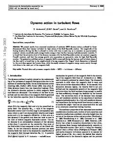
Randomness Representation in Turbulent Flows with ...

International Environmental Modelling and Software Society (iEMSs) 8th International Congress on Environmental Modelling and Software Toulouse, France, Sabine Sauvage, José-Miguel Sánchez-Pérez, Andrea Rizzoli (Eds.) http://www.iemss.org/society/index.php/iemss-2016-proceedings

Randomness Representation in Turbulent Flows with Bed Roughness Elements using the Spectrum of the Kolmogorov complexity a

b

c

a

D. T. Mihailović , G.Mimić , P. Gualtieri , I. Arsenić , and C. Gualtieri

c

a

Department of Field Crops and Vegetable, Faculty of Agriculture, University of Novi Sad, Dositej Obradovic Sq. 8, 21000 Novi Sad, Serbia; [email protected], [email protected] b Department of Physics, Faculty of Sciences, University of Novi Sad, Dositej Obradovic Sq. 4, 21000 Novi Sad, Serbia; [email protected] c Department of Civil, Architectural and Environmental Engineering, University of Naples Federico II, Via Claudio 21, 80125 Naples, Italy; [email protected], [email protected]

Abstract: One feature of turbulent flow in relation to randomness is quantified. Experimental data from a turbulent flow collected in a laboratory channel with bed roughness elements of different densities are used. An analysis based on a classical turbulence statistics is performed, using a simple empirical model for estimating the relative sizes of mixing lengths representing the typical scale of an eddy in the corresponding surface layer, to describe the turbulence in terms of irregular or random flow. Instead of such description a quantification of the turbulence flow using measures based on the spectrum of the Kolmogorov complexity (KC) is proposed. Keywords: turbulent flow, bed roughness elements, randomness, coherent structures, Kolmogorov complexity spectrum

1

INTRODUCTION

The influence of bed roughness elements on turbulent flow is a crucial topic in many different fields of the fluid mechanics (Jimenez, 2004; Poggi et al., 2004; Flack et al., 2005; Nezu and Sanjou, 2008; Cushman-Roisin et al., 2012). The aquatic plants in rivers have considerable effects on turbulence between the zones with and without vegetation (Nezu and Sanjou, 2008). In the presence of submerged bed roughness elements a roughness sublayer (RSL) is formed (Hussain, 1983; Raupach et al., 1996; Nepf, 2012). Within the RSL there exist three distinct zones (Figure 1a): (i) the deep zone (RS1); (ii) the RS2 zone is a superposition of attached eddies and Kelvin–Helmholtz waves produced around the inflection point on the mean velocity profile (Figure 1b), which develops between two coflowing streams having different velocities (Poggi et al., 2004). In this turbulent mixing region KelvinHelmholtz instability causes coherent turbulent structures that travel downstream in the environmental fluids (Hussain, 1983; Rogers and Moser, 1994; Raupach et al., 1996). The RS2 zone is a superposition of all three constituents; (iii) the RS3 zone is shifted rough wall boundary layer. For a long time, there was an interest in the fluids mechanics for a better understanding the physical processes involved in flow-roughness elements interaction, which includes interaction between zones described above, e.g., the turbulent boundary layer and outer laminar region, wall- and free-shear turbulent flows exhibiting coherent structure (Tsuji and Nakamura, 1994; Ichimiya and Nakamura, 2013). However, in the turbulent flow some problems remain unanswered because a more complete definition of turbulence was not yet proposed (Ichimiya and Nakamura, 2013). Namely, one of the fundamental properties in the definition of the turbulence is not clearly included and it is usually expressed verbally in terms of irregular or random fluid flows but without its quantification. An overview of such definitions is reported (Ichimiya and Nakamura, 2013). Only exception is Pope’s

D. T. Mihailović et al. / Randomness representation in turbulent flows with bed roughness elements …

definition of randomness related to turbulence (Pope, 2000), which cannot be used as a measure of the randomness in the sense of the Kolmogorov complexity (KC) (Li and Vitanyi, 1997), based on which Lempel and Ziv (1976) developed an algorithm for calculating the measure of the randomness (LZA). This algorithm is used for evaluation of the randomness in time series. The goal of this paper is to quantify randomness of turbulent flows that develop over bed roughness elements. The results from an experimental study carried out in a laboratory channel with variable bed slope at the University of Naples Federico II (Naples, Italy) are used. To estimate the turbulence randomness the KC complexity and complexity measures based on the KC are applied. In order to nearly quantify the randomness of the turbulence, an analysis based on classical turbulence statistics is performed, including a simple empirical model for the estimation of the relative sizes of mixing lengths representing the typical scale of an eddy in the corresponding part of the surface layer. Finally, the proposed measures of the randomness of turbulent flow in the surface layer are discussed.

Figure 1. (a) A schematic diagram of eddies structure over and within the bed roughness elements: (i) RS1 zone (z/k < 1; k is the height of the roughness element) where the flow field is primarily dominated by small eddies associated with the von Kármán streets; (ii) RS2 zone straddles the top portion of the bed roughness elements, and is dominated by a mixing layer and (iii) RS3 zone (z/k > 2) is the classical boundary-layer region dominated by eddies with length scales proportional to (z-d), where d is the displacement height. (b) The mean velocity profile within the bed roughness elements 2 u(z) =u(k) -β1e-β z +β2eβ z is obtained from the solution of the partial differential equation ∂u /∂z = 3

2

3

2

[(2Cdλdk )/(σsPs)]u where: u(k) is the velocity at the height k; β1,β2 are parameters depending on the morphological and aerodynamic characteristics of the bed roughness elements and β3 = 2 (2Cdλdk )/(σsPs)]; Cd - the drag coefficient; σs - the parameter of proportionality between the turbulent transport coefficient and velocity within the bed roughness elements; λd - the roughness density and Ps – the shelter factor.

2

MATERIALS AND METHODS

The experiments were performed in a laboratory channel with variable bed slope, which was 8 m long and 0.4 m wide (Figure 2a). Vegetation covered the bed of the channel and consisted of rigid cylinder rods of the same height and diameter (k=0.015 m, dc=0.004 m – Figure 2b), set in different aligned arrangements (rectangles or squares), with three different densities λd (Table 1). Vegetation density was evaluated as the total roughness elements frontal area per unit area. The vegetation was always fully submerged with submergence hu/k, of about 4, where hu is the uniform flow depth. The experimental conditions are listed in Table 1, where: ub is the bulk velocity or depth-averaged velocity, u* is the shear velocity and uk is the velocity at the top of the bed roughness elements. Instantaneous values of streamwise velocities were recorded in uniform flow in a vertical cross section located at the mid-length of a square or rectangular array. The velocity measurements were carried out in about twenty-five vertical locations using a laser Doppler velocimeter (LDV) equipped with a frequency shifter and a frequency tracker. The sampling frequency for the LDA measurements was 2000 Hz and, in order to obtain a sufficient number of strong bursting events, the acquisition time in each


measurement point was equal to 135 s, so the sampling data of N=270000 of instantaneous velocity were collected and analyzed for turbulent statistics. The sampling frequency and the sampling time were selected to accurately represent the investigated flow and to result in data files supported by the software package used for computation. For commercial LDA systems, processor information is converted to velocity through software with equation V x = λ fD, where the uncertainty in the wavelength of the laser is negligible. For modern signal processors, the uncertainty in the measurement of the Doppler frequency can be assumed negligible. In (Nezu 2001) the most accurate measurement device was LDA and the accuracy of a PIV was validated by comparing PIV data with LDA data. For each measurement point, the analog signal from the processor was carefully checked by means of an oscilloscope to verify the Doppler signal quality, as in (Poggi et al. 2002). The turbulent data were post-processed using the LabView software to derive the distribution of time-averaged velocity, and standard deviation related to turbulence intensity.

(a)

(b)

Figure 2. (a) Channel and (b) vegetated bed.

Test D1 D2 D3

d

Q

hu

(m m )

Slope o ()

(l s )

(cm)

0.024 0.048 0.096

0.03 0.02 0.03

33 22 22

6.35 6.44 6.29

2

-3

-1

Cylinders per unit area 400 800 1600

ub

uk

u* -1

-1

-1

(m s )

(m s )

(m s )

1.128 0.735 0.715

0.119 0.098 0.119

1.192 0.763 0.726

Table 1. Experimental conditions. The Kolmogorov complexity K(x) of an object x is the length, in bits, of the smallest program that when run on an Universal Turing Machine (U) prints object x, which is maximized for random strings (Lempel and Ziv, 1976). A complete description of the KC can be found in Feldman and Crutchfeld (1998). The complexity K(x) is not a computable function of x. However, a suitable approximation considered as the size of the ultimate compressed version of x, and a lower bound for what a real compressor can be achieved (Cerra and Datcu, 2011). Therefore, we point out that all the measures used in this paper are measures derived from the computable approximation of KC. The KC complexity of a time series {xi}, i = 1,2,3,…,N by the LZA algorithm includes the following steps. (1) Encoding the time series by constructing a sequence S of the characters 0 and 1 written as {s(i)}, i = 1,2,3,…,N, according to the rule {s(i)} = {0, xi < x*; 1, xi ≥ x*}. Here for x* the mean value of the time series is used as threshold (Zhang et al., 2001). (2) Calculating the complexity counter c(N). The c(N) is defined as the minimum number of distinct patterns contained in a given character sequence. The complexity counter c(N) is a function of the length of the sequence N. The value of c(N) is approaching an ultimate value b(N) as N approaching infinite, i.e. c(N) = O(b(N)) and b(N) = N/log2N. (3) Calculating the normalized information measure Ck(N), which is defined as Ck = c(N) / b(N) = c(N) log2N / N. For a nonlinear time series, Ck(N) varies between 0 and 1. Notably, when a value of the KC is close to zero then it is associated with a simple deterministic process like a periodic motion, whereas a value close to one is associated with a stochastic process. The KC complexity as a measure does not make a distinction between time series with different amplitudes and similar random components. Thus, to better quantify the randomness of the turbulent flows over bed roughness elements analyzed in this paper, two measures based on the Kolmogorov complexity are used: (i) the Kolmogorov complexity spectrum and (ii) the Kolmogorov complexity spectrum highest value (Mihailović et al., 2015). Here, we shortly describe those following Mihailović et al. (2015). The time series {xi}, i = 1,2,3,…,N is normalized performing the transformation xi = (XiXmin)/(Xmax-Xmin), where Xi is a time series obtained by the measurements where: Xmax = max(Xi) and


Xmin=min(Xi). It means that all elements in time series {xi} are placed in the interval [0, 1]. The Kolmogorov complexity spectrum of time series {xi} is the sequence {ci}, i=1,2,3,…,N obtained by the LZA algorithm which is applied N times on time series, where thresholds {xt,i} are all elements in {xi}. To be precise, the elements of the original time series are transformed into a set of 0-1 sequences k (k) {Si }, i=1,2,3,…,N; k=1,2,3,…,N defined by comparison with a threshold {xt,k} as {Si } = {0, xi < xt,k; 1, (k) xi ≥ xt,k}. Applying the LZA algorithm on each element of the series {Si } the KC complexity spectrum {ci}, i = 1,2,3,…N is obtained. This spectrum allows us to investigate the range of amplitudes in a time series representing a process, for which it has highest complexity, i.e. highly enhanced stochastic C C components. The highest value K max in this series, i.e. K max = max{ci}, is the Kolmogorov complexity spectrum highest value (KCM).

3

RESULTS AND DISCUSSION

Figures 3a-3c show the distributions of the streamwise local mean velocity U (u = U + u', where u and u' are instantaneous streamwise measured velocity and velocity fluctuation, respectively) at several relative heights z/k within and above the bed roughness elements for three different densities (D1, D2 and D3). These figures show that vertical velocity profiles over bed roughness elements of different densities do not follow standard logarithmic profile. For z/k =1 and densities D1 and D3, the inflection points and the shape of velocity profiles follow the theoretical curve in Figure 1b. According to the vertical velocity distribution, the flow could be separated into two zones: (i) a lower zone within the bed roughness elements (z/k < 1) and (ii) an upper zone (z/k > 1). However, these comments can be just partly addressed to the velocity profile for the density D2 (Figure 3b). Let us point out that the most essential difference among velocity profiles relative to different densities is the magnitude of the inflection in the profile where z/k =1, which is a necessary condition for the occurrence of Kelvin– Helmholtz instabilities. However, according to Poggi et al. (2004) its magnitude assigns a framework of the relative importance of that mechanism on the whole turbulence structure. The turbulence statistics applied on measured values of velocity quantify how the flow within and just above the bed roughness elements behaves as a perturbed mixing layer. Here, we express the N

turbulence intensity as u =

u

2 i

/ N normalized by the friction velocity u*, i.e. σu=ū/u*. The number

i=1

of the samples was N=270000. 3

3

3

D1

D3

D2

2

2

2

z/k

z/k

z/k

1

1

1

(a) 0 0.5

1.0

u(z)/uk

1.5

(c)

(b) 0 0.5

1.0

u(z)/uk

1.5

0 0.5

1.0

1.5

u(z)/uk

Figure 3. Time-averaged mean vertical velocity profiles for all the densities normalized by the velocity at the roughness elements top (uk). Figure 4a depicts the measured profiles of σu for all three densities D1, D2 and D3. From this figure it is clear that increasing λd, turbulence intensity σu is remarkably damped for z/k < 1. It is seen, that σu changes from 1.69 (D1), for sparse roughness elements, which is typical for rough-wall layers, to about 1.49 (D3) for dense roughness elements, which is typical for mixing layers. Those values are close to ones reported by Jimenez (2004). Further inspection of this figure shows that for all densities σu increases from the bed to the top of the roughness elements (z/k < 1). Above this σu weakly decreases in RS2 zone and towards the free surface (i.e., in the RS3 zone). These measures of the traditional turbulence statistics provide an insight in the structure of turbulence within the bed


roughness elements and of the coherent motions near their top. To explain the behavior of σu we calculate empirically the three basic length scales lv, lml and lbl for RS1, RS2 and RS3 zones, respectively partly following parameterization by Poggi et al. (2004). In RS1 zone, where the flow field is primarily dominated by small vortices associated with the von Kármán streets, the mixing length is evaluated as lv = dr/0.21. The mixing length lml in the RS2 zone, i.e. the mixing layer, is parameterized as lml = ūk/(dū/dz)z=k. Finally, the RS3 zone is a classical boundary-layer dominated by eddies with length scales lbl = κ(z-d), where κ is the von Kármán constant. The relative mixing lengths lv, lml and lbl normalized by k, calculated for all the densities, with zero plane displacement d equal to 2/3 k, are depicted in Figure 4b. The calculated values of the relative sizes of mixing lengths are the following: (1) lv/k =0.85 and lbl/k = 0.82 in the RS1 and RS3 zones, respectively for all the densities and (2) lml/k = 2.20 (D2), 1.47 (D1, D3) in the RS2 zone, respectively. Here, the relative sizes of mixing lengths lv/k, lml/k, and lbl/k represent the typical scale of an eddy in the corresponding layer. Eddies in all three zones are visualized in Figure 4b. In RS1 zone von Kármán eddies are smaller with sizes proportional to dr and independent of λd and local velocity (Poggi et al., 2004). In RS2 zone eddies are larger, organized in a coherent structure, carrying the highest amount of energy, while in RS3 zone they are again of smaller size. This simple consideration empirically explains the behavior of σu in Figure 4a. However, we still have no available measure of randomness, which is a crucial property of the turbulence as we stressed in the introduction. 3 D1 D2 D3

2

z/k 1

(a) 0 0

1

Turbulence intensity,

2 u

Figure 4. Turbulence intensity ū normalized by u* (a) and mixing lengths lv, lml and lbl normalized by k (b) against relative flow depth ratio of vertical distance from bed z to bed roughness elements height k for all the densities. The relative sizes of mixing lengths lv/k, lml/k, and lbl/k which are calculated representing the typical scale of an eddy in the corresponding layer. When stable laminar flows evolve toward the turbulence, they become high-order and complex, exhibiting irregular-like motions with organized dissipative arrangements. In order to precisely specify their fields (velocity and displacement) more parameters are required than for description of laminar flows, i.e. topological measures that quantify the order or disorder of the flow. One such measure is the Shannon entropy, which has been already used in analyses of geophysical fluids (Wijesekera and Dillion, 1997; Wesson et al., 2003). The Shannon entropy SH is defined as SH = -Σ pi ln pi where pi is a discrete probability distribution satisfying the following conditions: pi ≥ 0; Σ pi = 1 and piUjU... = pi+pj+… (Shannon, 1948). In our calculations pi is defined as a probability that velocity amplitude falls within interval ui+du, where du is obtained dividing entire interval of velocity amplitudes into N intervals. Figure 5a shows that the SH is the highest in the mixing layer (1 < z/k < 2) where the turbulence intensity σu is the highest. However, it decreases towards the free surface. This behavior of the SH coincide with conclusion by Wijesekera and Dillion (1997). A decrease of the SH going to the rough bed can be addressed to the occurrence of smaller eddies carrying smaller amount of the energy.


3

3 D1

D1

D2

D2

D3

D3

2

2

z/k

z/k 1

1

(a) 0 0.40 0.45 0.50 0.55 0.60

Shannon entropy, SH

(b) 0 0.2

0.3

0.4

0.5

0.6

Kolmogorov complexity, KC

Figure 5. Shannon entropy (SH) (a) and Kolmogorov complexity (KC) (b) versus relative flow depth ratio of vertical distance from bed z to bed roughness elements height k for all the densities. To avoid confusion in the following discussion we will make some comments. Namely, the term complexity in physical systems has connotation of an explicit measure of the probability of the state of the system. It is a mathematical measure which should not be equalized with entropy in statistical mechanics (Mihailović et al., 2015). Thus, the Shannon’s entropy refers to dissimilarities between amplitudes in a time series, while the Kolmogorov complexity refers to the apparent sequence disorder of some amplitudes in a time series. This complexity that we intuitively understand as a measure ranged between uniformity and total randomness (Figure 3 in Mihailović et al., 2015) is of interest in this paper. Comparing figures 5a and 5b, they seem overall to have quite symmetrical trends. In figure 5a the randomness weakly increases in RS1 zone; it has a constant value in RS2 zone and then decreases in the RS3 zone. This trend is more clear for sparse bed roughness elements (D1) but, anyway, the density of the bed roughness elements seems to affect randomness, in fact lower randomness corresponds to sparse density (D1). Figure 5b shows that the value of the KC complexity decrease with height from the rough-wall to the mixing layer (1 < z/k < 2). This can be explained by the fact that in the RS1 zone flow is dominated by smaller eddies (see Figure 4b) contributing to the higher randomness which becomes lower in the mixing layer having a constant value in this zone. This is because eddies in this zone are larger and coherently organized, without possibility to introduce more randomness in the flow. Above the mixing layer the KC slightly increases since eddies become smaller providing conditions for higher complexity in flow. Using the LZC algorithm and definitions about the complexity measures based on the Kolmogorov complexity, for all the densities and selected relative flow depth ratio z/k, Kolmogorov spectra have been calculated and depicted in Figure 6. These figures show that the KCM values (when the randomness is the highest) are very close to the KC at the corresponding relative heights (Figure 5b). Moreover, as the density increases, Kolmogorov spectra in the mixing layer, where complexity is constant, tend to be close each other. However, the Kolmogorov spectrum provides us additional information. Namely, the area below this spectrum (overall complexity in Mihailović et al., 2015, which is not considered in this paperr) gives integral information about complexity for the whole spectrum of complexities, i.e., it comprises both (i) dissimilarities between amplitudes (SH) and (ii) disorder of some amplitudes (KC). Thus, the Kolmogorov based complexity measures allow to quantify the degree of turbulence in relation to randomness rather than it is expressed verbally in terms of irregular or random.

Kolmogorov complexity


1.0 0.9 D1 0.8 0.7 0.6 0.5 0.4 0.3 0.2 (a) 0.1 0.0 0.0 0.1 0.2 0.3 0.4 0.5 0.6 0.7 0.8

z/k 0.067 0.4 1 1.8 2.667

0.9 1.0


Normalized amplitude 1.0 0.9 D2 0.8 0.7 0.6 0.5 0.4 0.3 0.2 (b) 0.1 0.0 0.0 0.1 0.2 0.3 0.4 0.5 0.6 0.7 0.8

z/k 0.067 0.4 1 1.8 2.667

0.9 1.0


Normalized amplitude 1.0 0.9 D3 0.8 0.7 0.6 0.5 0.4 0.3 0.2 (c) 0.1 0.0 0.0 0.1 0.2 0.3 0.4 0.5 0.6 0.7 0.8

z/k 0.067 0.4 1 1.8 2.667

0.9 1.0

Normalized amplitude

Figure 6. Kolmogorov spectra for all the densities and selected relative flow depth ratio of vertical distance from bed z to bed roughness elements height k.

4

CONCLUSIONS

In this paper a methodology to quantify the randomness in turbulent flows with bed roughness elements using experimental data collected in a laboratory channel with variable bed slope and three different bed roughness element densities is described. An analysis based on the KC, i.e., spectrum of Kolmogorov complexity and KCM was proposed. First, the turbulence was analyzed by the classical turbulence statistics, for all the densities, through vertical profiles of streamwise velocity, turbulence intensity and Shannon entropy (SH) in addition, including the use of a simple empirical model for the estimation of the relative sizes of mixing lengths in surface layer, to describe the turbulence in terms of irregular or random flow. Then, the complexity metrics were applied to all the densities. Finally, it was showed that the Kolmogorov complexity based measures allow to quantify the degree of turbulence in relation to randomness rather than it is expressed descriptively in terms of irregular or random.


ACKNOWLEDGMENTS This paper was realized as a part of the project No. 43007 financed by the Ministry of Education and Science of the Republic of Serbia for the period 2011-2015. The Italian authors acknowledge even the support by the MIUR PRIN 2010-2011 research project “HYDROCAR”. The authors are grateful to Professor Borivoj Rajković for his valuable comments.

REFERENCES Cerra, D., Datcu, M., 2011. Algorithmic relative complexity. Entropy 13, 902-914. Cushman-Roisin, B., Gualtieri, C., Mihailović, D.T., 2012. Environmental Fluid Mechanics: Current issues and future outlook. In: Gualtieri, C., Mihailović, D.T. (Eds), Fluid Mechanics of Environmental nd Interfaces, 2 ed., CRC Press/Balkema, Leiden, Holland, 3-17. Feldman, D.P., Crutchfeld, J. P., 1998. Measures of statistical complexity: Why? Phys. Lett. A 238, 244-252. Flack, K. A., Schultz, M. P. Shapiro, T., 2005. Experimental support for Townsend’s Reynolds number similarity hypothesis on rough walls. Phys. Fluids 17, 035102. Hussain, A. K. M. F., 1983. Coherent Structures - Reality and Myth. Phys. Fluids 26, 2816-2850. Ichimiya, M., Nakamura, I., 2013. Randomness representation in turbulent flows with Kolmogorov complexity (In laminar-turbulent transition due to periodic injection in an inlet boundary layer in a circular pipe). J. Fluid Sci. Techn. 8, 407-422. Jimenez, J., 2004. Turbulent flows over rough walls. Annu. Rev. Fluid Mech. 36, 173–196. Lempel, A., Ziv, J., 1976. On a complexity of finit sequence. IEEE Trans. Inform. Theory 22, 75–81. nd Li, M., Vitanyi, P., 1997. An Introduction to Kolmogorov Complexity and its Applications, 2 ed., Springer Verlag, Berlin, Germany. Mihailović, D. T., Mimić, G., Nikolić-Djorić, E., Arsenić, I., 2015. Novel measures based on the Kolmogorov complexity for use in complex system behavior studies and time series analysis. Open Phys. 13, 1–14. Nepf, H. M., 2012. Flow and transport in regions with aquatic vegetation. Annu. Rev. Fluid Mech. 44, 123–142. Nezu, I., Onitsuka, K., 2001. Turbulent structure in partly vegetated open channel flows with LDA and PIV measurements. Journal of Hydraulic Research 39, 629e642. Nezu, I., Sanjou, M., 2008. Turbulence structure and coherent motion in vegetated canopy openchannel flows. J. Hydro-Environ. Res. 2, 62-90. Poggi, D., Porporato, A., and Ridolfi, L., 2002. An Experimental Contribution to Near-Wall Measurements by Means of a Special Laser Doppler Anemometry Technique. Exp. Fluids 32, 366– 375. Poggi, D., Porporato, A., Ridolfi, L., Albertson, J.D., Katul, G. G., 2004. The effect of vegetation density on canopy sub-layer turbulence. Bound-Lay Meteorol. 111, 565– 587. Pope, S. B., 2000. Turbulent Flows, Cambridge University Press, Cambridge, UK. Raupach, M. R., Finnigan, J. J., Brunet, Y., 1996. Coherent eddies and turbulence in vegetation canopies: the mixing-layer analogy. Bound-Lay. Meteorol. 78, 351-382. Rogers M. M., Moser, R. D., 1994. Direct simulation of a self-similar turbulent mixing layer. Phys. Fluids 6, 903-923. Tsuji, Y., Nakamura, I., 1994. The fractal aspect of an isovelocity set and its relationship to bursting phenomena in the turbulent boundary layer. Phys. Fluids 6(10), 3429-3441. Shannon, C. E., 1948. A mathematical theory of communication. Bell Syst. Tech. J. 27, 379–623. Wesson, H. K., Katul, G. G., Siqueira, M., 2003. Quantifying organization of atmospheric turbulent eddy motion using nonlinear time series analysis. Bound-Lay. Meteorol. 106, 507–525. Wijesekera, H. W., Dillion, T. M., 1997. Shannon entropy as an indicator of age for turbulent overturns in the ocean thermoclines. J. Geophys. Res. 102, 3279–3291. Zhang, X. S., Roy, R. J., Jensen, E. W., 2001. EEG complexity as a measure of depth of anesthesia for patients. IEEE Trans. Biomed. Eng. 48, 1424-1433.