Range-Based Density Control for Wireless Sensor Networks

Range-Based Density Control for Wireless Sensor Networks Yang-Min Cheng Li-Hsing Yen Dept. Computer Science & Information Engineering Chung Hua University Hsinchu, Taiwan 300, R.O.C. {cs88625, lhyen}@chu.edu.tw

Abstract Density control in a wireless sensor network refers to the process of deciding which node is eligible to sleep (enter power-saving mode) after random deployment to conserve energy while retaining network coverage. Most existing approaches toward this problem require sensor’s location information, which may be impractical considering costly locating overheads. This paper proposes a new density control protocol that needs sensor-to-sensor distance but no location information. It attempts to approach an optimal sensor selection pattern that demands the least number of working (awake) sensors. Simulation results indicate that the proposed protocol is comparable to its location-based counterpart in terms of coverage quality and the reduction of working sensors.

1. Introduction Rapid progress in wireless communications and microsensing MEMS technology has enabled the deployment of wireless sensor networks. A wireless sensor network consists of a large number of sensor nodes deployed in a region of interest. Each sensor node is capable of collecting, storing, and processing environmental information, and communicating with other sensors. The positions of sensor nodes need not be engineered or predetermined [1] for the reason of the enormous number of sensors involved [3] or the need to deploy sensors in inaccessible terrains [1]. Due to technical limitations, each sensor node can detect only events that occur within some range from it. A piece of area in the deployment region is said to be covered if every point in this area is within the sensory range of some sensor. The area that are collectively covered by the set of all sensors is referred to as network coverage. As sensor nodes are usually powered by batteries, powerconserving techniques are essential to prolong their opera-

tion lifetimes. In this paper, we are considering powering off redundant sensors temporarily after random deployment to conserve energy while retaining network coverage. Density control is a process deciding which node is eligible to sleep (entering power-saving mode), while node scheduling arranges the sleep time. Existing approaches toward density control are mostly location-based [8, 7, 6, 12, 4, 9], meaning that these approaches require location information of sensors. Locationbased density control algorithms can ensure 100% network coverage. However, the requirement of location information may not be practical if energy-hungry GPS (Global Positioning System) device is assumed for this purpose. There are other approaches that control density based on the count of working neighbors [10], the current node density [6], or the network coverage expected [11]. These approaches demand no locating devices and are thus more suitable for small-size sensors. However, it is intrinsic that 100% network coverage cannot be guaranteed. This paper proposes a new density control protocol that needs no location information. It attempts to approach an optimal sensor selection pattern that demands the least number of working (awake) sensors. Our approach needs sensor-to-sensor distance information, which can be acquired by some range measurement technique. We conducted extended simulations for performance comparisons among our protocol and other counterparts. The results indicate that our protocol performs nearly well as a locationbased scheme can do in terms of coverage quality and the reduction of working sensors. The rest of this paper is organized as follows. The next section reviews existing density control protocols and Section 3 details our work. Experimental results are presented in Section 4. The last section concludes this paper.

2. Related Work and Motivation PEAS [10] is a node density control protocol that demands no location information. In PEAS, all nodes are

initially sleeping. These nodes awake asynchronously and broadcast a probe message. Any working node receiving the message should reply. If an awakening node receives a reply to the probe message, it enters sleep mode again. Otherwise, it becomes a working node for the rest of its operation life. The performance of PEAS heavily depends on probing range, the transmission range of the probe message. A small probe range usually leads to high coverage ratio but also a large population of working node. There are also stochastic approaches that alter node density without location information. In the scheme proposed in [6], all nodes randomly and independently alternate between working and sleep modes on a time-slot basis. Given the probability that a sensor is in working mode, the authors have analyzed the probability of a point being uncovered. In [11], the time periods of working and sleep modes are exponentially distributed random variables. Though the method is stochastic in nature, it is deterministic to set the means of these two distributions for a specific expected network coverage. Most existing density control protocols require location information. C˘arbunar et al. [4] transform the problem of detecting redundant sensors to that of computing Voronoi diagrams. Node location information is required in their scheme to compute the Voronoi diagram corresponding to the current node deployment. Xing et al. [9] also exploit Voronoi diagram to ensure k-coverage, which refers to the condition that every point in the deployment region is covered by at least k sensor nodes. They have shown that kcoverage is ensured if every critical point (where two sensor’s coverage areas intersect or a sensor’s coverage area and border line intersect) is covered by at least k sensors. The protocol they proposed needs location information of every sensor as well. A coverage-preserving density control scheme presented in [8] demands that each sensor advertises its location information and listens to advertisements from neighbors. After calculating its coverage and its neighbors’, a node can determine if it is eligible to turn off its sensory circuitry without reducing overall network coverage. To avoid potential “coverage hole” due to simultaneous turning off, a back-off protocol is proposed that requires each off-duty eligible sensor to listen to other sensor’s status advertisement and, if necessary, announce its own after a random back-off time period expires. The behaviors of some other schemes [7, 6, 12] are similar to [8] in that they all require the exchanges of location information and eligibility status. Among them, OGDC [12] aims to arrange a particular deployment pattern of working sensors. It has been shown [12] that, to minimize the population of working sensors while preserving network coverage, the locations of any three neighbor sensors should form an equilateral triangle with side length √ 3rs , where rs is the sensory range. Extending this argu-

D

F

B

A

S

E

C

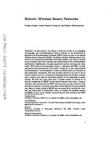
Figure 1. Optimal deployment pattern that demands the least number of working sensors to cover entire region

ment, the optimal deployment pattern that requires the least number of working sensors should be that shown in Fig. 1. Each working sensor S is surrounded by six working neighbors (co-workers)√ that from a regular hexagon centered at S with side length 3rs . Provided that the node density is sufficiently high, it is feasible to seek such a pattern among all deployed sensors. Network connectedness is another issue that should be addressed in density control. It has been proven [12, 9] that given 100% coverage ratio, rt ≥ 2rs suffices to ensure network connectedness, where rt is the transmission range of every sensor. Many protocols [12, 9] therefore focus on maintaining full coverage and simply set rt = 2rs to ensure network connectedness at the same time. Our approach assumes the availability of a ranging technology that estimates the distance between pair-wise neighbors. Several ranging techniques have been proposed for wireless sensor networks. One possible way is to establish a mathematical or empirical model that describes radio signal’s path loss attenuation with distance [2]. A received signal strength indication (RSSI) can thereby be translated into a distance estimate. Another trend of ranging technologies turns signal propagation time into distance information. If the sender and the receiver of a radio signal are precisely time-synchronized, the distance in-between can be derived from the time of arrival (ToA). If two signals (one is RF and the other is acoustic signal, for example) are transmitted simultaneously, the time difference of the arrivals (TDoA) can be used for ranging [5]. Signal propagation problems such as environmental interference and multi-path fading introduce estimation errors to almost all existing ranging technologies. The degree of errors is environment-dependent. In harsh networking environments, the errors can be so high that makes ranging techniques ineffective. Nevertheless, we assume a perfect ranging scheme behind our work. The motivation of this research is merely to see how well density control can be done

Sleep

Table 1. Parameter/Timer setting Parameter/Timer Value p0 1/n √ rt 3rs Ts [0, 0.01] Tp [0, 0.1] To 2 Te 0.05 Td 0.25 Tc 5 D1 rt /2 D2 rs Note: An interval value means a value randomly generated within the interval. with range but location information. The results therefore only stand for those of a best-case study.

3. Proposed Scheme The basic idea behind our approach is that the deployment pattern shown in Fig. 1 can be approached without exact location information. If the √ transmission range of each sensor in Fig. 1 is uniformly 3rs , S’s co-workers are exactly S’s neighbors that have the maximum transmission distance to S. S can first search for one such co-worker, say, A, then repeatedly looks for nodes that are both the coworkers of S and an already-found co-worker. If the second co-worker found is B (C), the third co-worker will be C or D (B or E). If the third co-worker is B or C, the fourth co-worker will be D or E. In this way, all six co-workers, if exist, can be found without knowing their exact locations.

3.1. Protocol Description Our protocol uses three control messages: C O - WORKER R EQUEST, C O - WORKER R ESPONSE, and R ECRUITMENT D ONE. Table 1 lists settings of some parameters and timers used by our protocol. Every sensor locally maintains two lists: neighbor list and co-worker list. The former keeps the ID (identification) and distance of each neighbor. The latter records the IDs of known co-workers. Every C O - WORKER R EQUEST sent by a sensor is attached with the sender’s ID and its co-worker list. Figure 2 shows the state transition diagram of the proposed protocol. All nodes are initially in Role-deciding state, where each node tests if it can become a starting node, a node that initiates co-worker recruitment. The test is pure stochastic; a node can be a starting node with initial probability p0 , where p0 is a variable inversely proportional to

Sleep eligible

Sleep eligible

Role-deciding

Co-worker Response scheduled

Test succeeded & Ts expired Starting Node

To expired

Become a co-worker Waiting

Co-worker

Tc expired To expired Working

Figure 2. State transition diagram of the proposed protocol

the node density of the network. If the test fails, the node conducts the test again in the following second. The probability of success exponentially increases with time: it is min{2i−1 p0 , 1} in the ith second. The process repeats until the test succeeds or the node hears C O - WORKER R E QUEST from one of its neighbors. The latter case indicates that some neighbor has successfully become a starting node. The node ceasing the test process then executes the procedure shown in Fig. 3 to decide whether it is eligible to sleep or should be a co-worker of its neighbor.

if the distance between S and R is less than D1 then enter sleep mode directly; skip all the following steps if R is listed in the attached co-worker list then wait Tp seconds broadcast Co-worker Request and set timer To go to Co-Worker state else // R has not yet replied to S determine if R should reply by the rule shown in Table 2 if R need not reply then enter sleep mode directly if S is not in R’s neighbor list then add S into R’s neighbor list for each node i that is in the attached co-worker list do add i to R’s co-worker list if i is R’s neighbor set Tr according to Table 2 go to Waiting state end if

Figure 3. The procedure for node R to process Co-worker Request received from S

When the test succeeds, the node waits Ts seconds before broadcasting C O - WORKER R EQUEST. The value of Ts is randomly chosen to avoid possible transmission colli-

0.7 0.6

Note: L and N are the sets of S’s co-workers and R’s neighbors, respectively. sions that may occur when multiple nearby sensors decide to send C O - WORKER R EQUEST at the same time. If no C O WORKER R EQUEST is heard during that interval, the node broadcasts C O - WORKER R EQUEST, sets timer To , and then enters Starting Node state. If the node hears another C O WORKER R EQUEST before it issues its own, the procedure in Fig. 3 is executed. The procedure in Fig. 3 decides whether a node receiving C O - WORKER R EQUEST is eligible to sleep or should be a co-worker. Suppose that R receives C O - WORKER R E QUEST from S. If R is close to S (i.e., R’s distance to S is less than D1 ), R will enter sleep mode directly as it does not contribute substantial coverage to S. Otherwise, the “else” part of the outer if-statement will be executed, as R has not yet responded to any C O - WORKER R EQUEST and thus cannot be a co-worker of anyone. The code segment there determines whether R need reply to S’s request and, if it need, how long it should wait before sending the reply. Table 2 details the decision rule. If more than two of R’s neighbors are already S’s co-workers, R can sleep for its expected-low coverage contribution. Otherwise, the value of the reply delay timer Tr is chosen to let the most appropriate node (the one that is closest to the intended location) reply first. The setup of Tr involves calculating the value of dtime. For any C O - WORKER R EQUEST sent from S to R, let L and N be the sets of nodes that are the listed co-workers of S and the neighbors of R, respectively. dtime in Table 2 is defined as X dtime = D(S, R) + D(R, j). (1) j∈L∩N

Function D(i, j) is defined as µ µ ¶¶ di,j D(i, j) = 1 − exp −1 , rt where di,j is the distance between nodes i and j. See Fig. 4. After Tr is set, R enters Waiting state, in which the C O WORKER R ESPONSE is scheduled to be sent to S when

0.5

D(i,j)

Table 2. The rule of replying Co-worker Response Condition |L| |L ∩ N | Reply? Tr 0 0 Yes dtime 0 Yes dtime+Td ≥1 1 or 2 Yes dtime >2 No −

0.4 0.3 0.2 0.1 0 0

0.2

0.4

0.6

0.8

1

d /r i,j

t

Figure 4. The value of D(i, j) versus the ratio of di,j to rt

Tr expires. R cancels the scheduled sending (by resetting Tr ), however, if it overhears a C O - WORKER R ESPONSE addressed to S at any time before Tr expires. R does this because the sender of the C O - WORKER R ESPONSE is more qualified to be S’s co-worker than R. The overheard C O WORKER R ESPONSE updates R’s neighbor list to include the sender’s ID. If a new C O - WORKER R EQUEST is received before Tr expires, the scheduled sending is canceled as well and the incoming message is processed by the same procedure shown in Fig. 3. The action of aborting the scheduled response on the receipt of a new request deserves a further note. The sender of the new request can be an independent starting node or a co-worker of the one that initiates the first request. We may devise a thoughtful yet complicated scheme to resolve the race condition between the old and the new requests. However, we found through simulations that doing so does not improve the results significantly. Therefore, we choose to ignore the old request for the sake of simplicity and the likelihood of saving power. This approach can save power as the early sender, expected to be a co-worker firstly, may be proved sleep-eligible later by the second or subsequent requests. After sending C O - WORKER R ESPONSE, R sets timer Tc and stays in Waiting state. Subsequent C O - WORKER R E QUEST received before Tc expires, if any, is processed by the same procedure (Fig. 3), where the “if” part of the second if-statement is executed if the co-worker list attached with the received request contains this node’s ID. In that case, this node has been recruited by some starting node. The node then broadcasts its own C O - WORKER R EQUEST and enters Co-Worker state. If no further message is received before Tc expires, the node enters working mode directly. If a R ECRUITMENT D ONE is received and its distance to the sender is less than D2 , the node enters sleep mode directly. Before node S enters Starting Node or Co-worker state, it must have broadcasted a C O - WORKER R EQUEST mes-

On receiving Co-worker Response from node R add R’s ID and distance to S into S’s neighbor list if the message is addressed to S and R is not S’s co-worker then add R’s ID to S’s co-worker list if first received then reset timer To set timer Te first received = false end if end if expired Te then broadcast Co-worker Request with the updated co-worker list set timer To first received = true end expired expired To then broadcast R ECRUITMENT D ONE end expired

Figure 5. The procedure for node S to process Co-worker Response replied by R. first received is initially true.

sage and set timer To . In either state, if the corresponding C O - WORKER R ESPONSE is not received before To expires, S simply broadcasts R ECRUITMENT D ONE and then enters working mode. If a C O - WORKER R ESPONSE from node R is received or overheard, S puts R into its neighbor list. If R is not yet S’s co-worker and this message is addressed to S (i.e., not a overheard message), S adds R into its co-worker list, resets To , waits some time for additional responses (if any), and then broadcasts a new C O - WORKER R EQUEST with the updated co-worker list. This gives S another call for additional co-workers and also instructs all its new coworkers to start their own recruitment. The detailed procedure for handling C O - WORKER R ESPONSE is shown in Fig. 5.

3.2. Discussion We shall now analyze the range of dtime and then clarify the design philosophy behind the decision rule shown in Table 2. Let di,j be the distance between nodes i and j. For a node R receiving C O - WORKER R EQUEST from node S, we have dS,R ≥ 0.5rt since otherwise R will enter sleep mode directly. It follows that 0 ≤ D(S, R) ≤ 1 − e−0.5 . For all other nodes j ∈ L ∩ N , where L and N are the sets of S’s co-workers and R’s neighbors, respectively, we have 0 ≤ D(R, j) ≤ 1 − e−1 since 0 ≤ dR,j ≤ rt . Accordingly,

B

C

S

A

C

S

(a)

A

(b)

Figure 6. S is a staring node and A is a recruited co-worker. Solid and dotted lines correspond to sensory and communication ranges, respectively.

the range of dtime is  [0, 1 − e−0.5 ]    [Td , 1 − e−0.5 + Td ] [0, 2 − e−0.5 − e−1 ]    [0, 3 − e−0.5 − 2e−1 ]

if |L| = 0, if |L| > 0 and |L ∩ N | = 0, if |L| > 0 and |L ∩ N | = 1, if |L| > 0 and |L ∩ N | = 2.

The objective of the decision rule in Table 2 is to pick up sensors that nearly form an equilateral triangle to be working nodes. First consider the scenario in Fig. 6(a), where S is a staring node and A is a co-worker that has responded to S’s request. Suppose now S broadcasts the second C O WORKER R EQUEST. Though it appears that C contributes a larger coverage area than B does, S should recruit B rather than C in this case as nodes S, A, and B nearly form an equilateral triangle. C should be recruited later. By Table 2 and (1), B will respond to S after D(S, B) + D(B, A) seconds (as |L| = 1 and |L ∩ N | = 1) while C will do so after D(S, C) + Td seconds (as |L| = 1 and |L ∩ N | = 0). Observe that D(S, B) ' D(S, C), so B’s response will be sent earlier than C’s if dB,A > 1 + ln(1 − Td ). rt

(2)

With the default value of Td (0.25 in Table 1), (2) implies that B will respond earlier than C (and hence causes a cancellation of C’s response) if dB,A > 0.71rt . Therefore, B rather than C will be the next recruited co-worker. Nevertheless, C still has the chance to respond to the second C O WORKER R EQUEST. But this happens only when B’s response message is garbled due to transmission errors, similar to the case of C in Fig. 6(b). Next consider the scenario in Fig. 7, where S is a staring node and A and B are recruited co-workers. Suppose now S broadcasts the third C O - WORKER R EQUEST. In Fig. 7(a), C should respond earlier than D because S, B, and C nearly form an equilateral triangle. (C also contributes a larger coverage area than D does.)

55

160 Ours

Ours

D

B D

C

A

S

C

A

S

OGDC PEAS (probing range = 8)

45

PEAS (probing range = 9) PEAS (probing range = 10)

40

OGDC

140

Number of working nodes

B

Number of working nodes

50

35 30 25

PEAS (probing range = 8) PEAS (probing range = 9) 120

PEAS (probing range = 10)

100

80

60

20 15

40 200

400

600

800

1000

200

(a)

(a)

(b)

Figure 7. S is a staring node and A and B are recruited co-workers. Solid and dotted lines correspond to sensory and communication ranges, respectively.

Probing range (for PEAS) Data transmission rate

By our design, C will respond to S after D(S, C) + D(C, B) ' 0 seconds while D will do so after D(S, D) + D(D, A)+D(D, B) seconds. So normally C responds earlier than D, unless S does not receive C’s response. In contrast, both C and D in Fig. 7(b) can be the next recruited coworker, as D(S, C) + D(C, B) ' D(S, D) + D(D, A) + D(D, B) ' 0.

4 Experiments and Results We conducted simulations with ns-2 network simulator1 for performance comparisons among three representative node-density control methods: PEAS, OGDC, and the proposed scheme. Table 3 details the simulation setting.

4.1 Population of Working Nodes We first measured the number of working nodes. We assumed that all sensors are initially awake and counted the 1 http://www.isi.edu/nsnam/ns/

800

1000

100

99.5

99

98.5 Ours OGDC PEAS (probing range = 8) PEAS (probing range = 9) PEAS (probing range =10)

98

97.5

200

400

600

800

Number of sensors (a)

1000

Coverage ratio (%)

Setting 50 × 50 and 100 × 100 Random (uniform distribution) IEEE 802.11 CSMA/CA 100 – 1000 10 2 √× rs (PEAS and OGDC) or 3 × rs (Ours) 8, 9, or 10 60 Kbps

Coverage ratio (%)

Parameter Network size Sensor deployment MAC Sensor population Sensory range (rs ) Communication range (rt )

600

Figure 8. Number of working nodes in a (a) 50 × 50 and (b) 100 × 100 network

100

Table 3. Simulation setup

400

Number of sensors (b)

Number of sensors

95

90 Ours OGDC PEAS (probing range =8) PEAS (probing range = 9) PEAS (probing range = 10)

85

80

200

400

600

800

Number of sensors (b)

Figure 9. Coverage ratio in a (a) 50 × 50 and (b) 100 × 100 network

number of working sensors after running each density control protocol. Fig. 8 shows the obtained results. All values are averaged over ten experiments. As can be seen from the figure, OGDC yields the least number of working sensors, followed by our protocol and then PEAS. OGDC’s results also have a desirable property: the number of working sensors does not increase with the overall sensor population. In contrast, the population of working sensors picked by PEAS family increases with the probing range as well as the overall sensor population.

4.2 Coverage Ratio To calculate network coverage, we divided the whole deployment area into 1 × 1 grids, where a gird is said to be covered if the center of the grid is covered by some sensor. Coverage ratio is defined to be the ratio of the number of covered grids to the whole. When the network is partitioned, only the largest connected component (the one that covers the largest area) will be considered in the coverage ratio calculation. Therefore, even though network connectedness was not explicitly gauged, it is reflected by the degree of network coverage. Fig. 9 shows the results averaged over ten experiments. In Fig. 9(a), PEAS with probing range 8 has the highest

1000

Ours OGDC PEAS (probing range = 8) PEAS (probing range = 9) PEAS (probing range = 10)

0.8 0.75

200

400

600

800

0.7 0.6

Ours OGDC PEAS (probing range = 8) PEAS (probing range = 9) PEAS (probing range = 10)

0.5 0.4

1000

Number of sensors (a)

200

400

600

800

15

10

5

0

1000

Number of sensors

Working node population

0.85

0.8

20

2000

coverage ratio. PEAS with probing range 9 or 10 did not perform well if less than 300 sensors were deployed. The performance of our method is next to PEAS but generally better than OGDC. We observed the same trend in Fig. 9(b) when the number of sensors is larger than 500. When only 100 sensors were deployed, OGDC has the best coverage. However, it is overtaken by PEAS and our protocol as the number of sensors increases.

20 15 10 5

4000

6000

0

2000

4000

6000

Time (sec.) (b)

Time (sec.) (a)

(b)

Figure 10. Sleep × coverage ratio in a (a) 50 × 50 and (b) 100 × 100 network

25

0 0

Figure 11. Number of working nodes versus time in a 50 × 50 network with (a) OGDC and (b) our protocol

100

100

Coveage ratio (%)

0.9

0.9

Coverage ratio (%)

0.95

Working node population

1

Coverage × sleep ratio

Coverage × sleep ratio

1

80 60 40 20 0

0

2000

4000

6000

80 60 40 20 0

0

2000

4000

Time (sec.)

Time (sec.)

(a)

(b)

6000

4.3 Overall Performance Index The above results reveal that a density control scheme may trade the ratio of sleep sensors for coverage ratio. We therefore propose sleep ratio multiplying coverage ratio as an overall performance index. This index emphasizes the balance between sleep and coverage ratios, as favoring sleep or coverage ratio alone usually does not lead to a high index value. Figure 10 shows the results for this index. Clearly, OGDC has the highest value, followed by our protocol. PEAS family performs the worst, especially with probing range 8. The reason for the poor performance of PEAS with probing range 8 despite its highest coverage ratio is due to the fact that it selects more working sensors than actually needed.

4.4 Time Domain Comparison The above comparisons focus on space domain, meaning that all values were measured by running a density control protocol right after sensors were deployed. These values actually may change over time, as some sensors may die for power exhaustion. In light of this, we also made performance comparisons in time domain. We applied an energy model similar to that used by PEAS [10]. The power consumptions in reception, idle, and sleep modes are 4 mW, 4 mW, and 0.01 mW, respectively. The power consumption in transmission √ mode is 20 mW if rt = 20 m and 16 mW if rt = 10 × 3 m. For OGDC, the

Figure 12. Coverage ratio versus time in a 50× 50 network with (a) OGDC and (b) our protocol

energy consumed in node locating was ignored in our energy model. Total 300 sensors are deployed, each has initial power of 1 W. We assumed that all sensors are time synchronized, waking up and making powering-off decisions every 100 seconds. We excluded PEAS in our time-domain comparisons for its work-to-death behavior not fitting our alternating work-sleep model. Figure 11 shows how the number of working nodes changed in every ten seconds. The observed periodic fluctuations deserve an explanation. The population of working nodes raises every 100 seconds due to scheduled executions of the density control protocol. However, working sensors rapidly exhausted their energy, as a working sensor in idle mode dissipates at least 0.4 W per 100 seconds. So the working sensor population drops before the next scheduled execution. After nearly 3000 seconds of executions, both methods cannot find out sufficient number of working sensors to maintain coverage. Fig. 12 shows the change of coverage ratio over time. It was observed that our superiority over OGDC in terms of coverage (Fig. 9) disappears. The reason is that our approach uses more working nodes than OGDC initially, resulting in fewer available sensors later.

Network residual power (W)

300 Ours OGDC No density control

250 200 150 100 50 0 0

1000

2000

3000 4000 Time (sec.)

5000

6000

Figure 13. Network residual power versus time in a 50 × 50 network.

Finally, Fig. 13 demonstrates how the amount of residual power decreases with time. If no density control is conducted, all sensors die after 250 seconds. In contrast, both OGDC and the proposed protocol extend network life time to over 5000 seconds. OGDC consumes less energy than our protocol, as it usually finds fewer working nodes.

5 Conclusions We have reviewed existing density control protocols and presented a distance-based approach. Extended simulations have been conducted for performance comparisons between the proposed protocol and its counterparts. When compared with PEAS, an elegant counter-based approach, the proposed method can find fewer working sensors while maintaining a similar coverage level. Our approach performs nearly the same as OGDC, a state-of-the-art location-based protocol, when considering both the reduction of working nodes and coverage ratio. Time-domain simulation results show that the proposed protocol consumes a little more energy than OGDC does. But this was obtained when the cost of locating incurred by OGDC is not taken into account. In the future, we shall refine our protocol design for further reduction of working sensors. The number of control messages should be decreased to save power. Timer values and other parameters should be fine tuned to shorten protocol execution time, as more energy can be saved if nodes can enter sleep more earlier. Finally, it is interesting to see any efforts at integrating our protocol with a node locating scheme, as they all require range information.

Acknowledgement We would like to thank the authors of [12] for kindly providing us the ns-2 source codes of OGDC. This work has been jointly supported by the National Science Council, Taiwan, under contract NSC-94-2213-E-216-001 and by Chung Hua University under grant CHU-94-TR-02.

References [1] I. F. Aky`ıld`ız, W. Su, Y. Sankarasubramaniam, and E. Cayirci. A survey on sensor networks. IEEE Commun. Magazine, 40(8):102–114, Aug. 2002. [2] P. Bahl and V. Padmanabhan. RADAR: an in-building RFbased user location and tracking system. In Proc. IEEE INFOCOM 2000, pages 775–784, Mar. 2000. [3] N. Bulusu, D. Estrin, L. Girod, and J. Heidemann. Scalable coordination for wireless sensor networks: Self-configuring localization systems. In Proc. 6th IEEE Int’l Symp. on Commun. Theory and Application, Ambleside, U.K., July 2001. [4] B. C˘arbunar, A. Grama, J. Vitek, and O. C˘arbunar. Coverage preserving redundancy elimination in sensor networks. In 1st IEEE Int’l Conf. on Sensor and Ad Hoc Communications and Networks, pages 377–386, Oct. 2004. [5] L. Girod and D. Estrin. Robust range estimation using acoustic and multimodal sensing. In Proc. 2001 IEEE/RSJ Int’l Conf. on Intelligent Robots and Systems, pages 1312– 1320, Maui, USA, Oct.-Nov. 2001. [6] C.-F. Hsin and M. Liu. Network coverage using low dutycycled sensors: Random & coordinated sleep algorithms. In Int’l Symp. on Information Processing in Sensor Networks, pages 433–442, Apr. 2004. [7] J. Lu and T. Suda. Coverage-aware self-scheduling in sensor networks. In Proc. IEEE 18th Annual Workshop on Computer Communications, pages 117–123, Oct. 2003. [8] D. Tian and N. D. Georganas. A coverage-preserving node scheduling scheme for large wireless sensor networks. In First ACM International Workshop on Wireless Sensor Networks and Applications, pages 32–41, 2002. [9] G. Xing, X. Wang, Y. Zhang, C. Lu, R. Pless, and C. Gill. Integrated coverage and connectivity configuration for energy conservation in sensor networks. ACM Trans. on Sensor Networks, 1(1):36–72, Aug. 2005. [10] F. Ye, G. Zhong, J. Cheng, S. Lu, and L. Zhang. PEAS: A robust energy conserving protocol for long-lived sensor networks. In Proc. 23rd Int’l Conf. on Distributed Computing Systems, pages 28–37, May 2003. [11] L.-H. Yen, C. W. Yu, and Y.-M. Cheng. Expected kcoverage in wireless sensor networks. Ad Hoc Networks. in press. [12] H. Zhang and J. C. Hou. Maintaining sensing coverage and connectivity in large sensor networks. Wireless Ad Hoc and Sensor Networks: An International Journal, 1(1-2):89–123, Jan. 2005.