Range-based Nearest Neighbour Search in a Mobile Environment Zhou Shao Clayton School of Information Technology Monash University Victoria, Australia
[email protected] ABSTRACT With the popularity of mobile devices, such as mobile phones and tablets, mobile users are taking more advantages of mobile computing. Through the applications in mobile devices, mobile users are able to search for the nearby spatial objects like restaurants and hotels. Hence, in this paper, we propose a range-based nearest neighbour search algorithm, which is named as Range-kNN[17]. Our algorithm focuses on expanding the query point to a query range, according to this query range, the interesting objects both inside and outside the query range are retrieved based on a Voronoi-based search algorithm. In the experiment part, our proposed algorithm is proved to be quite efficient and scalable.
Categories and Subject Descriptors H.3 [Information Storage and Retrieval]: Miscellaneous; H.2.4 [Systems]: Query processing
General Terms Algorithms
Keywords Range-kNN, Network Voronoi Diagram, Spatial Database
1.
INTRODUCTION
With the increasing amount of mobile devices, Mobile Computing has attracted much attention in recent years. Mobile computing is basically using mobile devices, such as mobile phones and portable computers, to fulfil some tasks with the help of wireless network to communicate with others[20]. The applications installed in the mobile devices provide the interfaces for mobile users to get information, such as traffic reports and nearby hotel information. Especially ∗Corresponding author (D.Taniar) E-mail address:
[email protected] Permission to make digital or hard copies of all or part of this work for personal or classroom use is granted without fee provided that copies are not made or distributed for profit or commercial advantage and that copies bear this notice and the full citation on the first page. Copyrights for components of this work owned by others than ACM must be honored. Abstracting with credit is permitted. To copy otherwise, or republish, to post on servers or to redistribute to lists, requires prior specific permission and/or a fee. Request permissions from
[email protected]. MoMM ’14, December 08-10 2014, Kaohsiung, Taiwan Copyright 2014 ACM 978-1-4503-3008-4/14/12 ...$15.00 http://dx.doi.org/10.1145/2684103.2684158.
∗
David Taniar
Clayton School of Information Technology Monash University Victoria, Australia
[email protected] in recent years, searching for the nearby business becomes increasing popular. During the process of searching for nearby business, such spatial queries need to process all the related information, such as all the locations of the business and mobile users’ locations. However, such information of spatial objects are in a large volume which is impossible for mobile devices to store. Mobile applications usually work with limited memory, cpu and storage space, which means that complex processing is not applicable with the single mobile devices. Hence, Geographic Information System[15] is proposed to manage such information. GIS is used to store, analysis and retrieve the large volume of geographic data. For mobile users, they invoke spatial queries to the GIS for processing and get the results back through their mobile devices, which is quite straightforward. Spatial databases[16, 22] are introduced in order to handle spatial queries. Among the various kinds of spatial queries, range search[1, 2, 25, 27] and nearest neighbour search, which contains kNN search[3, 10] and RNN search[13, 18, 19], are two common queries which are location-dependent queries[6, 7, 21, 23] as the query results rely on the user locations. kNN queries are invoked to find out k (k > 0) nearest neighbours based on the user location, while range queries are used to find all the neighbours for a given range which is a circular range regarding the user location as the centroid. However, for both of these two queries, the user location is necessary, which is highly based on the accuracy of location services. With today’s technology, location services are not always accurate, which makes the query results inaccurate as well. Hence, Range-kNN is proposed in order to minimise the impact of accuracy issues of location services as it expands the query point to the query range. Fig.1 is used to illustrate how Range-kNN queries are used to reduce the impact of inaccurate locations. In both of the figures, the actual user location is indicated by the red star q. Due to the inaccurate location services, the purple star q1 is the user location provided by the location services. Around the mobile user, there are two restaurants P1 and P2 . If the user invokes a kNN query in order to find the nearest restaurant from his current location, then P2 will be retrieved because q1 is regarded as the query point for processing. It clearly shows in the left figure using kNN search, P2 is closer to q1 compared with P1 . In this case, kNN queries will get the wrong result. For Range-kNN queries, this kind of situation can be avoided through expanding the query point to a query range represented by the red line in
the right figure. When the query range is used to calculate the distances between objects and the query range, the query result will be the same whether the user location is indicated by q or q1 .
Figure 1: Drawbacks of kNN search Fig. 2 and Fig. 3 are used as an example to illustrate what is Range-kNN and the differences between Range-kNN and traditional kNN queries. As we can see from Fig.2, the current location of the user is in Apple store in Chadstone Shopping Centre, and we assuming that there are two hotels (P1 and P2 ) around it. For traditional kNN search, point P is regarded as the start point as there is no road existing from q to P1 and P2 . Then P2 will be regarded as the nearest hotel because the distance from P to P2 is shorter. For Range-kNN, the query point q is expanded to the area of Chadstone Shopping Centre like the grey lines shows in Fig.3. After calculating the distances between two hotels and the query range, Range-kNN will retrieved P1 as the nearest hotel. Hence, the definition of Range-kNN is divided into two parts: for all interesting objects which are inside or intersect with the query range, they are regarded as 1NN, for interesting objects which are outside the query range, they are iNN (i>1) based on their distances to the query range.
Figure 2: kNN query
Traditional
Figure 3: query
2.
PRELIMINARIES
In a mobile environment, there exist spatial road networks, which consist of large amount of road segments. For mobile users, when they invoke kNN queries, what they are actually interested in is the nearest route from their current location to the spatial objects. The Euclidean distance, which is the length of the straight line between the user location and the spatial object, is not useful at all because mobile users can only walk through the road networks. Hence, we are focusing on network distance in this paper. In spatial road networks, our proposed algorithm used to process Range-kNN queries is Voronoi-based, hence, it is necessary to know the Voronoi Diagram and its another format Network Voronoi Diagram. Voronoi Diagram is originally a mathematical concept, but it has received increasing attention to deal with the queries in spatial road networks. As in spatial road networks, the distance is not Euclidean distance anymore, hence Network Voronoi Diagram based on network distance is used.
2.1 Voronoi Diagram A Voronoi Diagram is formulated by a set of points in a plane. Based on these points, the whole plane is divided into several regions, each of which has a generator point. The main property of Voronoi Diagram is that for each point inside one region, it regards its generator point as the nearest one compared with any other generator points. Definition 1. Given a point set P={P1 , P2 , ...,Pn }, a VD for P is defined as follows: n
1. VD(S)= ∪ VP(Pi ); i=1
n
2. ∩ VP(Pi )=∅; i=1
3. ∀ x∈VP(Pi ), dist(x, Pi ) 1). Based on this definition, inside the query range, it is similar to conduct a range query without given a specific range like 5 kilometres. Then for searching the interesting objects outside the query range, it is similar to traditional kNN search, while the distance measurement here is based on the distances between the interesting objects and the query range. Then for traditional kNN and range queries, there are quite a few methods to handle them. The Dijkstra algorithm[4] is a basic method to deal with kNN and range queries in Euclidean space, together with the R-Tree index[5]. However, the Dijkstra algorithm can be applied into spatial road networks as well. Instead of using the Euclidean distance, network distance is used in spatial road networks to measure the distance between two spatial objects. For kNN queries, [11] proposed Incremental Network Expansion (INE) algorithm, while [11] introduced Range Network Expansion (RNE) to handle range queries in spatial road networks. Both of INE and RNE are based on the Dijkstra algorithm. The main idea of such network expansion is that for a given query point, then expand this point to all the possible routes. For INE, it sorts all
THE PROPOSED ALGORITHM
In order to process Range-kNN queries in spatial road networks, our algorithm is divided into two main parts: (i) query range expansion and (ii) search algorithm. The first condition to process Range-kNN queries is to get a query range, but if the user do not know how to input a query range, the first step of our algorithm is to expand a query point to a M inimumRegion (M R) which covers the query point. One MR is formulated by road segments, and no closed region will exist inside the MR. Then the MR will be regarded as the query range. This step is optional as our algorithm allows users to input the query range by themselves. After query range has been defined, then our algorithm will conduct a search process to find the nearest neighbours, which is divided into two parts as well. The first part is to find 1NN inside the query range, while the other part is to find iNN (i > 1) outside the query range. We proposed a Voronoi-based algorithm to handle the searching process.
4.1
Query Range Expansion
As we mentioned before, query range expansion is to expand a query point to a query range called MR. For example, if the user is located in Chadstone Shopping Centre, our algorithm will expand his location point to a closed region, covering the user’s location point and this region is minimal, just like Fig.6 shows. In Fig.6, the query point q is represented by the red pin, while the query range is denoted by the red lines. The boundary of query range is formulated by the road segments, meanwhile, it covers the query point q. Hence, such a query range is the result of the first step of our algorithm. Our query range expansion method is based on the Dijkstra algorithm[4] and Incremental Network Expansion algorithm (INE)[11]. The main idea is to expand from the start point indicated by S in Fig.7 to all the possible routes, which are stored into a candidate set C along with network
Figure 6: An example of query range expansion distances of the routes. As Fig.7 is only used for illustration purposes, hence, the road segments are indicated by straight lines, while the numbers on each line stand for the lengths of the road segments. Then we use a iterative process, for each iteration, the expansion process only chooses the shortest route in C, and proceed this route to the next intersection points, and replace this route with its all expanded routes in C. After that, if one of the routes in C has two duplicate points, which means one closed region has been found. Here, the closed region must satisfy the condition that this region has to cover the query point q. Otherwise, our algorithm continues the iteration process until such a closed region has been found. However, this closed region is not our final result yet as in some circumstances, although such a closed region has the minimum network distance, one region which has a longer network distance can still exist inside our closed region. Hence, in order to find the final MR, our algorithm has to check whether there exists another closed region inside the region we have found so far. Once no closed region can be found, then we are able to get the closed region as the query range. Algorithm.1 illustrates how to expand the query point to a MR.
Data: A query point q Result: A result region MR begin // Step 1: Initialisation Draw a ray l1 using q as the start point S ←−fisrt intersection point between l1 and spatial road networks Expand PS to all directions until reach another intersection point Put the points of all possible routes, together with the network distances into a candidate set C // C={, , ..., } // (S, A) indicates all the intersection points along the route // ln is the network distance of the corresponding route Sort C in an ascending order based on the network distances // Step 2: Iteration process to find a possible MR while first element in C contains no duplicated points do Get the first element C1 in C Expand the route of C1 to all the possible route until reach to the next intersection point Calculate the network distances for each expanded route Remove C1 from C Add all expanded routes along with their network distance into C Sort C in an ascending order based on the network distances end // Step 3: Check whether there exists one closed region // inside the region found so far Get the closed region MR of the first element in C while one closed region Rp exists inside MR do MR ←− Rp end Return MR end Algorithm 1: Query Range Expansion Algorithm
Figure 7: Minimum Region Creation The last step of Algorithm.1 is to check whether there exists one closed region inside the region RC which we have
found so far. Actually, in order to find such a region, it is not as simple as the sentence. Another similar algorithm which contains the first two steps of query range expansion algorithm needs to be processed. If we do find another region inside RC , then replace RC with the smaller region. By now, we actually spend approximately double cost of the first two steps. However, if the closed region can be found again inside RC , we even spend triple cost. On the other hand, as the first two steps of range expansion algorithm ensures the first found region has the minimum network distance, hence, there is not much difference whether the region created by the first two steps is used or the region created by the whole algorithm is used. Due to the accuracy requirements of the specific applications, we can only implement the first two
steps of range expansion algorithm in order to achieve a better performance.
4.2
Search Algorithm
Once the query range has been defined, the search algorithm is based on Voronoi Diagram and INE. It is divided into two parts: (i) find 1NN which contains all interesting objects inside or intersecting with the query range and (ii) find iNN (i>1) which is the i nearest neighbour of the query range. For the first part, as for the query range, the road network is usually not very complex in most of the cases. Hence, INE can be quite efficient if we modify some conditions for INE algorithm. As we can know from the definition of 1NN of Range-kNN, the number of interesting objects of 1NN cannot not be known unless we find all of them, hence, we need to modify the end condition of INE. For our algorithm, the process of finding 1NN will be terminated when all the expanded routes have reached one of the intersection points on the boundary of query range. Based on this, we are able to go through all the road network inside the query range. Meanwhile, the interesting objects does not have to be on the intersection points between road segments, hence, we use a find() function to check whether there exists any interesting objects on one road segment. On the other hand, as the definition of 1NN contains the interesting objects which intersect with query range as well. Hence, after go through all the road segments inside the query range, we need to check the road segments on the query range boundary. By now, 1NN of Range-kNN queries have been found. There is one point need to be addressed. The intersection points on query range boundary, which are used to terminate the network expansion process, consist of all the intersection points on the query range boundary. Due to this, the algorithm is able to ensure that the expansion process inside the query range has been expanded to all the possible routes. Hence, the result of 1NN inside the query range is complete. During the query range expansion process, our algorithm has already recorded all the intersection points on the query range boundary, because during the expansion processes, only one road segment will be added to the existing route for each iteration. Using Fig.8 as an example, which is a Network Voronoi Diagram (N V D) generated by fifteen interesting objects (P1 , P2 , ..., P15 ) throughout the road network. For illustration purposes, we keep the road segments on road networks as straight line, hence, N V D will formed by straight line as well. Then point q is known as the query point. After we use the query range expansion algorithm, the polygon(S1 S2 S5 S4 S3 ) indicated by the bold lines are regarded as the query range. Then we can find the 1NN as P5 , P6 and P15 . After that, we are going to find all the interesting objects outside the query range. In order to find iNN (i>1) outside the query range, a new N V D has to be generated. Different from the first N V D which is formed based on the fifteen interesting objects, the new N V D is generated based on all the interesting objects outside the query range, together with all the intersection points on the query range boundary. Then the Voronoi cells which are generated by the intersection points will be regarded as a whole Voronoi cell, we call it query cell in this paper. Like Fig.9 shows, as S1 , S2 , S3 , S4 and S5 are the intersection points on the query range boundary, hence,
Figure 8: Example of Finding 1NN the five Voronoi cells generated by these five points will be regarded as a query cell, which is represented by the bold lines in Fig.9. The property of a query cell is a little bit different compared with the normal Voronoi cell. All points inside this query cell will regard one of generated points inside this cell as their nearest neighbour. For the point outside this cell, the network distance between the point and the query range is the shortest distance among the distances between the point and all the generator points inside the query cell. Hence, when our algorithm is searching for iNN (i>1) outside the query range, such distance is used to measure the distance between the interesting objects and the query range. Algorithm.2 is about how to process the search algorithm.
Figure 9: Re-generated N V D In Algorithm.2, there are some points need to be addressed. The first one is the distance calculation between the interesting object Pi and the nearest intersection point Si on the query range boundary. Using Fig.10 as an example. If we need to calculate the distance between P10 and the nearest intersection point. Then there will be two choices: DN (P10 , b7 )+DN (b7 , S2 ) and DN (P10 , b8 )+DN (b8 , S5 ). Then we will choose the smaller one, and store the corresponding bi and Si . Then for the distance calculation between different border points, it is the same as VN3. Another point is related to the data structure of the result set R(R={(P1 , S1 ), (P2 , S2 ), ..., (Pi , Si )}). For each element in R, it consists of the interesting objects Pi and one of the intersection points Si . This is quite useful when it comes into some applications. Assuming the user is inside the Crown Casino, then he uses a Range-kNN query to find the near-
Data: All intersection points on the query range S A result set of 1NN R1 A point set containing all interesting objects P Result: A result set R begin // Step 1: Re-generate the NVD Initialise a point set G G=P − R + S Generate a NVD based on all the points in G Combine all NVD(Si ) (Si ∈ S) into a query cell NVD(q) // G contains all the generator points for the new generated NVD
range. If the query result do not provide such information of the intersection points, the user will find the nearest restaurant outside the Crown Casino quite far away if he walks out using the wrong intersection point. Hence, such intersection information is necessary in real applications.
// Step 2: Find the nearest point in S for each border points on query cell Initialise a point set Pb containing all the border points of query cell b ←− first element in Pb while there exists elements after b in Pb do Calculate the distances between b and each point in S Choose the Si which has the shortest distance to b Put these two points together with their distance into a set SD // SD ={, , ..., } b ←− next element in Pb end // Step 3: Search process A candidate set C stores all generator points of the neighbouring NVDs, together with their distances to the query range // C={, , ..., } // DN (Si , Pi ) is the nearest distance between one interesting object and all intersection points on the query range // bi is the border point of the query cell which is used to calculate DN (Si , Pi ) Sort C in an ascending order based on DN (Si , Pi ) n ←− number of elements in R while n < k − 1 do Put Pi along with Si of the first element in C in R // R={(P1 , S1 ), (P2 , S2 ), ..., (Pi , Si )} Replace the first element in C with all its neighbouring NVDs’ generator points, re-calculate the distances Sort C in an ascending order end Return R end Algorithm 2: Search Algorithm
est five Chinese restaurants using Crown Casino as the query
Figure 10: Re-generated NVD with border points
4.3
Data Structure
As Algorithm.2 shows, there are quite a large amount of calculations throughout the searching process, such as distances between different border points. VN3 and PINE provide such distance pre-calculations, which can be applied here as well. However, our algorithm has a NVD regeneration process, which makes the contents of the table different from the original ones. For example in Fig.8, the generator points P5 will not exist in Fig.9 which is the regenerated NVD. If the information of re-generated NVD is stored instead, it is not useful at all as the query cell is changing frequently. For example, if one Range-kNN regards Chadstone Shopping Centre as its query range, while another Range-kNN uses Crown Casino as its query range, then the query cell is totally different. In some circumstances, the query cell can be the same, like two different users are all located in Crown Casino, using Crown Casino as the query range, then the query cell, as well as the precomputed distances, remain the same. However, for two different Range-kNN queries, which expand their query range to be the same, then we can use the same result without conducting the whole process. Hence, the pre-computed distances cannot be based on the re-generated NVD. On the other hand, the distances calculation, as well as the relationship among neighbouring NVPs, can be calculated based on such information of the original NVD. Like the NVP(P1 ) in Fig.8, it remains the same after re-generating the new NVD shown in Fig.9. Meanwhile, for most part of the distance calculation, it can be used as well. Hence, for our proposed algorithm, two data structures are used: (i) adjacent components and (ii) distance and border components. Adjacent components. Adjacent component is used to store the relationships among the neighbouring NVPs. This is used when searching the iNN(i > 1) outside the query range. During the process, the algorithm has to know all neighbouring NVPs of the given NVP. Hence, a two-column table is used to store such information: the first column is one generator point P , while the second one is a list of generator points, the NVPs of which are adjacent to NVP(P ). Table.1 is an example of such a table.
Generator Point
Adjacent Generator Points
P1 P2 ... P7 P8 ...
P2 , P3 , P11 P1 , P3 , P4 ... P4 , P5 , P8 , P15 P7 , P9 , P14 , P15 ...
Table 1: One example of adjacent table Distance and border components. This part is used to deal with the distance calculation during the search process. As there may exist many possible routes from query range to an interesting point, a number of duplicated calculation will be processed based on different queries. If such kinds of distances can be stored in a table, the calculation will be processed only once. Hence, there are two tables needed here. The first table is used to store all the border points for a given generator point, shown like Table.2. The first column is one generator point, while the second one is a list of border points for the generator point in column one. Generator Point
Border Points
P1 P2 ... P7 P8 ...
b13 , b14 b16 ... b11 , b18 b4 , b10 , b18 , b19 , ...
Table 2: One example of border points table
In the second table, the first column is one border point. For the second column, there are two different types of points: border points and generator points. The last column is the distance between the two points in previous two columns. For the distance calculations between border points to generator points, not all combinations are considered. For example, in Fig.10, b14 is the border point of NVP(P1 ) and NVP(P3 ), then only DN (b14 , P1 ) and DN (b14 , P3 ) will be calculated. Hence, such a table is shown like Table.3. Border Point
Other Point
Network Distance
b1 b1 ...
b14 P1 ...
DN (b1 , b14 ) DN (b1 , P1 ) ...
Table 3: One example of distance table
5.
PERFORMANCE EVALUATION
In our proposed algorithm, as the first step of query range expansion is an optional one, hence, the main focus of the evaluation process is based on the search algorithm. During the search process, the main difference between our algorithm and VN3 or PINE is the NVD re-generation. Therefore, during our first evaluation, we are going to evaluate the
performance of the re-generation process. Then the second one is evaluate the overall performance of our search algorithm, comparing with VN3. Meanwhile, as the number of different kinds of interesting objects may differ in the same area, hence, for both of the two evaluation, different objects densities are used to evaluate whether our algorithm works well in different environment.
5.1
Performance of NVD re-generation
In order to evaluate the performance of NVD re-generation, we use the number of changed NVPs to see whether the regeneration process needs a lot of computational cost. Fig.11 is used to illustrate how to calculate the number of changed NVPs during the re-generation process.
Figure 11: Calculation of the number of changed NVPs In Fig.11, several interesting objects formulate such a NVD. Assuming one Range-kNN query uses the polygon indicated by the bold lines as its query range, then interesting objects P1 and P2 are found as the 1NN. Meanwhile, as we can see from the picture, the intersection points on the query range are located in NVP(P1 ) and NVP(P2 ). Then during the NVD re-generation process, only the NVPs which are adjacent to these two NVPs are possible to be changed, as well as NVP(P1 ) and NVP(P2 ). These NVPs are represented by the shaded areas here. It means that for all NVPs which are located outside the shaded areas, they will remains the same in the new generated NVD. Using point q in NVP(P13 ) as an example, according to the property of NVD, the shortest route from any point inside NVP(P13 ) have to be the combination of the first k nearest neighbours. Hence, the shortest route must go through one of the shaded NVPs. Then there will be two different circumstances. The first one is that the shortest route goes through one NVP which does not share edges with NVP(P13 ). If we assuming that the shortest route goes through NVP(P6 ), then the distance between q and P6 must be shorter than that between q and any intersection points on query range. Hence, q will not be inside the query cell. As in the original NVD, q is closer to P13 than P6 , hence, q remains inside NVP(P13 ). The second circumstance is that the shortest route goes through the NVPs which share the same edge with NVP(P13 ). Then we can easily proof that the distance between q and P6 is shorter than that between q and any intersection points on query range. Based on this, all the NVPs outside the shaded areas will remain the same as the original NVD.
During this experiment, we are going to evaluate the performance of the NVD re-generation, which is measured based on the changed NVPs. In order to calculate the number of changed NVPs, a random query range is generated. Based on the method above, the number of changed NVPs can be counted. As the number of changed NVPs is based on the number of NVPs which include any intersection points on the query range, hence, we classify the experiment result based on the number of NVPs containing at least one intersection point. In this paper, we call this kind of NVP containing at least one intersection point as intersection NVPs. Then for each category, we average the number of changed NVPs to see the performance of the re-generation process. On the other hand, as for different kind of interesting objects, the density may differ. For example, in Caulfield suburb, there are a great amount of restaurants, which is much more than the number of hotels. Then the density of restaurants in Caulfield is bigger than that of hotels. Hence, during our evaluation, we use different density of the interesting objects shown in Table.4. A area of 1000*1000 is used to randomly generate the objects. Then the number of objects range from 100 to 1000, as 1000 objects inside a 1000*1000 area are quite a lot. Area Size
Number of Objects
1000x1000 1000x1000 1000x1000 1000x1000
100 300 700 1000
Figure 12: Average number of changed NVPs for one object
Table 4: Density details of interesting objects The experiment results are shown as below. Fig.13 shows the difference between the estimated result and the actual experimental result. As in our experiment, the number of changed NVPs for one intersection NVP is quite similar in different objects densities, which are shown in Fig.12. No matter how many interesting objects are located inside the area, the number of changed NVPs is a little bit larger than 6. That is to say, if no duplication is considered, then for n intersection NVPs, the number of changed NVPs will be about 6n. However, duplication cannot be avoided because all the intersection NVPs are adjacent to each other. Hence, 6n is used as the estimated result, represented by the green line in Fig.13, while the actual experiment result is shown using the blue line. This result is based on 1,000 objects generated. With the increasing number of intersection NVPs, the difference between the estimated result and the experiment result becomes much larger. This means that the increasing number of intersection NVPs will not cause much difference for the NVD re-generation process. Meanwhile, as for Range-kNN queries, the number of intersection NVPs cannot be very large, hence, for the NVD re-generation process, it is quite efficient because even for 10 objects, the average number of change NVPs is just about 35. The performance of NVD re-generation process in different objects densities is shown in Fig.14. The four lines are used to indicate the number of changed NVPs based on different number of objects inside query range. As the figure shows, the four lines are quite similar and close to each other, which means that objects density does not have a big effect on our NVD re-generation process. Even between 100 and
Figure 13: Number of changed NVPs 1,000 objects, the density for 1,000 objects is ten times than that for 100 objects, but the average number of changed NVPs for 1,000 objects is approximate 1.5 larger than that for 100 objects. Hence, objects density does not influence the NVD re-generation process significantly.
5.2
Performance of the search algorithm
In order to evaluate the performance of our search algorithm, the ratio of size of the candidate set to K (K is the number of objects which are currently finding) is used. This is because during the search process, for searching the next nearest neighbour, the candidate set which stores all the candidates of next nearest neighbour has to be sorted. Hence, the size of candidate set is the crucial part of evaluating the search performance. In our search algorithm, we combine the NVPs of all the intersection points on query range boundary into a query cell. Hence, in this experiment, we evaluate the size of candidate set based on different number of intersection points in query cell, which are 2, 4, 6, 8,
similar size of candidate size with VN3 search algorithm.
Figure 17: Two intersection points on query range
Figure 18: Five intersection points on query range
Figure 19: Eight intersection points on query range
Figure 20: Ten intersection points on query range
Figure 14: Number of changed NVPs 10. For each number of intersection points in query cell, we randomly generate 1,000 Range-kNN queries and record the ration of size of candidate size to K. After that, in order to evaluation whether the objects density effects the performance of our search process, we use the same area size like in the first evaluation, and use 300 or 1,000 objects randomly generated inside the area. The experiment results are shown like below.
Figure 15: Intersection number of 2, 4, 6, 8, 10 for 300 objects
Figure 16: Intersection number of 2, 4, 6, 8, 10 for 1000 objects
As for the experiment results, Fig.15 are based on 300 objects generated, while Fig.Fig.16 are based on 1,000 objects. The results based on the number of intersection points on the query range boundary are represented by lines with different colours. According to Fig.15 and Fig.16, with the increasing of K, the ratio of size of candidate set to K decreases dramatically. When K equals to 16, the ratio becomes quite stable regardless of the number of interesting objects we want to find. Actually, this is quite similar to the result of the VN3 search algorithm. As VN3 only has one query point, hence, the expansion process starts from one NVP, which is the same as if only one intersection point is located on the boundary of query range. In Range-kNN, as the query cell consists of all the NVPs, which use the intersection points as generator points, the more intersection points, the more candidate NVPs for 2NN. This kind of difference is quite clear when K is smaller than 16. Although our search algorithm makes the ration of size of candidate size to K larger than VN3 at the first several steps, with the increasing number of K, our search algorithm will have the
In order to evaluate the performance of our search algorithm based on different object densities, we use two different objects densities: 300 and 1,000 objects respectively. The experiment results are shown from Fig.17 to Fig.20. It is quite clear that in each figure, two lines, which represent the average number of candidate set size based on two different objects densities, are quite close to each other. This is to say that for two different object densities, the average size of candidate set is quite similar. Hence, our search algorithm can work well regardless of the objects density.
6.
CONCLUSION
In mobile computing, wireless network is quite important to make it possible for mobile devices to communicate with each other. As for two basic spatial queries in mobile environment, kNN and range queries, the limitations of these two queries are due to the imperfection of location services. Hence, in this paper, we proposed our algorithm to handle Range-kNN queries in spatial databases. In our algorithm, the query point is expanded to a query range, which minimises the impact of inaccuracy issues with the location services. Meanwhile, it provides the user a better result when the user is located in a large spatial complex, where no spatial road network exist inside the complex. After that, we evaluate our algorithm based on the performance of NVD regeneration process and the overall performance of the search algorithm. The experiment result shows that our algorithm is able to deal with Range-kNN queries in different objects densities. Meanwhile, it scales quite well when the number of objects inside the query range increases. Although our algorithm proved to be efficient to handle Range-kNN queries based spatial road networks, it only focuses on the
static objects. Hence, our future work will focus on the moving objects which is more complex to deal with than these static ones.
7.
REFERENCES
[1] H. Al-Khalidi, D. Taniar, J. Betts, and S. Alamri. On finding safe regions for moving range queries. Mathematical and Computer Modelling, 58(5-6):1449–1458, 2013. [2] H. Al-Khalidi, D. Taniar, and M. Safar. Approximate algorithms for static and continuous range queries in mobile navigation. Computing, 95(10-11):949–976, 2013. [3] H.-J. Cho, S. J. Kwon, and T.-S. Chung. A safe exit algorithm for continuous nearest neighbor monitoring in road networks. Mobile Information Systems, 9(1):37–53, 2013. [4] E. W. Dijkstra. A note on two problems in connexion with graphs. Numerische Mathematik, 1:269–271, 1959. [5] A. Guttman. R-trees: A dynamic index structure for spatial searching. SIGMOD Rec., 14(2):47–57, June 1984. [6] J. Jayaputera and D. Taniar. Data retrieval for location-dependent queries in a multi-cell wireless environment. Mobile Information Systems, 1(2):91–108, 2005. [7] J. Jayaputera and D. Taniar. Query processing strategies for location-dependent information systems. IJBDCN, 1(2):17–40, 2005. [8] M. R. Kolahdouzan and C. Shahabi. Voronoi-based k nearest neighbor search for spatial network databases. ¨ In M. A. Nascimento, M. T. Ozsu, D. Kossmann, R. J. Miller, J. A. Blakeley, and K. B. Schiefer, editors, VLDB, pages 840–851. Morgan Kaufmann, 2004. [9] D. T. Lee and R. L. S. D. III. Generalization of voronoi diagrams in the plane. SIAM J. Comput., 10(1):73–87, 1981. [10] T. P. Nghiem, A. B. Waluyo, and D. Taniar. A pure peer-to-peer approach for knn query processing in mobile ad hoc networks. Personal and Ubiquitous Computing, 17(5):973–985, 2013. [11] D. Papadias, J. Zhang, N. Mamoulis, and Y. Tao. Query processing in spatial network databases. In Proceedings of the 29th International Conference on Very Large Data Bases - Volume 29, VLDB ’03, pages 802–813. VLDB Endowment, 2003. [12] M. Safar. K nearest neighbor search in navigation systems. Mobile Information Systems, 1(3):207–224, 2005. [13] M. Safar, D. Ibrahimi, and D. Taniar. Voronoi-based reverse nearest neighbor query processing on spatial networks. Multimedia systems, 15(5):295–308, 2009. [14] S. Shekhar and H. Xiong, editors. Encyclopedia of GIS. Springer, 2008. [15] J. Star and J. Estes. Geographic information systems. An Introduction. Englewood Cliffs, New Jersey (USA), 1990. [16] D. Taniar, C. H. Leung, W. Rahayu, and S. Goel. High performance parallel database processing and grid databases, volume 67. John Wiley & Sons, 2008.
[17] D. Taniar and W. Rahayu. A taxonomy for nearest neighbour queries in spatial databases. J. Comput. Syst. Sci., 79(7):1017–1039, 2013. [18] D. Taniar, M. Safar, Q. T. Tran, W. Rahayu, and J. H. Park. Spatial network rnn queries in gis. The Computer Journal, 54(4):617–627, 2011. [19] Q. T. Tran, D. Taniar, and M. Safar. Reverse k nearest neighbor and reverse farthest neighbor search on spatial networks. In Transactions on large-scale data-and knowledge-centered systems I, pages 353–372. Springer, 2009. [20] A. B. Waluyo, W. Rahayu, D. Taniar, and B. Scrinivasan. A novel structure and access mechanism for mobile data broadcast in digital ecosystems. Industrial Electronics, IEEE Transactions on, 58(6):2173–2182, 2011. [21] A. B. Waluyo, B. Srinivasan, and D. Taniar. Efficient broadcast indexing scheme for location-dependent queries in multi channels wireless environment. Journal of Interconnection Networks, 6(3):303–322, 2005. [22] A. B. Waluyo, B. Srinivasan, and D. Taniar. Research in mobile database query optimization and processing. Mobile Information Systems, 1(4):225–252, 2005. [23] A. B. Waluyo, B. Srinivasan, and D. Taniar. Research on location-dependent queries in mobile databases. Comput. Syst. Sci. Eng., 20(2), 2005. [24] K. Xuan, G. Zhao, D. Taniar, J. W. Rahayu, M. Safar, and B. Srinivasan. Voronoi-based range and continuous range query processing in mobile databases. J. Comput. Syst. Sci., 77(4):637–651, 2011. [25] K. Xuan, G. Zhao, D. Taniar, M. Safar, and B. Srinivasan. Constrained range search query processing on road networks. Concurrency and Computation: Practice and Experience, 23(5):491–504, 2011. [26] K. Xuan, G. Zhao, D. Taniar, M. Safar, and B. Srinivasan. Voronoi-based multi-level range search in mobile navigation. Multimedia Tools Appl., 53(2):459–479, 2011. [27] K. Xuan, G. Zhao, D. Taniar, and B. Srinivasan. Continuous range search query processing in mobile navigation. In Parallel and Distributed Systems, 2008. ICPADS’08. 14th IEEE International Conference on, pages 361–368. IEEE, 2008. [28] G. Zhao, K. Xuan, W. Rahayu, D. Taniar, M. Safar, M. L. Gavrilova, and B. Srinivasan. Voronoi-based continuous k nearest neighbor search in mobile navigation. IEEE Transactions on Industrial Electronics, 58(6):2247–2257, 2011.