Mar 17, 2011 - [62] Paul ErdËos, László Lovász, Gustavus J. Simmons, and Ernst G. .... [112] Cristina Schmidt, Manish Parashar, Wenjin Chen, and David J.
RANGE SEARCHING DATA STRUCTURES WITH CACHE LOCALITY
by
Christopher H. Hamilton
Submitted in partial fulfillment of the requirements for the degree of Doctor of Philosophy at Dalhousie University Halifax, Nova Scotia March 2011
c Copyright by Christopher H. Hamilton, 2011 �
DALHOUSIE UNIVERSITY FACULTY OF COMPUTER SCIENCE The undersigned hereby certify that they have read and recommend to the Faculty of Graduate Studies for acceptance a thesis entitled “RANGE SEARCHING DATA STRUCTURES WITH CACHE LOCALITY” by Christopher H. Hamilton in partial fulfillment of the requirements for the degree of Doctor of Philosophy. Dated: March 17, 2011
External Examiner:
Research Supervisor:
Examining Committee:
Departmental Representative:
ii
DALHOUSIE UNIVERSITY DATE: March 17, 2011 AUTHOR:
Christopher H. Hamilton
TITLE:
RANGE SEARCHING DATA STRUCTURES WITH CACHE LOCALITY
DEPARTMENT OR SCHOOL: DEGREE: Ph.D.
Faculty of Computer Science CONVOCATION: May
YEAR: 2011
Permission is herewith granted to Dalhousie University to circulate and to have copied for non-commercial purposes, at its discretion, the above title upon the request of individuals or institutions. I understand that my thesis will be electronically available to the public. The author reserves other publication rights, and neither the thesis nor extensive extracts from it may be printed or otherwise reproduced without the author’s written permission. The author attests that permission has been obtained for the use of any copyrighted material appearing in the thesis (other than brief excerpts requiring only proper acknowledgement in scholarly writing), and that all such use is clearly acknowledged.
Signature of Author
iii
Table of Contents
List of Tables . . . . . . . . . . . . . . . . . . . . . . . . . . . . . . . . . . . . . . .
vii
List of Figures . . . . . . . . . . . . . . . . . . . . . . . . . . . . . . . . . . . . . . viii Abstract . . . . . . . . . . . . . . . . . . . . . . . . . . . . . . . . . . . . . . . . . .
xi
List of Abbreviations and Symbols Used . . . . . . . . . . . . . . . . . . . . . .
xii
Acknowledgements . . . . . . . . . . . . . . . . . . . . . . . . . . . . . . . . . . . xvi Chapter 1
. . . . . . . . . . . . . . . . . . . . . . . . . . . . . .
1
1.1
Motivation . . . . . . . . . . . . . . . . . . . . . . . . . . . . . . . . . . . . .
1
1.2
Overview . . . . . . . . . . . . . . . . . . . . . . . . . . . . . . . . . . . . . .
3
1.2.1
Hilbert curves . . . . . . . . . . . . . . . . . . . . . . . . . . . . . . .
3
1.2.2
Lower bounds . . . . . . . . . . . . . . . . . . . . . . . . . . . . . . .
4
1.2.3
Upper bounds . . . . . . . . . . . . . . . . . . . . . . . . . . . . . . .
4
Preliminaries . . . . . . . . . . . . . . . . . . . . . . . . . . . . . .
6
Models of Computation . . . . . . . . . . . . . . . . . . . . . . . . . . . . . .
6
2.1.1
The Random Access Machine Model . . . . . . . . . . . . . . . . . .
6
2.1.2
The Input-Output Model . . . . . . . . . . . . . . . . . . . . . . . . .
7
2.1.3
The Cache-Oblivious Model . . . . . . . . . . . . . . . . . . . . . . .
8
2.2
Space-Filling Curves and Data Locality . . . . . . . . . . . . . . . . . . . . .
9
2.3
Notation . . . . . . . . . . . . . . . . . . . . . . . . . . . . . . . . . . . . . .
10
2.4
Definitions . . . . . . . . . . . . . . . . . . . . . . . . . . . . . . . . . . . . .
12
2.4.1
Range Searching Problems . . . . . . . . . . . . . . . . . . . . . . . .
12
2.4.2
Levels . . . . . . . . . . . . . . . . . . . . . . . . . . . . . . . . . . .
17
2.4.3
Cuttings and Partitions . . . . . . . . . . . . . . . . . . . . . . . . .
20
2.4.4
Shallow Cuttings . . . . . . . . . . . . . . . . . . . . . . . . . . . . .
21
2.4.5
Planar Point Location . . . . . . . . . . . . . . . . . . . . . . . . . .
22
Chapter 2 2.1
Introduction
iv
Chapter 3
Previous Work . . . . . . . . . . . . . . . . . . . . . . . . . . . . .
24
3.1
Hilbert Curves
. . . . . . . . . . . . . . . . . . . . . . . . . . . . . . . . . .
24
3.2
Lower Bounds . . . . . . . . . . . . . . . . . . . . . . . . . . . . . . . . . . .
25
3.3
Upper Bounds . . . . . . . . . . . . . . . . . . . . . . . . . . . . . . . . . . .
26
Chapter 4 4.1
Compact Hilbert Indices . . . . . . . . . . . . . . . . . . . . . . .
Hilbert Curves
31
. . . . . . . . . . . . . . . . . . . . . . . . . . . . . . . . . .
32
Higher Dimensions . . . . . . . . . . . . . . . . . . . . . . . . . . . .
33
Compact Hilbert Indices . . . . . . . . . . . . . . . . . . . . . . . . . . . . .
49
4.2.1
Gray Code Rankings . . . . . . . . . . . . . . . . . . . . . . . . . . .
49
4.2.2
Algorithms . . . . . . . . . . . . . . . . . . . . . . . . . . . . . . . .
51
Experimental Results . . . . . . . . . . . . . . . . . . . . . . . . . . . . . . .
55
4.3.1
Space Savings . . . . . . . . . . . . . . . . . . . . . . . . . . . . . . .
56
4.3.2
Performance . . . . . . . . . . . . . . . . . . . . . . . . . . . . . . . .
56
4.3.3
Sorting . . . . . . . . . . . . . . . . . . . . . . . . . . . . . . . . . . .
56
Lower Bounds . . . . . . . . . . . . . . . . . . . . . . . . . . . . .
60
5.1
A Multi-Level Indexability Model . . . . . . . . . . . . . . . . . . . . . . . .
61
5.2
A Lower Bound for Three-Sided Range Reporting . . . . . . . . . . . . . . .
63
5.2.1
The Point Set and Query Set . . . . . . . . . . . . . . . . . . . . . .
66
5.2.2
Forcing Duplication in at Least One Cell . . . . . . . . . . . . . . . .
68
5.3
Tightness of the Lower Bound . . . . . . . . . . . . . . . . . . . . . . . . . .
74
5.4
Further Lower Bounds . . . . . . . . . . . . . . . . . . . . . . . . . . . . . .
77
5.4.1
3-D Dominance Reporting and Persistent B-Trees . . . . . . . . . . .
77
5.4.2
Halfspace Range Reporting in Three Dimensions . . . . . . . . . . . .
78
5.4.3
Las-Vegas-Type Data Structures . . . . . . . . . . . . . . . . . . . . .
82
Upper Bounds . . . . . . . . . . . . . . . . . . . . . . . . . . . . .
87
6.1
Family of Admissible Problems . . . . . . . . . . . . . . . . . . . . . . . . .
88
6.2
Approximate Range Counting . . . . . . . . . . . . . . . . . . . . . . . . . .
91
6.2.1
Overview . . . . . . . . . . . . . . . . . . . . . . . . . . . . . . . . .
93
6.2.2
A Structure for Polynomial Queries . . . . . . . . . . . . . . . . . . .
94
4.1.1 4.2
4.3
Chapter 5
Chapter 6
v
6.2.3
A Structure for Polylogarithmic Queries . . . . . . . . . . . . . . . .
96
6.2.4
The Final Structure . . . . . . . . . . . . . . . . . . . . . . . . . . . .
99
6.2.5
Applications . . . . . . . . . . . . . . . . . . . . . . . . . . . . . . . . 101
6.3
Range Reporting . . . . . . . . . . . . . . . . . . . . . . . . . . . . . . . . . 102
6.4
Approximate Conflict Lists . . . . . . . . . . . . . . . . . . . . . . . . . . . . 104
Chapter 7
Conclusions . . . . . . . . . . . . . . . . . . . . . . . . . . . . . . . 105
Bibliography . . . . . . . . . . . . . . . . . . . . . . . . . . . . . . . . . . . . . . . 108
vi
List of Tables Table 3.1 A comparison of our results on approximate range counting with previous work. In the listing of query bounds, WC refers to worst-case bounds; LV to Las Vegas bounds, that is, query bounds that hold in the expected sense; and MC to Monte Carlo bounds, that is, the answer to a query is correct with high probability. For the sake of clarity, O-notation has been omitted. . . . . . . . . . . . . . . . . . . . . . . .
30
Table 3.2 A comparison of our results on range reporting with previous work. For the sake of clarity, O-notation has been omitted. . . . . . . . . . . . .
30
Table 4.1 Values of gc(i), i and gcr(i) for μ = [010110][2] and π = [001000][2] . . .
50
Table 4.2 Sample datasets and their dimensions, sizes and space-savings factors.
57
vii
List of Figures
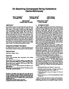
Figure 2.1 Examples of various range searching query types in two dimensions. (a) Simplex. (b) Halfspace. (c) Dominance (2-sided). (d) Circular. (e) Orthogonal (4-sided). (f) 3-sided. (g) Parabolic. . . . . . . . . . . . .
13
Figure 2.2 (a) An example K-set (K = 4) in R2 and a separating line. (b) An example of a 2-dimensional aboveness reporting query. . . . . . . . .
17
Figure 2.3 (a) A point p with a level of 3. (b) The K-level of an arrangement of lines (K = 3). (c) The (≤ K)-level of an arrangement of lines (K = 3). 18 Figure 2.4 Planar point location: identifying the face of a planar subdivision containing the query point q. . . . . . . . . . . . . . . . . . . . . . . . .
22
Figure 4.1 Order-1 Hilbert lattice . . . . . . . . . . . . . . . . . . . . . . . . . .
33
Figure 4.2 Building the order-2 Hilbert lattice . . . . . . . . . . . . . . . . . . .
33
Figure 4.3 First four iterations of the Hilbert curve. . . . . . . . . . . . . . . . .
34
Figure 4.4 First three iterations of the Peano curve. . . . . . . . . . . . . . . . .
34
Figure 4.5 Entry and exit points of the 2 dimensional Hilbert curve (the x-axis corresponds to the least significant bit and the y-axis the most significant). . . . . . . . . . . . . . . . . . . . . . . . . . . . . . . . . . . .
41
Figure 4.6 Running algorithm HilbertIndex with n = 2, m = 3 and p = [5, 6].
47
Figure 4.7 Comparing performance over random data-sets. (a) Time to calculate N indices with m = 4 as n varies. (b) Time to calculate N indices with n = 4 as m varies. . . . . . . . . . . . . . . . . . . . . . . . . . .
58
Figure 4.8 A comparison of dynamic Hilbert sorting and compact Hilbert sorting using the WEBLOG data-set. The compact curve includes the cost of converting both to and from compact Hilbert indices. (a) Wall times. (b) Relative speed-up. . . . . . . . . . . . . . . . . . . . . . . . . . .
59
Figure 5.1 (a) The recursive construction of the point set. Fat solid lines bound grid cells, dotted lines separate subcolumns. (b) The set of queries in QT . Only one query is shown for each level of QT . (c) Queries at recursive levels output only points from their subgrids. . . . . . . . .
66
viii
� � Figure 5.2 (a) An O N(log log N)1/α -space layout for the point set S (layout shown for α = 3). (b) Answering a query on the first two levels of the layout. The dark portion of the query in each copy of S forms a contiguous subsequence of the column-major layout of the respective group. The light portion is answered using subsequent copies of S. . .
75
Figure 5.3 (a) Replacing 3-sided queries with parabolic ones. The white squares are the areas where the subgrids in each grid cell are to be placed. (b) A naively constructed query in the subgrid in cell T3,6 also reports points in other cells (e.g., T2,6 ). (c) Placement of a subgrid within a grid box G that is nested inside a column box C. (d) Incremental embedding of a subgrid T � inside a grid box. . . . . . . . . . . . . . .
80
Figure 6.1 (a) An arrangement of lines. The shaded region, excluding its boundary is a 2-dimensional cell. The fat line segment excluding its endpoints is a 1-dimensional cell. The highlighted vertex is a 0-dimensional cell. (b) The lower envelope of the arrangement is shaded dark gray. The (≤ 2)-level includes all light gray and all dark gray faces. (c) The regions bounded by fat lines are a shallow cutting for the (≤ 2)-level of the arrangement. (d) The fat lines belong to the conflict list of the shaded cell. . . . . . . . . . . . . . . . . . . . . . . . . . . . . . . . .
89
Figure 6.2 Illustration of the query procedure in the proof of Lemma 6.2. Thin solid lines show the top boundaries of some (≤ 2j )-levels. The shallow cutting Ci with i = �log K � � is shown using fat dashed lines. The ˜ C of the cell C ∈ Ci containing the query approximate conflict list Δ point q contains the fat solid curves crossing C but not the thin ones, solid or dashed. . . . . . . . . . . . . . . . . . . . . . . . . . . . . . .
92
Figure 6.3 Two levels of the recursive structure for polylogarithmic queries. The entire structure consists of of an approximate counting structure D for polynomial queries over F , a point location structure L(C) for the shallow cutting C of the (≤ N 1−δ /2c )-level of F , as well as structures constructed recursively for the cells C1 , C2 , C3 of C. The representation of each cell Ci consists of an approximate counting structure Di for polynomial queries over ΔCi , a point location structure L(Ci ) for a shallow cutting Ci of ΔCi , as well as structures constructed recursively for the cells of Ci , indicated by the different shading of cells. Note that, even though the shallow cuttings define a recursive partition of space, this does not necessarily produce a partition of F . For instance, if the structure represents an arrangements of lines, the line � would be represented in the data structures of all three cells C1 , C2 , and C3 and of some sub-cells of C2 and C3 . . . . . . . . . . . . . . . . . . . .
97
ix
Figure 6.4 For queries above the (N 1−δ /2c )-level, Db is used to answer the query. For queries between the (logτ N)-level and the (N 1−δ /2c )-level, Ds is used. For queries between Cs and Cb , L(Cb ) is used to locate the cell C ∈ Cb containing the query point, and the final answer is obtained using DC . For queries contained in Cs , L(Cs ) is used to locate the cell C � ∈ Cs containing the query point, and the final answer is obtained by scanning ΔC � . . . . . . . . . . . . . . . . . . . . . . . . . . . . . . 100 Figure 6.5 Reduction of dominance queries to aboveness queries in 2-d. (The construction in 3-d is identical, except that the last step requires two 45◦ -rotations.) (a) A point set (white) and a query range defined by the black corner point q. Points p1 and p2 are contained in the query range; p3 is not. (b) Piecewise linear functions corresponding to the white points. q is a above the functions defined by query points p1 and p2 , but not above the one defined by p3 . (c) Rotating the figure 45◦ to the left makes all functions totally defined and does not change aboveness. . . . . . . . . . . . . . . . . . . . . . . . . . . . . . . . . . 102
x
Abstract This thesis focuses on range searching data structures, an elementary problem in computational geometry with research spanning decades. These problems often involve very large data sets. Processor speeds increase faster than memory speeds, thus the gap between the rate at which CPUs can process data and the rate at which it can be retrieved is increasing. To bridge this gap, various levels of cache are used. Since cache misses are costly, algorithms should be cache-friendly. The input-output (I/O) model was the first model for constructing cache-efficient algorithms, focusing on a two-level memory hierarchy. Algorithms for this model require manual tuning to determine optimal values for hardware dependent parameters, and are only optimal at a single level of a memory hierarchy. Cache-oblivious (CO) algorithms are built without knowledge of the hierarchy, allowing them to be optimal across all levels at once. There exist strong theoretical and practical results for I/O-efficient range searching. Recently, the CO model has received attention, but range searching remains poorly understood. This thesis explores data structures for CO range counting and reporting. It presents the first space and worst-case query-time optimal approximate range counting structure for a family of related problems, and associated O(N log N)-space query-optimal reporting structures. The approximate counting structure is the first of its kind in internal memory, I/O and CO models. Researchers have been trying to create linear-space query-optimal CO reporting structures. This thesis shows that for a variety of problems, linear space is in fact impossible. Heuristics are also used for building cache-friendly algorithms. Space-filling curves are continuous functions mapping multi-dimensional sets into one-dimensional ones. They are used to build search structures in the hopes that objects that were close in the original space remain close in the resulting ordering. This results in queries incurring fewer page swaps when traversing the structure. The Hilbert curve is notably good at this, but often imposes a space or time penalty. This thesis introduces compact Hilbert indices, which remove the ineffiency inherent for input point sets with bounding boxes smaller than their bounding hypercubes.
xi
List of Abbreviations and Symbols Used
[·][2]
Used to denote non-negative integers written in base 2
�·�
Number of ‘1’ bits in the binary representation of a non-negative integer (the parity)
∨
Bitwise or operator
⊕
Bitwise exclusive-or operator
∧
Bitwise and operator
�
Bitwise not-and operator
¬
Bitwise not/negation operator
�
Bitwise shift-left operator
�
Bitwise shift-right operator
�
Bitwise left-rotation operator
�
Bitwise right-rotation operator
2-d
Two-dimensional
3-d
Three-dimensional
B
Memory block size
B
A set of block sizes
B
Set of boolean integers {0, 1}
B(P )
Smallest n-dimensional box Bm0 ×· · ·×Bmn−1 such that P ⊆ B(P )
B-cover
A block cover
Bk
Set of positive integers of k bits, Z2k
bit (a, k)
Represents the value of the kth bit of a non-negative integer a
CO
Cache-oblivious
CPU
Central processing unit
d
A direction in Zn xii
d(0), . . . , d(2n − 1)
Sequence of directions in Zn such that e(i) ⊕ 2g(i) ⊕ 2d(i) = e(i + 1)
ε
A small positive quantity
e
An entry point in Bn
e(0), . . . , e(2n − 1)
Sequence of entry points in Bn
f
An exit point in Bn
f(0), . . . , f(2n − 1)
Sequence of exit points in Bn
FIFO
First in, first out
g(0), . . . , g(2n − 2)
Sequence of integers in Zn such that gc(i) ⊕ 2g(i) = gc(i + 1)
gc
Binary reflected Gray code function
gcr
Gray code rank function
GIS
Geographic information system
h
A Hilbert index in BM
H(P )
Smallest n-dimensional hypercube Bm × · · · × Bm such that P ⊆ H(P )
I
An indexing scheme
I/O
Input-output
K
Number of reported points/output size
L1
Level 1
L2
Level 2
L3
Level 3
LRU
Least-recently used
LV
Las Vegas xiii
M
Size of main memory
m
Maximum precision, m = maxi {mi }
m0 , . . . , mn−1
Precision (number of bits) of each of the n dimensions
MC
Monte-Carlo
μ
A mask in Bn
N
Number of points/problem size
N
Set of natural integers, {0, 1, . . .}
n
Number of dimensions
n-d
n-dimensional
P
A set of points
p = [p0 , . . . , pn−1 ]
A point in the space B(P )
perm(N)
External permutation complexity Θ(min sort(N), N)
Q
A set of queries/subsets of S or P
q
A query
R
Set of real numbers
RAM
Random access memory
S
A set
sort(N)
� � External scanning complexity Θ N � B log M External sorting complexity Θ N B
T(e,d) (b)
Hilbert curve transformation function
tsb
Trailing set bits function
scan(N)
B
xiv
N B
�
U = {u0 < . . . < u�μ�−1 }
Set of unconstrained bits associated with a given mask μ
W
A workload
WC
Worst-case
X
Net precision, X =
Z
Set of integers, {. . . , −1, 0, 1, . . .}
Z+
Set of positive integers, {1, 2, . . .}
Zk
Set of integers modulo k, {0, . . . , k − 1}
xv
� i
mi
Acknowledgements During my work on this thesis I had the honour and pleasure of being supervised by Norbert Zeh, whose depth of knowledge came to my rescue on many occasions. I am also in debt to his dedication and invaluable guidance; he always had time to discuss new ideas and to review drafts, even while dealing with the upheaval of a sabbatical on another continent. Without his intellectual input, this work would have been impossible. I would also like to thank Peyman Afshani whose own thesis work brought to light the key insight allowing the main results of this thesis to unfold after almost two years of fruitless efforts. I extend thanks to my committee members Andrew Rau-Chaplin and Alex Brodsky for their willingness to work through this thesis in detail, providing valuable feedback. I thank NSERC, the Killam Foundation, Norbert Zeh and Dalhousie University for their generous financial support without which my continued studies would have been an impossibility. I wish also to thank my friends at Dalhousie for making my time there memorable, specifically Mason Macklem, Glenn Hickey and Greg Zaverucha. They were always ready to talk about new ideas, and more importantly, to take my mind off of research when required. My family deserves my gratitude for their continued encouragement and support. Specifically, my sister Sara Hamilton whose own doctoral journey provided me with much needed context and motivation. Last but not least, my partner Caroline Pich´e has been with me through this entire process. She has coped with my distracted nature when buried in work, all the while wearing a smile. Her love and easy laughter has been a much needed source of energy and inspiration day after day.
xvi
Chapter 1 Introduction 1.1
Motivation
This thesis focuses on the development of algorithms and data structures for cache-efficient range searching. Range searching problems are among the most natural problems in computational geometry. As a consequence, they are among the most well-studied. Range searching exists in many forms (What space does the problem live in? What is being reported? What is the shape of the query regions?), with most variants finding practical applications. For example, orthogonal range searching problems are directly motivated by queries in database systems, while circular range searching queries find immediate use in geographic information systems (GIS). Many seemingly unrelated problems may also be reduced to range searching problems through appropriate geometric reductions, as will be discussed in more detail in Chapter 2. Practical applications of range searching problems often involve extremely large data sets, particularly in the domains of database systems and GIS. This creates unique challenges. Computer systems have evolved to contain numerous layers of data storage (on-processor storage, RAM, hard-disk, network, etc), with layers further away from the processor typically having greater capacities but slower access times. Processor speeds have been increasing faster than memory speeds, thus the gap between the rate at which CPUs can process data and the rate at which data can be loaded from memory is constantly increasing. To bridge this gap, various levels of cache were introduced. In fact, modern computers typically have at least six such layers (L1, L2, L3, RAM, hard-drive cache, hard-drive itself). The hope is that most memory accesses can be served from the nearest cache. For most algorithms, this is not true. Since cache misses are quite expensive, it becomes extremely important for algorithms to manage data in a cache-friendly manner. The cost of a cache miss is smaller the higher up the hierarchy it occurs, as memory speeds increase as we climb the hierarchy. An obvious first approach is to minimize cache misses at the slowest level, but a good algorithm will be one that is simultaneously efficient across all levels in a cache hierarchy. 1
2 The input-output (I/O) model was the first model for designing cache-efficient algorithms. It ignores the higher levels of cache and only distinguishes between data stored in memory and that stored on the disk. In this manner, it minimizes cache misses at the single level of the hierarchy where they incur the largest cost. Algorithms designed in this model explicitly control the swapping of data between the two levels, and implementations require manual tuning to determine optimal values for what are essentially hardware dependent parameters. The cache-oblivious (CO) model is a simple abstraction that allows the construction of cache-friendly algorithms without specific knowledge of the cache hierarchy. In the CO model algorithms are designed without referencing parameters of the model hierarchy, however, they are analyzed as in the I/O model. This abstraction means that the analysis holds for any memory hierarchy parameters, and thus simultaneously across all levels of a multi-level memory hierarchy. The I/O and CO models will be discussed in more detail in Section 2.1. The database and GIS communities have long recognized the importance of cacheefficiency, with several I/O-efficient algorithms finding real application in these domains [21, 34,68]. In particular, the problem of range searching has been well studied in the I/O model, with excellent practical results [27,68,119]. In the last decade, CO algorithms have received a lot of attention from the computational geometry community, however the problem of range searching is still poorly understood with many open questions. Another approach to building cache-friendly algorithms is the use of various tried and proven heuristics [61, 106, 109]. Space-filling curves are continuous self-similar functions that map compact multi-dimensional sets into one-dimensional ones. They are commonly used in the creation of range searching data structures in the hopes that objects that are close in the original space remain close in the resulting one-dimensional data structure [51,75,78], usually a type of search tree. The end result is that leaves containing a point in a query very likely contain other points belonging to the same query. Thus, queries need to visit fewer leaves in the resulting data structure, and fewer page swaps are incurred. The Hilbert curve has been shown as being particularly well suited to this task [100]. However, depending on the specifics of their use, Hilbert curves impose either a space or time penalty. This thesis solves this problem with compact Hilbert indices, which remove the inefficiency inherent in Hilbert indices for input point sets with bounding boxes significantly smaller than their bounding hypercubes. Although this thesis focuses on Hilbert curves, many other space-filling curves exist [72].
3 1.2
Overview
This thesis focuses on cache-efficient range searching, with a focus on axis-aligned range searching problems. The work is divided into two parts. The first part discusses heuristics for data locality in range searching structures. Specifically, Chapter 4 presents a practical improvement to Hilbert index calculations and evaluates its real-world utility. The second part of this thesis focuses on results in the cache-oblivious model. While both the CO model and the problems we discuss are practically motivated, the results presented in the latter part of this thesis are purely theoretical. Chapter 5 discusses lower bound results for range searching in the CO model, while Chapter 6 discusses data structures for range searching in the CO model.
1.2.1
Hilbert curves
In Chapter 4 we explore the Hilbert curve, reproducing classical algorithms [39, 43] for their generation and manipulation through an intuitive and rigorous geometric approach. We then extend these basic results to construct compact Hilbert indices which are able to capture the ordering properties of the regular Hilbert curve but without the associated inefficiency in representation for data sets whose bounding boxes are significantly smaller than their bounding hypercubes. Consider a set P of points in Zn . For simplicity and without loss of generality, we assume that the point set has been translated such that all coordinates are positive, and the bounding box has one corner at the origin. The points in P lie within a power-of-two-sided bounding box B(P ) = [0, 2m1 ] × · · · × [0, 2mk ] (letting mi ∈ N be the minimum values such that this is true) and therefore can be naturally represented using � X = i mi bits. However, the Hilbert curve is naturally defined over a power-of-two-sided bounding hypercube H(P ) = [0, 2m ]×· · ·×[0, 2m ], where m = maxi (mi ), with each position on the curve encoded by an mn-bit integer. For many real world data sets mn is significantly larger than X. By considering only the portion of the curve intersecting B(P ), compact Hilbert indices allow the ordering of the Hilbert curve to be preserved while only using X bits to represent each position on the compact curve. This leads to reductions in spacebounds for algorithms with precomputed Hilbert indices, or reductions in computation time for algorithms that repeatedly calculate the Hilbert index as needed. In particular, these results provide the first optimal time in-place Hilbert-order sort for multi-dimensional data
4 sets whose power-of-two-sided bounding boxes are smaller than their power-of-two-sided bounding hypercubes. Our main technical contribution in this chapter is in the creation of compact Hilbert curves, generalizations of Hilbert curves that are naturally defined over B(P ) rather than H(P ). 1.2.2
Lower bounds
The focus of Chapter 5 is on 3-sided range reporting, 3-d dominance reporting, and 3-d halfspace range reporting. We prove the novel result that any cache-oblivious data structure for these problems that achieves the optimal (or in fact a much weaker) query bound has to use asymptotically more space than a structure with the same query bound in the I/O model. There exist linear- and O(N log∗ N)-space data structures that achieve the optimal query bound of O(logB N + K/B) for these range searching problems in the I/O model [2, 7]. In contrast, the best known data structures achieving the same query bound in the cache-oblivious model use O(N log N) space [13, 25, 30]. Our lower bound shows that any cache-oblivious data structure for 3-sided range reporting, 3-d dominance reporting or 3-d halfspace range reporting that achieves a query bound of f (logB N, K/B), for any monotonically increasing function f (·, ·), has to use Ω(N(log log N)ε ) space. The only previously existing separation results between these two models are for sorting and searching. The sorting result used an adversarial argument over only two discrete block sizes [64]; the searching result applies in the limiting sense over many block sizes, but results in only a constant factor separation result [36]. Our approach is novel in that it is an explicit construction that argues simultaneously across many block sizes and yields the first input-size-dependent separation result between the I/O and cache-oblivious models. 1.2.3
Upper bounds
Chapter 6 focuses on the construction of a generic approximate range counting and range reporting data structure. Early I/O-efficient data structures for orthogonal range reporting are based on fairly direct externalizations of internal-memory data structures and techniques [12, 24, 107]. These approaches generally involve nested structures, where non-trivial secondary search structures are embedded in the nodes of a B-tree, with each secondary structure being queried on a root-to-leaf path. However, the entire technique of non-trivial secondary data structures breaks down in the CO model as it is impossible to ensure they
5 are cache aligned for all possible values of B. This incurs a page swap per accessed secondary data structure, resulting in a non-optimal O(log N)-cost search tree traversal. More recent I/O-efficient data structures employ shallow cutting and shallow partitions [7], but require explicit knowledge of B. Shallow partition techniques require the indexing of multiple secondary data structures and as such do not appear promising in a CO context. Chapter 6 shows how to exploit shallow cuttings to guarantee data locality in a cache-oblivious manner, something that has not been previously done. Investigations into 3-sided range searching techniques yielded the insight that existing data structures in the I/O and CO model use an approach reminiscent of shallow cuttings [30]. Shallow cuttings being more general and powerful, this led to the development of a unifying framework that can additionally handle 3-d halfspace and 3-d dominance queries. The results are constructions for O(N log N)-space cache-oblivious data structures with optimal query bounds across a family of problems. In the case of 3-sided range reporting, the results match those previously obtained in [13,25,30], but they are the first of their kind for the problems of 3-d halfspace, circular, 2-d K-nearest neighbour and 3-d orthogonal range reporting. These reporting data structures are fairly easy to obtain using a standard construction once the output size of a query can be efficiently determined or at least approximated. Our main technical contribution is a general framework for constructing cache-oblivious data structures for the approximate counting versions of the above problems. These data structures use linear space and provide guaranteed relative (1+ε)-approximate answers using O(logB (N/K)) block transfers in the worst case, which is optimal. This is in contrast to previous results even in internal memory, where the optimal query bound was not achieved in the worst case before, even using superlinear space. The only previous data structure with the optimal query bound, by Afshani and Chan [6], achieves this bound only in the expected case. Thus, our construction also provides new worst-case optimal data structures for approximate 3-d halfspace range counting and approximate 3-d dominance counting in the pointer machine model. Tables 3.1 and 3.2 contrast our results with previous work.
Chapter 2 Preliminaries In this chapter we introduce the common terminology, notation and concepts that will be used throughout this thesis. Definitions that apply only to particular chapters or sections will be provided as needed. 2.1
Models of Computation
Since the analysis of algorithms from an I/O-complexity point of view is not as well established as the analysis of their running time or their space requirements, we dedicate a few pages to the discussion of various models of computation. We discuss the relationship between external memory models and internal memory algorithms, allowing the comparison between existing algorithms for the problems we consider and our algorithms. 2.1.1
The Random Access Machine Model
The most commonly studied internal memory model is the random access machine (RAM) model. Algorithms designed for this model execute instructions sequentially and all operations are performed on data items stored in a conceptually unlimited main memory. Valid instructions consist of elementary arithmetic and logical operations, instructions to read and write data from or to memory and control instructions allowing the realization of branching, looping and recursion. Each elementary operation is assumed to take O(1) time on a data item representable by O(log N) bits, where N is the size of the input. Thus, in order to estimate the amount of time necessary for an algorithm to solve a given problem, it suffices to count the number of steps executed by the algorithm. A number of variants to this model have been proposed, most of which can be distinguished based on the set of operations that are considered primitives of the machine. Since most operations in more powerful RAM models can be emulated at a small (although nonconstant) cost in a weaker RAM model, these variations are of little relevance to us, as computation cost is ignored in the analysis of external memory algorithms. 6
7 We will be confining ourselves to the standard algebraic model of computation, which allows only multiplication, division, addition and subtraction as primitive arithmetic operations. In particular, the floor function is not considered a primitive of this model, although it may be emulated in O(log N) time. The geometric algorithms discussed in this thesis will generally (unless stated otherwise) be assuming that the fundamental machine words are real numbers. This avoids the hassle of dealing with precision problems. However, these issues must be addressed when actually implementing these algorithms1 . In the real world the size of main memory is limited and it is possible that the problem does not fit entirely in memory. In this case, it is possible for every read or write operation to cause data to be swapped between main memory and external memory (disk). Since a memory swap incurs significant cost (orders of magnitude slower than a primitive computation operation as permitted by the model [120, 121]), it is possible for optimal RAM algorithms to perform very poorly when realized on actual hardware. The following sections discuss models of computation that attempt to address this issue.
2.1.2
The Input-Output Model
The first widely accepted and used model for analyzing the complexity of algorithms in external memory was the I/O model of Aggarwal and Vitter [21]. This model considers two levels of memory: a single processor is equipped with a slow but conceptually unlimited disk (external memory), and a fast random access memory (internal memory) capable of holding M data items. The disk is partitioned into blocks of B consecutive data items. The processor may only perform computations on items held in internal memory. In order to access other data, the processor must first make room in the internal memory by transferring data items to the external memory or discarding it if no longer needed, at which point it may then load the desired data items into internal memory. Such memory transfers are called I/O operations or block transfers. In a single block transfer, the processor may shuttle one block of data items from external memory to internal memory, or vice-versa. The complexity of an algorithm in the I/O model is the number of block transfer it performs. The I/O model explicitly ignores the time taken by the processor to perform any required computations. This is motivated by the fact that access times to a hard-disk are about six 1 Obviously, care must be taken not to abuse the model by exploiting the infinite storage capacity of actual real numbers.
8 orders of magnitude slower than a computation step [120, 121]. An algorithm that performs fewer block transfers can be expected to be faster than one performing more block transfers, assuming the amount of computation performed by the first remains within reasonable bounds. Despite this fact, most I/O model algorithms are designed using the algebraic computation model, and thus may be analyzed in terms of RAM model complexity as well. In fact, it is entirely possible (and often the case) that algorithms exist which are optimal in both the I/O and RAM models simultaneously. The I/O model has been widely adopted because it is a conceptually simple model that captures the main bottleneck in large-scale computations. The simplicity of the model has been important to its success as it allows relatively complicated problems to be explored and solved. Moreover, it typically results in solutions that can actually be implemented and yield real-world performance improvements over internal memory models. The disadvantage of this model is that the parameters M and B are essentially hardware dependent, and implementations must be optimized for each individual machine on which the code is to be run.
2.1.3
The Cache-Oblivious Model
The I/O model of computation only consider two levels of a memory hierarchy. However, modern computers typically have many memory levels, each higher level being faster yet also smaller than the previous. An example of such a hierarchy is the following: network storage, local disk, disk cache, RAM, L2 CPU cache, L1 CPU cache. The straight-forward extension of the I/O model to a multi-level hierarchy would require the addition of a blocksize parameter between each neighboring pair of levels in the hierarchy. Design and analysis of algorithms in such a model quickly becomes cumbersome. Over the years, various parameterized models have been proposed for handling multi-level cache hierarchies [20, 22], but they have proven unwieldy. Frigo et al. proposed an elegant model avoiding this problem [64]: the cache-oblivious (CO) model. In their model, the algorithm is oblivious of the memory hierarchy and, thus, cannot initiate block transfers explicitly. Instead, the swapping of data between two levels of memory is the responsibility of a paging algorithm, which is assumed to be offline optimal. That is, it performs the minimum number of block transfers possible for the memory access sequence of the algorithm. Such a paging algorithm will elect to evict the block of memory
9 which will be accessed the furthest in the future. Clearly, it is impossible to know this at runtime, so real-world caches typically use simpler cache eviction policies: • Least-Recently Used (LRU). Evict the block which was last accessed the longest time ago. • First In, First Out (FIFO). Evict the block which has been in the cache the longest. Sleator and Tarjan [114] showed that both LRU and FIFO are within a constant factor of the optimal strategy. More precisely, they showed that cost(LRU or FIFO cache with size 2M ) ≤ 2 × cost(optimal cache with size M ), where ‘cost’ counts the number of incurred block transfers. For most algorithms, changing M by a constant factor incurs at most a constant factor penalty, thus we may generally assume an optimal paging strategy, justifying use of the model. Algorithms in this model are thus designed as internal memory algorithms, but analyzed in the I/O model with respect to an arbitrary block size B. Since the memory parameters are used only in the analysis, the analysis may be applied to any two consecutive levels of the memory hierarchy. In particular, if the analysis shows that an algorithm is optimal with respect to two levels of memory, then it is simultaneously optimal at all levels of the memory hierarchy. As with the I/O model, it is possible to design algorithms that are optimal in both the RAM model and the CO model, and as an immediate consequence, the I/O model as well. Much as the I/O model, the CO model has seen success because it is conceptually simple enough to allow the study of hard problems. Remark. While motivated by practical considerations, the CO model has yet to find much in the way of real-world applications; the few algorithms that have been implemented rarely perform better than their I/O-model counterparts [41]. Those algorithms that have not been implemented, including the results of Chapter 6, use complex constructions that would likely incur very large constant factors. 2.2
Space-Filling Curves and Data Locality
Space-filling curves are continuous one-to-one functions which map a compact interval to a multi-dimensional unit hypercube. Originally formulated by Giuseppe Peano in 1890 [103],
10 the first space-filling curve was constructed to demonstrate the somewhat counter-intuitive result that the infinite number of points in a unit interval has the same cardinality as the infinite number of points in any bounded finite-dimensional set. In this thesis we are specifically interested in their application to database systems, particularly orthogonal range queries.
Since Peano introduced the first space-filling curve, numerous others have been constructed and extensively studied. Among these further developments is the family of curves generated by Hilbert [74], which to this day finds many applications. Due to the recursive geometric nature of the original construction, the Hilbert curve naturally imposes an ordering on the points in finite square grids. An ordering with data locality is a one-dimensional ordering of the points in a set P ⊆ Zn such that points that are close in the original space tend to remain close in the one-dimensional ordering. The end result is that leaves containing a point in a query very likely contain other points belonging to the same query. Thus, queries need to visit fewer leaves in the resulting data structure, and fewer page swaps are incurred. The Hilbert curve has been shown to be particularly well suited to this task [100].
While algorithms designed in the I/O and CO models attempt to rigorously categorize cache performance, space-filling curves are used as a heuristic to improve the cache performance of simple internal memory algorithms. The very popular R-tree data structure [68] (and its many variants) was initially conceived as a spatial variant to B-trees for orthogonal range queries in n dimensions. In a standard R-tree, data points are clustered into B sets of similar size with each set being represented in the search tree by its minimum bounding box. The division is repeated recursively until leaves contain roughly B points. The end result is a standard B-tree structure over potentially overlapping bounding boxes. Axis-aligned spatial queries are easily propated through the data structure, allowing efficient queries. Variants of the R-tree typically play with the method in which points are clustered into individual boxes at each step of the recursive division, how the boxes themselves are ordered and stored, as well as the details of how insertions and deletions are performed. Space-filling curves can be used to both segment data and order individual boxes, resulting in improved cache performance [78].
11 2.3
Notation
When discussing I/O-efficient and cache-oblivious algorithms we will use N to denote the size of the problem (number of data items), B to denote the block size and M to denote the number of data items that fit in internal memory. The use of K will be reserved for output-sensitive algorithms, and denotes the number of data items produced in the output or the actual value of the output when it is a single scalar value. When discussing range searching problems, we will generally use P to refer to a set of points in Rn , with n being reserved to indicate the dimensionality of the problem. The point set P is the input to such problems, thus it follows that N = |P |. Similarly, we will generally use q when referring to a query over P , where q is a query of the type admissible by the range searching problem being considered. We reserve Q to represent a set of queries and Q to represent the set of all valid queries admitted by the problem. When discussing complexity, ε will always refer to a small positive constant. For two values a and b, if a ≥ (1 − ε)b, then we say a is ε-approximately greater than b. Similarly, if a ≤ (1 + ε)b, then we say a is ε-approximately less than b. If both conditions hold, we say that a is ε-approximately equal to b. We will also occasionally use the notation Oε (·) to hide constant factors that depend on ε. Although asymptotic notations can more properly be thought of as representing sets of functions, we will occasionally abuse the notation slightly. For example, rather than writing 4x2 + x ∈ O(x2 ) we will write 4x2 + x = O(x2 ). Similar usage will be made of Θ(·), Ω(·), etc. We will occasionally make use of the following shorthands for the I/O-complexities of sorting, permuting and scanning a list of N data items: � � N N log M , sort(N) = Θ B B B perm(N) = Θ(min(sort(N), N)), � � N . scan(N) = Θ B
and
These shorthands have been introduced in the literature because they arise frequently in the analysis of I/O algorithms. Scanning and sorting are fundamental operations in many algorithms. In particular, external memory algorithms often sort the input data appropriately, before scanning the elements and processing them one by one. Equivalent internal memory algorithms do not
12 require such preprocessing as the elements may be accessed in a random fashion without any performance penalty. These I/O complexities also have important and obvious relations to well-known timecomplexities in internal memory. In particular, sort(N) is the external memory equivalent of the Θ(N log N) time bound for sorting N data items. As such, if a problem can be solved in O(N log N) time in internal memory, we hope to be able to solve it in O(sort(N)) I/Os in external memory. Similarly, the above scanning bound is the external memory equivalent of linear scanning in internal memory. Hence, we will refer to scan(N) as a linear number of I/Os, while O(N) I/Os is considered to be superlinear. This is a natural interpretation as any external memory algorithm spending O(N) I/Os does not utilize the full bandwidth of the I/O system. Finally, the permutation bound is interesting as it is superlinear, while permutation in internal memory takes linear time. This is interesting in that it provides a first separation result between the internal- and external-memory models. It also implies that a superlinear external-memory lower bound can be shown for many non-trivial problems that can be solved in linear time in internal memory, simply because these problems inherently encapsulate some permutation problem. 2.4
Definitions
In this section we introduce standard definitions and conventions used in the range searching literature. In particular, we precisely define the various range searching problems that will be addressed in later chapters. 2.4.1
Range Searching Problems
Consider a set P of points in Rn ; the problem of geometric range searching is to (efficiently) preprocess P so that, for any given query range q, information regarding the points in P ∩ q can be efficiently reported. The exact nature of this information depends on the type of range searching problem. In range reporting, we are interested in efficiently enumerating all of the points P ∩ q. In range counting, we are interested in reporting the size of the intersection, |P ∩q|. Range emptiness problems are decision problems where we are interested in determining if the query range q contains at least one point. Finally, range optimization problems are interested in finding a single best point in the query range with respect to some criterion (i.e., that with the largest weight, or with the smallest y coordinate, etc).
13
(a)
(b)
(e)
(c)
(f)
(d)
(g)
Figure 2.1: Examples of various range searching query types in two dimensions. (a) Simplex. (b) Halfspace. (c) Dominance (2-sided). (d) Circular. (e) Orthogonal (4-sided). (f) 3-sided. (g) Parabolic. In the context of Hilbert curves, we will assume that P consists of points in Zn , translated such that all coordinats are positive and the minimum bounding box includes the origin. We will also make extensive reference to various bounding boxes containing P . Consider the smallest bounding box [0, s1 − 1] × · · · × [0, sd − 1] containing P and the origin. The side lengths of this bounding box are si , each requiring mi = �log2 si � bits to represent. We define B(P ) := [0, 2m1 ] × · · · × [0, 2md ] to be the smallest power-of-two-sided bounding box containing P . Let m = maxi (mi ), and define H(P ) := [0, 2m ] × · · · × [0, 2m] as the smallest power-of-two-sided bounding hypercube containing P . As will be discussed in Chapter 4, the Hilbert curve through a set P is naturally defined over the (sometimes much) larger space H(P ). It is usually the case that Q is restricted to a specific class of geometric objects. A few important types of geometric range searching include the following (see Figure 2.1 for example queries): • Simplex range searching: In this problem, the query object q is a simplex, a convex hull in Rn formed by n + 1 points. Since any polyhedral object can be decomposed into simplices, the simplex case is a fundamental problem.
14 • Parabolic range searching: Here we limit ourselves to query regions consisting of the points lying on and above a parabola in Rn . • Circular (spherical) range searching: In this problem, the query regions are circles (hyperspheres) of arbitrary radius in R2 (Rn ). Problems of this type are regularly encountered in GIS (geographic information systems). As an example, consider the task of finding all restaurants within a given radius of a given location. • Orthogonal range searching: Here the query objects are orthogonal boxes. Many problems outside computational geometry can be reduced to this case. The canonical example arises naturally in the context of databases. Consider the problem of finding all employees aged between x1 and x2 who earn a salary between y1 and y2 . If employees are represented as points in R2 , then this query amounts to reporting all points lying in the orthogonal range [x1 , x2 ] × [y1 , y2 ]. In two dimensions, we often refer to orthogonal range searching as 4-sided range searching. Similarly, the case where y2 = ∞ is referred to as 3-sided range searching. • Dominance range searching: Here the query range is defined by a single point a ∈ Rn , and the query region consists of the points of Rn that are smaller than a in each coordinate. In two dimensions, this is the same as 2-sided range searching. Using standard reductions, solutions to this problem can be used to construct efficient solutions to 3-sided and orthogonal range searching [4, 5]. Additionally, 3-sided range searching can be reduced to 3-d dominance searching via a simple geometric transformation (see Lemma 2.1). • Halfspace range searching: In this problem the query object is a halfspace. Algorithmically, a halfspace may be considered as a simplex with one vertex placed sufficiently far away and thus this is a special case of simplex range searching. However, considered on its own it often allows more efficient specialized solutions. It is also interesting because both spherical range searching and parabolic range searching in Rn reduce to halfspace range searching in Rn+1 via elementary geometric transformations (see Lemmas 2.2 and 2.3). There are a variety of other range searching problems, and different ways to classify them. We limit ourselves to the above problem types, but more complete lists may be found in [12,
15 59, 96]. For most range reporting problems in up to 3 dimensions the optimal internal memory query bound is O(log N + K), with the log N corresponding to the cost of a search in some data structure and the K being the cost of reporting the K items that lie in the given query range. In external memory the natural cost of reporting K items is scan(K) = K/B. An information theoretic argument shows that the natural search cost is logB N. Consider a search tree with N possible outcomes. Specifying a single leaf in this tree requires lg N +O(1) bits of information. A comparison yields exactly 1 bit of information, yielding the lg N +O(1) lower bound on the number of comparisons necessary to navigate the tree. However, each block read reveals where the query element lies with respect to B elements in the tree, providing at most lg B + O(1) bits of information. Thus the number of block reads is at least (lg N + O(1))/(lg B + O(1)) = logB N + O(1), yielding an optimal range reporting query bound of Ω(logB N + K/B). As mentioned above, it is often the case that a range searching problem of one type may be transformed to a range searching problem of another type. In fact, there exist simple geometric transformations that allow 3-sided range queries to be decomposed into 3-d dominance queries, 2-d parabolic queries to be mapped to 3-d halfspace queries, and circular range searching queries to be mapped to 3-d halfspace queries. Similarly, these results can easily be lifted to higher dimensions. Lemma 2.1 (3-sided ⊂ 3-d dominance). Three-sided range queries can be solved by a data structure for 3-d dominance queries. Proof. Consider a 3-sided range query [x1 , x2 ] × [y1 , ∞). We transform points using the mapping p �→ (−px , px , −py ), and consider 3d-dominance queries of the form q = (−x1 , x2 , −y1 ). The transformed point is dominated by the query point if and only if −x1 ≥ −px
and x2 ≥ px
and
− y1 ≥ −py ,
which is equivalent to x1 ≤ px ≤ x2
and y1 ≤ py .
This is exactly the condition required for the original point to fall within the original 3-sided query.
16 Lemma 2.2 (2-d parabolic ⊂ 3-d halfspace). Parabolic range searching problems in R2 may be solved by a data structure for halfspace range searching in R3 . Proof. A point p = (px , py ) is on or above a query parabola with equation s(x − x0 )2 + y0 if and only if py ≥ s(px − x0 )2 + y0 . Consider the halfspace defined by {(x, y, z) ∈ R3 : ax + by + cz + z0 ≤ 0}. We transform points with the map p �→ (px , py , p2x ). Letting the halfspace be parameterized by the 4-tuple (a, b, c, z0 ), we transform queries with the map (s, x0 , y0) �→ (−2sx0 , −1, s, sx20 + y0 ). In this setting, a point (px , py , p2x ) lies in the halfspace if and only if 0 ≥ −2sx0 px − py + sp2x + sx20 + y0 py ≥
s(p2x − 2x0 px + x20 ) + y0
py ≥
s(px − x0 )2 + y0 .
This is equivalent to the point (px , py ) lying above the parabola defined by the 3-tuple (s, x0 , y0 ). Lemma 2.3 (Circular ⊂ 3-d halfspace). Circular range searching queries may be solved by a data structure for halfspace range searching in R3 . Proof. Consider a circular range searching query consisting of the circle of radius r centered at the point c = (cx , cy ) ∈ R2 . A point p = (px , py ) lies within this query if and only if (px − cx )2 + (py − cy )2 ≤ r 2 . Consider mapping the point p to a point in R3 via the mapping p �→ (px , py , p2x + p2y ), and consider mapping a query circle q = (c, r) to the halfspace parameterized by (c, r) �→ (−2cx , −2cy , 1, c2x + c2y − r 2 ).
(2.4)
17 A point lies in this halfspace if and only if −2cx px − 2cy py + p2x + p2y + c2x + c2y − r 2 ≤ 0 (p2x − 2cx px + c2x ) + (p2y − 2cy py + c2y )
≤ r2
(px − cx )2 + (py − cy )2
≤ r2,
which is exactly Equation 2.4. Straight-forward extensions to Lemmas 2.2 and 2.3 allow the construction of similar lemmas over Rn . Since many fundamental range searching problems have strong connections to halfspace range searching, this problem is of particular importance. Many interesting results on halfspace range searching make use of the natural notion of geometric duality [59], as will be explored in the following section. 2.4.2
Levels
The concept of levels arises quite naturally when studying problems that deal with sets of points or arrangements of hyperplanes in Rn . The concept was first explored by Lov´asz [89] and Erd˝os [62]. They defined a K-set for a set P of N points in the plane as a subset of P of size N that can be separated from the rest of P by a line (see Figure 2.2(a) for an example). Bounding the maximum number of K-sets as a function of N and K is known as the K-set problem. The concept of K-sets can be extended to higher dimensions through the use of separating hyperplanes. Point-hyperplane duality is a well-known elementary geometric transformation that preserves the spatial relationship between points and hyperplanes [59]. We represent the dual ¯ Through this duality, of a geometric object s (or a set S of geometric objects) with q¯ (or S). a point p below a hyperplane h is mapped to a hyperplane p¯ which passes strictly below ¯ Thus, a subset of points of P below a hyperplane h corresponds to a subset the point h. ¯ This problem can be thought of as the of hyperplanes of P¯ passing below2 the point h. (hyperplane) aboveness reporting problem, an example of which is shown in Figure 2.2(b). Given an arrangement of hyperplanes A in Rn , we define the level of a point p as the number of hyperplanes passing directly below p (as demonstrated in two dimensions in 2 In this context, below can be more precisely defined as P¯ passing through the half-ray extending vertically ¯ downwards from the point h.
18
(a)
(b)
Figure 2.2: (a) An example K-set (K = 4) in R2 and a separating line. (b) An example of a 2-dimensional aboveness reporting query.
(a)
(b)
(c)
Figure 2.3: (a) A point p with a level of 3. (b) The K-level of an arrangement of lines (K = 3). (c) The (≤ K)-level of an arrangement of lines (K = 3).
Figure 2.3(a)). Consequently, the K-level of A is the closure of the set of all points of A with level equal to K (see Figure 2.3(b)). The size of the K-level is the number of vertices of A contained in it. In dual space, the K-set problem asymptotically translates to bounding the size of the K-level of A. This is known as the K-level problem. Research into K-levels has led to many useful generalizations. Many results can be applied to the K-levels of pseudo-lines or pseudo-halfplanes as well. An arrangement of x-monotone curves is called an arrangement of pseudo-lines if every two curves intersect at most once. There are many papers dealing with such generalizations in the plane [15, 16, 18, 19, 47, 48, 50, 91, 104, 115, 116]. Similar generalizations for convex or concave hypersurfaces in
19 higher dimensions have received some attention [49, 83, 113]. These generalizations all have associated aboveness reporting problems. In many applications it is more convenient to talk about (≤ K)-levels, the closure of the set of all points of Rn with level at most K (see Figure 2.3(c)). The 0-level is often referred to as the lower envelope of an arrangement A. The term complexity is used interchangeably with size when referring to K- and (≤ K)-levels. It is relatively easy to construct arrangements where every K-level of A has size Θ(N). Thus, Ω(NK) is an obvious lower bound on the worst case size of the (≤ K)-level and a matching O(NK) upper bound can be proved. Here we present a short proof based on the randomized techniques of Clarkson and Shor [57]. To use this technique we need surprisingly few elementary tools and an upper bound on the 0-level of the arrangement. In two dimensions, the worst case complexity of the 0-level is O(N). Lemma 2.5 ( [57]). The complexity of the (≤ K)-level of an arrangement A formed by a set P of N lines in the plane is O(NK). Proof. Let S be a random p-sample of P (a subset of P where each element is chosen independently with probability p). Let L0 be the 0-level of the arrangement formed by S. Fix p := K −1 . We have
�
� N E[|L0 |] = O(Np) = O . K
(2.6)
Let C be the set of all the vertices contained in the (≤ k)-level of A. We compute the probability of a vertex v ∈ C appearing on the lower envelope of S. Let l� and l�� be the two lines incident to v, and let l1 , . . . , lt be the lines which pass below v. Since we have assumed that v lies inside the (≤ K)-level of A, we must have that t ≤ K. The probability of v appearing on L0 is equal to the probability of l� and l�� being chosen in S times the probability that none of the lines l1 , . . . , lt are chosen in S. Since t ≤ K we have � � � � Pr[v ∈ L0 ] ≥ p2 (1 − p)K = Θ p2 e−Kp = Θ K −2 . Thus, it follows that E[|L0 |] = Ω(|C|K −2 ). Combining with Equation 2.6 we have � � N −2 |C|K = O , K or equivalently, |C| = O(NK).
20 This is a fundamental upper bound on (≤ K)-level complexity. In three dimensions, the worst case complexity of the lower envelope is O(N) and the same technique yields the following bound, stated here without proof. Lemma 2.7. The complexity of the (≤ K)-level of an arrangement A formed by a set P of N hyperplanes in R3 is O(NK 2 ). 2.4.3
Cuttings and Partitions
The divide-and-conquer technique is fundamental to the design of many successful algorithms. Cuttings provide a natural way to divide a geometric problem into balanced and bounded subproblems. Let H be a set of N hyperplanes in Rn . A 1/r-cutting of H is a set of disjoint simplices C which cover H such that each simplex s ∈ C intersects at most N/r hyperplanes of H. For a simplex s ∈ C, we call the subset of H intersecting s the conflict list of s and we denote it by Δs . The size of the cutting is the number of simplices in C. The main cutting theorem is the following, due to Chazelle [54, 55]. Theorem 2.8 (Cutting Theorem [54, 55]). For every parameter 0 < r < N, there exists a 1/r-cutting of size O(r n ) for a set H of hyperplanes in Rn . The bound O(r n ) on the size of the cutting is tight: N hyperplanes form Θ(N n ) vertices and a simplex intersecting m hyperplanes can contain at most O(mn ) vertices of an arrangement. So each simplex in a 1/r-cutting contains O((N/r)n ) vertices and thus, there must be Ω(N n /(N/r)n ) = Ω(r n ) simplices in the cutting. Consider a set P of N points in Rn . A simplicial partition Π for P is a partition of P into r subsets P1 , . . . , Pr of roughly the same size together with a list of simplices s1 , . . . , sr such that Pi lies inside si . The crossing number of any hyperplane h in this simplicial partition is defined as the number of simplices crossed by h. The maximum value of the crossing number over all hyperplanes h is called the crossing number of Π. When constructing simplicial partitions, it is desirable (from a data structure point of view) that the crossing number of the partition be minimized. Matouˇsek was the first to construct an optimal simplicial � � partition of P [93], where the crossing number is O r 1−1/n . Both cuttings and partitions are useful in building divide-and-conquer data structures for aboveness reporting problems [7, 95, 96]. Partitions are space efficient in that every hyperplane is found in exactly one of the subsets. However, each hyperplane has a relatively
21 high crossing number, forcing us to look at multiple secondary data structures as we recurse down the search tree. Cuttings take the opposite approach; by oversampling the hyperplanes, super-linear storage space is required but only one substructure needs to be queried as we descend the search tree. Both approaches work in internal memory, but partitions require the indexing of too many secondary data structures in external memory models. As such, cuttings (and particularly shallow cuttings) have received more attention in these models. 2.4.4
Shallow Cuttings
In certain contexts, ‘shallow’ versions of the cutting and the partition theorem can be formulated, as originally noticed by Matouˇsek [94]. In the shallow version of the cutting theorem we are not partitioning the entire space. Rather, for parameters K and r a K-shallow 1/rcutting for a set P of hyperplanes is a set of disjoint simplices C which cover the (≤ K)-level of P , and where each simplex c ∈ C intersects at most N/r hyperplanes of P . While any ordinary cutting is a shallow cutting, better size bounds are obtainable for shallow cuttings. Lemma 2.9 (Existence of shallow cuttings, [94]). For a set P of hyperplanes in Rn and � � parameters r and K < N, a K-shallow 1/r-cutting of size O r n (K/N)�n/2� always exists. The above lemma is usually most useful when r = N/K. Applying this and a few other modifications results in the following 3-d variant of the lemma. Lemma 2.10 (Lemma 1.1.6 of [3]). For any set of N planes in R3 and a parameter K, there exists a K-shallow O(K/N)-cutting of size O(N/K) that covers the (≤ K)-level. The cells in the cutting are all vertical prisms unbounded from below (simplices with one vertex at (0, 0, −∞)). Furthermore, we can construct these cuttings for all K of the form �(1 + ε)i � simultaneously in Oε (N log N) time. The conflict lists may also be constructed in this time. Outline of proof. The first part follows from Lemma 2.9. The construction time follows from an algorithm by Ramos [108]. The fact that vertical prisms suffice was observed by Chan, and converting to an equivalent prism shallow cutting requires computing the convex hull of the vertices in the original shallow cutting [45]. To compute the conflict lists we begin by building a halfspace range reporting data structure in Oε (N log N) expected time. For each K we issue O(N/K) halfspace range reporting queries (one per prism vertex), each
22 requiring Oε (log N + K) time, for a total of Oε (N(log N + K)/K). Summing this over all K gives Oε (N log N). Finding simplices that are all prisms allows us to easily construct a data structure for querying the level of a point. Consider one level of the cutting. Project the prisms on the xy-plane, yielding a triangulation composed of O(N/K) faces. Each face of the triangulation stores the equations of the plane corresponding to the top face of its vertical prism. For any point q ∈ R3 we can easily find the face containing the point’s projection on the xy-plane using a planar point location data structure. For a triangulation containing N faces, such a structure can be built in O(N log N) time and O(N) space, answering queries in O(log N) time. Thus, in O(log(N/K)) time we can test whether q lies below a given level of the cutting and if so, determine the vertical prism containing it.
Remark. It is worth noting that the proofs relating to shallow cuttings are merely existence results, and say nothing about actually building them. The actual algorithms used for constructing shallow cuttings (such as that by Ramos [108]) are directly descended from the powerful randomized techniques of Clarkson and Shor [57]. Thus, while many data structures based on shallow cuttings have deterministic run times, they only have expected bounds on the preprocessing required to actually build them.
2.4.5
Planar Point Location
Point location problems are natural and well-studied problems in computational geometry. Consider a set S of n-dimensional objects in Rn ; the point location problem consists of efficiently preprocessing S so that, for any given query point p ∈ Rn , the objects s ∈ S such that p ∈ s can be efficiently reported. The problem may be simplified by forcing the objects to be simplices, forcing them to be disjoint, and/or forcing them to completely cover the entire space (or some defined portion of it). Given a planar subdivision, planar point location consists of finding the unique cell that contains a given query point q (see Figure 2.4). As hinted at in the proof outline of Lemma 2.10, planar point location structures can be helpful in building and manipulating data structures based on shallow cuttings. As such, they are useful in the construction of data structures for solving various range searching problems, as will be seen in Chapter 6. Arge et al. developed an optimal data structure for planar point location in the CO model [29]
23
Figure 2.4: Planar point location: identifying the face of a planar subdivision containing the query point q.
which we will use in our data structures.
Chapter 3 Previous Work 3.1
Hilbert Curves
The uses of Hilbert curves are wide and varied, including mathematics [42], image processing [86, 122], image compression [99], bandwidth reduction [102], cryptology [92], algorithms [105], scientific computing [51,76], parallel computing [23,77], geographic information systems [1] and database systems [38, 78, 88]. A large variety of algorithms exist for computing the Hilbert curve [33, 39, 42, 43, 75, 87, 101, 117], each directed towards a particular application. In the context of databases and GIS, Butz’s classic algorithm [43] is the most commonly used, whose standard implementation was created by Thomas [117] and later refined by Moore [101]. The algorithms are all equivalent in complexity, requiring a number of operations proportional to the number of bits output in the Hilbert index, and vary only in their details. Butz’s algorithm is presented rather cryptically, introducing seven layers of subscripted variables in order to describe the algorithms in terms of fundamental bitwise boolean logic operations. The algorithm proved popular because it uses very little state, and is easily implemented non-recursively for increased performance. Moore [101] later refined Butz’s algorithm to remove the dependency on lookup tables. Lawder [87] cleaned up the presentation of these algorithms and formally extended them to higher dimensions. However, all of these presentation obscure the high level operations that are actually occurring: rotations, reflections and Gray code calculations. In Chapter 4 we reproduce Butz’s algorithm from a geometric point of view, casting the bit operations in terms of these high level concepts. Bartholdi [33] concentrates specifically on the rotations and translations that occur when descending through the levels of recursion, maintaining orientation information using algebraic transition functions. Their techniques generalize to other families of space-filling curves, but they are meant explicitly for forward and reverse index calculations, and do not efficiently allow enumerations of the curve. Jin and Mellor-Crumley [75] trade space for speed and precalculate all possible inputs and outputs of the state transition function. Their techniques allow for efficient traversal of 24
25 arbitrary space-filling curves, as well as for efficient forward and reverse index calculations. However, they require separate lookup tables for each possible dimension, and thus do not gracefully handle arbitrary dimensions. The popularity of Moore’s approach in the context of databases is due to its seamless handling of arbitrary dimensions. For domains with a fixed number of dimensions, techniques using precomputed lookup tables or state transition functions are more efficient [75]. In the context of range searching, Hilbert curves have found use as a sort order in a variety of spatial data structures [68,78,88,100,101]. Since the Hilbert curve is naturally defined over a bounding hypercube H(P ) that is typically much larger than the bounding box B(P ) of the input points P , converting the points to Hilbert indices requires an increase in space usage. To combat this, Moore [101] developed Hilbert index comparison routines that compute the Hilbert indices of two points simultaneously bit-by-bit, stopping when the relative order can be determined. This introduces an expected O(log N)-cost per comparison [63], resulting � � in a sub-optimal expected O N log2 N -time sort algorithm. Another approach to solving this problem is to remove the inefficiency in representation of Hilbert indices. The results presented in Chapter 4 take this approach, by generating compact Hilbert indices for points sets where B(P ) is smaller than H(P ). Our results are the first to generalize Hilbert curves to ‘rectangular’ sets B(P ), and as a corollary, produce the first optimal Hilbert sorting algorithm for points in B(P ). The key insight necessary for this construction was made possible by revisiting Butz’s algorithm from a geometric point of view.
3.2
Lower Bounds
In internal memory most range searching problems have been rather fully explored and optimal algorithms found. This includes 2- and 3-d orthogonal range reporting (and its 2and 3-sided variants in the plane) [59, 98], 3-d dominance reporting [2, 90] and 3-d halfspace range reporting [7]. A notable exception to this general rule is for exact halfspace range � � counting in the plane where only an Ω N 1−1/n / log N query lower bound is known for linear space data structures [53], but the best known data structure (believed to be optimal) � � requires O N 1−1/n query time [93]. In the plane, the lower bound sharpens to the optimal �√ � Ω N , but the log factor for higher dimensions is thought to be an artifact of the proof technique.
26 In the I/O model, Arge et al. [28] showed that Θ(N logB N/ logB logB N) space is sufficient and necessary to obtain a query bound of O(logB N + K/B) block transfers for 2-d orthogonal range reporting. This lower bound, when applied to blocks of size N ε , implies that achieving the optimal query bound cache-obliviously requires Ω(N log N) space.
Lower bound proofs for range reporting problems in the I/O model [28, 73, 85, 110] have involved the construction of a hard point set together with a set of many ‘sufficiently different’ queries of the same size. Combined with counting arguments from extremal set theory, this ensures that the point set cannot be represented in linear space while guaranteeing a certain proximity (on disk) of the points reported by each query. Such lower bound results immediately carry over into the cache-oblivious model, but they are unable to be made stronger in the CO model because they inherently discuss only a single query size. Our results are distinct in that they require arguing simultaneously over many different query sizes. This necessitates the use of new techniques as those from extremal set theory no longer apply.
There have been very few lower bound results in the cache-oblivious model, but the results that have been found show that the CO model is inherently less powerful than the I/O model. In [40], Brodal and Fagerberg established a lower bound on the amount of main memory (as a function of B) necessary for optimal cache-oblivious sorting. They showed that sorting in optimal O(sort(N)) time is only possible under the tall cache assumption, namely that M = Ω(B 1+ε ). Since sorting is such a fundamental technique underlying many more complicated data structures this assumption is often made in the CO literature. The result used an adversarial argument over two block sizes. Such a technique is doomed to failure for range searching lower bounds as we can build data structures that are optimal for any constant number of block sizes. In [36], Bender et al. proved that cache-oblivious searching has to cost a constant factor more than the search bound achieved in the I/O model using B-trees [34]. Their result applies in the limiting sense over many block sizes. Our results are unique in that they are the first to establish a gap between the two models that grows with the input size of the problem, and the first to use an explicit construction that argues simultaneously across many block sizes.
27 3.3
Upper Bounds
In internal memory, linear-space data structures with the optimal query bound of O(log N + K) are known for 3-sided range reporting [98], 3-d dominance reporting [2,90], and 3-d halfspace range reporting [7], as well as for a number of related problems. Using the reductions of Section 2.4.1, the results for halfspace range reporting imply the same results for 2-d parabolic, circular, and 2-d K-nearest neighbour reporting. Exactly counting the number of points in a query range seems significantly harder than reporting if the query bound is to be independent of the output size K. For 3-sided range counting Chazelle [52] obtained a linear-space data structure with query time O(log N), which also � � immediately implies an O(N log N)-space data structure with query time O log2 N for 3d dominance counting. For exact 3-d halfspace range counting, Matouˇsek [95] obtained a � � linear-space data structure with a query bound of O N 2/3 , and this is conjectured to be the best possible. As a result, much effort has been put into obtaining approximate halfspace range counting structures with polylogarithmic query bounds. Aronov and Har-Peled [31] presented a general technique that can be used to construct an approximate range counting structure from one for range emptiness queries; the obtained data structure provides a correct approximation of the number of points in the query range with high probability. The cost of this transformation is an increase of the space bound by a factor of log N and an increase of the query bound by a factor of log N log log N. For halfspace range searching, linear-space range emptiness structures with O(log N) query time have been known for a long time (see, for example, [84]). Thus, the technique by Aronov and Har-Peled provides an O(N log N)-space approximate halfspace range counting � � structure with a query time of O log2 N log log N . Kaplan and Sharir [82] improved the query time by a factor of log log N using an interesting combinatorial lemma concerning the overlay of lower envelopes in a randomized incremental construction (see also [80, 81]). Like Aronov and Har-Peled, they were able to guarantee correctness only with high probability. Later, Aronov and Har-Peled showed in an updated version of their paper [32] that an � � O log2 N query time can be obtained using O(N log N) space without applying the overlay lemma. Har-Peled and Sharir [71] showed that a worst-case query time of O(log N log log N) � � O(1) N space. This was improved by Afshani and Chan [6], can be achieved using O N log who presented a linear-space data structure with the same worst-case query bound, as well as another linear-space data structure that uses the overlay lemma to achieve the optimal
28 query time of O(log(N/K)) in the expected case. The fact that the overlay lemma is a crucial component of Afshani and Chan’s optimal data structure has a number of limiting implications: the method does not generalize to other problems, unless a similar overlay lemma is proved for each such problem; a nontrivial modification of the overlay lemma would be required to use it in models such as the I/O model or the cache-oblivious model; and, finally, it cannot be used to obtain a worstcase query bound. The other methods discussed above have similar shortcomings in that they are tailored to internal-memory models or to specific problems. For example, many of the log N-factors in the above complexity bounds are the result of applying Chernoff-type inequalities (completely independent of B) and cannot easily be reduced to logB N in the I/O model or the cache-oblivious model. Our range counting results are notable in that they are the first to achieve worst-case optimal queries in linear space (a first even in internal memory), and they generalize to a variety of problems for which no previous approximate range counting results were previously known. In the I/O model, much work has focused on orthogonal range reporting. A number of linear-space data structures have been proposed that achieve a query bound of � � � � N/B + K/B block transfers in 2-d and O (N/B)1−1/n + K/B block transfers in n O dimensions [27, 66, 67, 79, 106, 109]. In [28], Arge et al. showed how to achieve a query bound of O(logB N + K/B) for 3-sided range reporting in the plane, using linear space. They also showed that Θ(N logB N/ logB logB N) space is sufficient and necessary to achieve a query bound of O(logB N + K/B) block transfers for general 2-d orthogonal range reporting. The main tool used to prove the 3-sided upper bound is a linear-space I/O-efficient version of McCreight’s priority search tree [98] with a query bound of O(logB N + K/B) for 3-sided queries. For 3-d dominance reporting, Vengroff and Vitter [119] presented a data structure with a query
bound
of
O((log log logB N) log(N/B) + K/B)
O(N log(N/B)) space in the I/O model.
block
transfers
and
using
The query bound can be reduced to
O(logB N + K/B) by choosing the parameters in the data structure more carefully [120]. A recent data structure by Afshani [2] achieves the optimal query bound of O(logB N + K/B) block transfers using linear space, raising the question whether this result can be achieved in the cache-oblivious model. This data structure also yields a 3-d orthogonal range reporting � � structure that uses O N log3 N space and achieves the same query bound.
29 Halfspace range reporting in 3-d has a longer history, in part because it generalizes various other range searching problems, as was discussed in Section 2.4.1. In internal memory, Chan described an O(N log N)-space data structure with an expected query time of O(log N + K) [44]. Building on these ideas, Agarwal et al. [14] obtained an O(N log N)space data structure with an expected query bound of O(logB N + K/B) block transfers in the I/O model. Further research led to the development of internal-memory data structures with the optimal query bound in the worst case and using O(N log log N) space [46,108]. The same improvements can be carried over to the I/O model. Recently, Afshani and Chan [7] described a linear-space data structure with the optimal query bound in internal memory and an O(N log∗ N)-space data structure that answers queries using O(logB N + K/B) block transfers in the I/O model. Much less is known in the cache-oblivious model. Orthogonal range reporting queries in � � Rn can be answered using O (N/B)1−1/n + K/B block transfers [13, 26]. Cache-oblivious range reporting structures with a query bound of O(logB N log log N + K/B) block transfers and using O(N log N) space are easily obtained for 3-d halfspace and 3-d dominance queries using existing techniques [59]. Thus, the interesting questions are whether cacheoblivious data structures for these problems exist that achieve the optimal query bound of O(logB N + K/B) block transfers and how much space is necessary to achieve this bound. For 3-sided queries, data structures with the optimal query bound and using O(N log N) space were proposed in [13, 25, 30]. The data structure by Arge and Zeh [30] was obtained using a standard reduction to 2-d dominance queries, for which the paper presented a linearspace data structure with the optimal query bound. The data structure by Arge et al. [25] can be seen as being based on some notion of shallow cuttings for 3-sided range searching, combined with a specialized 2-d dominance counting structure. For the remaining problems, such as 3-d dominance reporting and 3-d halfspace range reporting as well as their approximate counting versions, no non-trivial results were previously known in the cacheoblivious model. Our range reporting results are distinct in that they unify similar previous approaches, and generalize to a variety of range searching problems for which no equivalent results were previously known.
30 Query type 3-d halfspace
Model RAM
Space
Query bound 2
References
N log N N log N
log N log log N log2 N
(MC) (MC)
N logO(1) N N N
log N log log N log N log log N log(N/K)
(WC) (WC) (LV)
Aronov, Har-Peled 2005 [31] Aronov, Har-Peled 2005 [31] Kaplan 2006 [82] Kaplan, Sharir 2007 [80] Kaplan, Sharir 2011 [81] Aronov, Har-Peled 2005 [31] Afshani, Chan 2009 [6] Afshani, Chan 2009 [6]
3-d halfspace
RAM I/O & CO
N N
log(N/K) logB (N/K)
(WC) (WC)
new new
3-d dominance
RAM I/O & CO
N N
log(N/K) logB (N/K)
(WC) (WC)
new new
Table 3.1: A comparison of our results on approximate range counting with previous work. In the listing of query bounds, WC refers to worst-case bounds; LV to Las Vegas bounds, that is, query bounds that hold in the expected sense; and MC to Monte Carlo bounds, that is, the answer to a query is correct with high probability. For the sake of clarity, O-notation has been omitted.
Query type
Model
Space
Query bound
References
2-d 3-sided
RAM I/O CO
N N N log N
log N + K logB N + K/B logB N + K/B
McCreight 1985 [98] Arge 1999 [28] Agarwal 2003 [13] Arge, Brodal 2005 [25] Arge, Zeh 2006 [30] Afshani, Hamilton, Zeh 2009 [9]
3-d dominance
RAM
N
log N + K
I/O CO
N N log N
logB N + K/B logB N + K/B
Makris 1998 [90] Afshani 2008 [2] Afshani 2008 [2] new
RAM I/O CO
N N log∗ N N log N
log N + K logB N + K/B logB N + K/B
Afshani, Chan 2009 [7] Afshani, Chan 2009 [7] new
3-d halfspace
Table 3.2: A comparison of our results on range reporting with previous work. For the sake of clarity, O-notation has been omitted.
Chapter 4 Compact Hilbert Indices
In the first part of this chapter we recreate Butz’s classic algorithm [43] for Hilbert curves, but from a geometric point of view. This intuitive approach allows for a deeper level of understanding of the primitives used in Butz’s algorithm, at the same time providing insight into other algorithmic approaches such as Bartholdi and Goldsman’s vertexlabelling approach [33] and Jin and Mellor-Crummey’s table-driven methods [75]. Consider H(P ) = [0, 2m ] × · · · × [0, 2m ], the power-of-two-sized bounding hypercube of P . By considering the order in which the Hilbert curve visits the points in H(P ) we may assign an index between 0 and 2mn − 1 to each point. In other words, positions on the curve are naturally encoded by an mn-bit integer. In the context of database systems this enumeration can be used to sort the points in P while preserving data locality. This in turn translates to data structures with excellent range query performance [78, 100]. In the real world, point sets do not have such ideal distributions and consequently the bounding box B(P ) = [0, 2m1 ] × · · · × [0, 2mn ] may be significantly smaller than the bounding hypercube H(P ). Coordinates along the ith dimension require mi bits to represent, thus � points in B(P ) can be represented using X = i mi bits. In the second part of this chapter we explore the notion of compact Hilbert indices, which assign to points an index requiring exactly X bits to represent. This is done by only considering the portion of the Hilbert curve intersecting B(P ). This may be done trivially by calculating the Hilbert index of each point B(P ), sorting them based on this index, and then simply assigning indices in 0 through 2X − 1. However, such an approach requires an exhaustive enumeration of B(P ). The approach we discuss in this chapter can generate such an index for a single point of B(P ) in absence of any others. The algorithms presented in this chapter were implementd in the form of a C++ library for the computation of both regular and compact Hilbert curves and indices. In the third part of this chapter we evaluate the performance of this library and validate the utility of compact Hilbert indices. 31
32 The most important contribution of this chapter is in the development of compact Hilbert indices. The geometric reconstruction of Butz’s algorithm is only necessary to gain sufficient insight into the mechanics of the algorithm, allowing us to remove the redundant computation and space requirements of ordinary Hilbert indices. No previous work attempts to generalize space-filling curves to non-hypercube lattices. The results of this chapter were published in [69, 70].
4.1
Hilbert Curves
We begin by building the necessary tools for the exploration of Hilbert curves. We take a geometric approach, yielding algorithms that are identical to those of Moore [101]. Moore’s algorithms are refinements based on Thomas’s implementation [117] of Butz’s classic algorithm [43]. The terminology and notation used in this section is largely my own, and I have chosen to deviate from existing convention in order to highlight the geometric approach taken here, and the relationship to standard boolean operators. The need for the level of detail in this construction will become apparent in the construction of algorithms for compact Hilbert indices in Section 4.2. We consider first the traditional recursive definition of the two dimensional Hilbert curve. For reasons that will become apparent later, we consider the Hilbert curve that starts in the bottom left corner and finishes in the upper left1 . The curve is initially defined on a 2 × 2 lattice, as shown in Figure 4.1. Given the order k curve2 defined on a 2k × 2k lattice, we may refine it to visit all points on a 2k+1 × 2k+1 lattice as follows: • Place a copy of the original curve, rotated counter-clockwise by 90◦ , in the lower left sub-grid. • Place a copy of the original curve, rotated clockwise by 90◦ , in the upper left sub-grid. • Place a copy of the original curve in each of the right sub-grids. • Connect these four disjoint curves in the one manner that uses only unit step sizes. 1 2
In the traditional presentation, the two-dimensional Hilbert curve finishes in the bottom right corner. The order k curve is the curve after k levels of recursion.
33 This construction may be visualized in Figure 4.2, with the first four iterations of the construction shown in Figure 4.3. In a completely analogous manner one may define the Peano curve, which travels through lattices of size 3k × 3k as shown in Figure 4.4.
Figure 4.1: Order-1 Hilbert lattice
Figure 4.2: Building the order-2 Hilbert lattice
Any finite-order two-dimensional Hilbert curve allows a simple mapping from 2 dimensions into 1, by simply associating a given grid point with its index along the curve. This same concept can be extended to arbitrary space-filling curves, as well as to higher dimensions. It is worth noting the fact that the Hilbert curves always take steps of unit length: immediate neighbors on the curve are also immediate neighbors in the plane. This translates to a notion of data locality: points close to each other in the plane tend to be close to each other along the Hilbert curve. 4.1.1
Higher Dimensions
The geometric approach to the two-dimensional Hilbert curve starts by considering a 2 × 2 grid of points and describes the path through them. It then recurses by replacing each point with another 2 × 2 grid (making a 22 × 22 grid) and defining the curve through each of those, appropriately rotated so that the entrance and exit points to these sub-grids remain adjacent. We consider an analogous recursive approach to the multi-dimensional Hilbert curve. Consider a grid of 2 × · · · × 2 points in n dimensions, corresponding to the corners of the unit hypercube in Zn . The key property of the Hilbert curve is that successive points are immediate neighbors in the grid. Thus, to maintain this property we are looking for a walk through the 2n points such that every point will be enumerated, and successive points will be neighboring corners of the hypercube.
34
(a)
(b)
(c)
(d)
Figure 4.3: First four iterations of the Hilbert curve.
(a)
(b)
(c)
Figure 4.4: First three iterations of the Peano curve.
35 We let each of the 2n vertices be labelled by an n-bit string of the form b = [βn−1 · · · β0 ][2] , where βi ∈ B := {0, 1} represents the position of the vertex along dimension i (0 for low, 1 for high). This is easily interpreted as an n-bit non-negative integer value in Z2n , or equivalently, Bn . Restricting ourselves to taking steps to immediate neighbors implies that in the binary labels of successive vertices, only one bit may change. In other words, we are looking for an ordering of the 2n distinct n-bit numbers such that any successive pair of numbers differ in exactly one bit. This corresponds exactly to the classic Gray code [65]. Gray Code In general, a Gray code is an ordering of numbers such that adjacent numbers differ in exactly a single digit with respect to some base. More specifically, we are concerned with a binary Gray code. Perhaps the simplest form of a binary Gray code is the binary reflected Gray code, which is intuitively constructed in the following manner: 1. Start with the Gray code over 1-bit numbers: [[0][2] , [1][2] ] 2. Write the sequence forwards and then backwards, prepending zeroes to the first half and ones to the second half. This creates the Gray code over all 2-bit numbers: [[00][2] , [01][2] , [11][2] , [10][2] ] 3. Repeat step 2, each time growing the Gray code over k-bit numbers to one over k + 1 bits. Assuming the input to step 2 is itself a Gray code over all k-bit numbers, it is easy to see that the output will be a valid Gray code over all (k + 1)-bit numbers. The 2-bit Gray code generated in this manner coincides exactly with the ordering through the four points in a two-dimensional Hilbert curve (it generates the familiar ‘�’ shape), and it can be used as a basis to extend the concept of the Hilbert curve to higher dimensions3 . Given this construction of the binary reflected Gray code, we may easily derive a closed form for the ith Gray code integer. The following results on Gray Codes are well known, but we have provided our own proofs for the sake of completeness. 3 This exact agreement is due to the non-standard orientation we have chosen for the Hilbert curve. Given the standard orientation, the agreement would only be up to a rotation.
36 Theorem 4.1 (Closed-form Binary Reflected Gray Code). The binary reflected Gray code sequence is generated by the function gc(i) = i ⊕ (i � 1), where ⊕ is the exlusive-or operator, and � is the right-shift operator. Proof. We consider the value of the jth bit of the ith Gray code, bit (gc(i), j). The construction begins with the Gray code sequence over B. After j iterations we have the Gray code defined over all (j + 1)-bit values. In this sequence, the first half of the values are defined such that the jth bit is zero, while the second half has a one for the jth bit. In the next iteration of this construction the pattern reverses itself such that (for 0 ≤ i < 4(2j )): ⎧ ⎧ j ⎪ ⎪ 0, if � 2ij � = 0, ⎪ ⎪ ⎪ 0, if 0 ≤ i < 2 , ⎪ ⎪ ⎪ ⎪ ⎪ ⎨ 1, if 2j ≤ i < 2(2j ), ⎨ 1, if � i � = 1, 2j bit (gc(i), j) = = j j ⎪ ⎪ 1, if 2(2 ) ≤ i < 3(2 ), 1, if � 2ij � = 2, ⎪ ⎪ ⎪ ⎪ ⎪ ⎪ ⎪ ⎪ ⎩ 0, if 3(2j ) ≤ i < 4(2j ) ⎩ 0, if � i � = 3. 2j In subsequent iterations of the construction this pattern will simply be repeated as it is already symmetric. Hence, it follows that for ⎧ ⎪ 0, ⎪ ⎪ ⎪ ⎪ ⎨ 1, bit (gc(i), j) = ⎪ 1, ⎪ ⎪ ⎪ ⎪ ⎩ 0,
all i ≥ 0 if � 2ij � mod 4 = 0, if � 2ij � mod 4 = 1, if � 2ij � mod 4 = 2, if � 2ij � mod 4 = 3.
i � mod 2 = 1 if and only if � 2ij � mod 4 ∈ {2, 3} we see that Since � 2j+1 ⎧ ⎪ 0, if � 2ij � mod 4 = 0, ⎪ ⎪ ⎪ ⎪ � � ⎨ 1, if � i � mod 4 = 1, i 2j + j+1 mod 2 bit (gc(i), j) = i ⎪ 2 � mod 4 = 2, 0, if � ⎪ j ⎪ 2 ⎪ ⎪ ⎩ 1, if � i � mod 4 = 3 2j � � � � i i = + j+1 mod 2 2j 2 = (i � j) + (i � (j + 1)) mod 2
= bit (i, j) + bit (i, j + 1) mod 2 = bit (i, j) ⊕ bit (i � 1, j) = bit (i ⊕ (i � 1), j) .
37 Thus it follows that gc(i) = i ⊕ (i � 1). Given a non-negative integer we may wish to find at which position it lies in the Gray code sequence. In other words, we may wish to determine the inverse of the Gray code. Theorem 4.2 (Binary Reflected Gray Code Inverse). Consider a non-negative integer i. Let m be the precision of i. That is, let m = �log2 (i + 1)� such that i requires m bits in its binary representation. Then it follows that bit (i, j) =
m−1 �
bit (gc(i), k) mod 2,
k=j
where bit (i, k) refers to the kth bit in the binary representation of i, with 0 being the least significant bit and m − 1 the most significant. Proof. By Theorem 4.1 we have bit (gc(i), j) = bit (i, j) + bit (i, j + 1) mod 2. Summing over j ≤ k < m we find that m−1 �
bit (gc(i), k) =
k=j
m−1 �
� � bit (i, k) + bit (i, k + 1) mod 2
k=j
=
�m−1 �
bit (i, k) +
k=j
= bit (i, j) +
m �
� bit (i, k)
mod 2
k=j+1
� 2
m−1 �
�
bit (gc(i), k)
+ bit (i, m) mod 2
k=j+1
= bit (i, j) + bit (i, m) mod 2. By the definition of m we see that bit (i, m) = 0 and the result follows. We use Theorem 4.2 to construct Algorithm 1, which computes the inverse as desired. Additionally, we are interested in knowing along which bit the Gray code will change when preceding from one term to the next. Equivalently, we are interested in knowing along which dimension we will step when proceeding from one vertex to another on the Hilbert curve. To this end, we define g(i) as g(i) = k, such that gc(i) ⊕ gc(i + 1) = 2k ,
0 ≤ i < 2n − 1.
38 Algorithm 1 GrayCodeInverse(g) Given a non-negative integer g, calculates the non-negative integer i such that gc(i) = g. Input: A non-negative integer g. Output: The non-negative integer i such that gc(i) = g. 1:
m ← number of bits required to represent g
2:
(i, j) ← (g, 1)
3:
while j < m do
4:
i ← i ⊕ (g � j)
5:
j ←j+1
6:
end while
Lemma 4.3 (Dimension of Change in the Gray Code). The sequence g(i) is given by g(i) = tsb(i), where tsb is the number of trailing set bits in the binary representation of i. Proof. We examine the difference between two consecutive values of the Gray code: gc(i) ⊕ gc(i + 1) = i ⊕ (i � 1) ⊕ (i + 1) ⊕ ((i + 1) � 1) = (i ⊕ (i + 1)) ⊕ ((i � 1) ⊕ ((i + 1) � 1)) = (i ⊕ (i + 1)) ⊕ ((i ⊕ (i + 1)) � 1). We consider first the portion i ⊕ (i + 1). Adding 1 to i will cause a carry past the first digit if the first digit is 1. Similarly past the second digit and so on. Letting k be the number of trailing ones in the binary representation of i (or, alternatively, the index of the first zero valued bit), it follows that i + 1 will have a one at position k, zeroes at positions 0 through k − 1, and be identical to i elsewhere. Thus, taking the exclusive-or of these two will result in a number with k + 1 trailing one bits. Similarly, the result of (i ⊕ (i + 1)) � 1 will be a number with k trailing one bits. Taking the exclusive-or of these two results in a number with a single non-zero bit at the kth position. Hence, between the ith and (i + 1)th Gray code integers it is the kth bit that changes. This corresponds exactly to the definition of ‘tsb’ thus it follows that g(i) = tsb(i). Lemma 4.4 (Symmetry of the Gray Code). Given n ∈ N and 0 ≤ i < 2n , it follows that gc(2n − 1 − i) = gc(i) ⊕ 2n−1 .
39 Proof. This property follows immediately from the construction algorithm for the reflected binary Gray code. The second 2n−1 values are simply equal to the first 2n−1 values in reverse, with the (n − 1)th bit set as a 1. Thus we see that gc(2n − 1 − i) = gc(i) ∨ 2n−1 , for 0 ≤ i < 2n−1 . Replacing the ‘or’ operation by an ‘exclusive-or’ (justified in this case as exaclty one of gc(2n − 1 − i) or gc(i) will have a zero in the (n − 1)th bit) leads to the desired result. Corollary 4.5 (Symmetry of g(i)). The sequence g(i) is symmetric such that g(i) = g(2n − 2 − i) for 0 ≤ i ≤ 2n − 2. Proof. Without loss of generality we consider i ≤
2n −2 . 2
Lemma 4.4 tells us that
gc(2n − 2 − i) = gc(i + 1) ⊕ 2n−1 . By the definition of gc we know that gc(i + 1) = gc(i) ⊕ 2g(i) and gc(2n − 2 − i) = gc(2n − n −2−i)
1 − i) ⊕ 2g(2
. Substituting these into the above equation yields n −2−i)
gc(2n − 1 − i) ⊕ 2g(2
= gc(i) ⊕ 2g(i) ⊕ 2n−1.
By Lemma 4.4 this simplifies to the desired result, g(2n − 2 − i) = g(i).
Analogous to the Hilbert curve in two dimensions, the Gray code ordering can be used to give an ordering through the vertices of a unit hypercube in Zn . As in the recursive construction in two dimensions, we will recursively define the Hilbert curve by zooming in on each point in the sequence (each sub-hypercube) and iterating through the points within using a transformed/rotated version of the original curve. Like the two-dimensional case, we must determine orientations for the Hilbert curve through each of the 2n sub-hypercubes. These orientations must be consistent in that the exit point of the curve through one subhypercube must be immediately adjacent to the entry point of the next sub-hypercube. Additionally, the entry and exit points of the parent hypercube must coincide with the entry point of the first sub-hypercube and the exit point of the last sub-hypercube, respectively. These constraints on entry and exit points are visualized for the two-dimensional case in Figure 4.5.
40 Entry Points Using the same labelling as the vertices of the parent hypercube, we let e(i) and f(i) refer, respectively, to the entry and exit vertices of the ith sub-hypercube in a Gray code ordering of the sub-hypercubes. Since the ith and (i + 1)th sub-hypercubes are neighbors along the g(i)th coordinate, we must have that f(i) ⊕ 2g(i) = e(i + 1). Like the entry and exit points of the parent hypercube, entry and exit points of a given sub-hypercube must be neighboring corners. That is, e(i) and f(i) may only differ in exactly one bit position, meaning we must have that e(i) ⊕ f(i) = 2d(i) for some d(i) ∈ Zn . We refer to d(i) as the intra sub-hypercube direction, and g(i) as the inter sub-hypercube direction. Combining these two results shows that entry points must satisfy the relation e(i + 1) = e(i) ⊕ 2d(i) ⊕ 2g(i) ,
0 ≤ i < 2n − 1.
(4.6)
Additionally, as mentioned earlier, we must have that e(0) is the same as the entry point of the parent hypercube and f (2n − 1) is the same as the exit point of the parent hypercube. These constraints are displayed graphically for the two-dimensional case in Figure 4.5. In order to fully determine closed forms for e(i), d(i) and f(i), we first explore various properties of these sequences. The process is guided by exploring a small two-dimensional example, as shown in Figure 4.5. From the symmetry of the Gray Code itself (an immediate consequence of its definition), we can infer similar symmetry relationships on the entry and exit corner sequences. This in turn allows us to infer the symmetry of the intra subhypercube direction sequence d(i). Aided by our small example, we can then posit a closed form that satisfies the symmetry constraint and the observed example values. The form of the hypothesis is then confirmed by verifying that it satisfies Equation 4.6. Lemma 4.7 (Symmetry of e(i) and f(i)). The sequences e(i) and f(i) are symmetric such that e(i) = f(2n − 1 − i) ⊕ 2n−1 . Proof. We consider walking through the Hilbert curve backwards, such that e¯i = f(2n −1−i) and the ith sub-hypercube is gc(i) = gc(2n − 1 − i). By Lemma 4.4 this is equivalent to gc(i) = gc(i) ⊕ 2n−1. Thus, it follows that f(2n − 1 − i) = e¯i = e(i) ⊕ 2n−1 . Corollary 4.8 (Symmetry of d(i)). The sequence d(i) is symmetric such that d(i) = d(2n − 1 − i) for 0 ≤ i ≤ 2n − 1.
41
f(3) = 10e(3) = 11
f(2) = 10
3
2 e(2) = 00 f(1) = 10
0
1
e(0) = 00f(0) = 01
i 0 1 2 3
e(i) [00][2] [00][2] [00][2] [11][2]
f(i) d(i) g(i) [01][2] 0 0 [10][2] 1 1 [10][2] 1 0 [10][2] 0 −
e(1) = 00
Figure 4.5: Entry and exit points of the 2 dimensional Hilbert curve (the x-axis corresponds to the least significant bit and the y-axis the most significant). Proof. Lemma 4.7 tells us that e(i) = f(2n − 1 − i) ⊕ 2n−1 and equivalently e(2n − 1 − i) = f(i) ⊕ 2n−1 . Combining these two yields e(i) ⊕ f(i) = e(2n − 1 − i) ⊕ f(2n − 1 − i). By the definition of d(i) we have that e(i) ⊕ d(i) = f(i) thus we see d(i) = d(2n − 1 − i).
Lemma 4.9. Suppose that
d(i) =
⎧ ⎪ ⎪ ⎨ 0,
i = 0;
g(i − 1) mod n, i = 0 mod 2; ⎪ ⎪ ⎩ g(i) mod n, i = 1 mod 2,
for 0 ≤ i ≤ 2n − 1. Then d(i) is symmetric as per Corollary 4.8. Proof. Suppose i = 0. Then d(0) = 0. Similarly, d(2n − 1) = g(2n − 1) = tsb 2n − 1 = n mod n = 0. Suppose i = 0 mod 2. Then d(i) = g(i − 1). Since 2n − 1 − i = 1 mod 2, we see that d(2n − 1 − i) = g(2n − 1 − i) = g(2n − 2 − (i − 1)) = g(i − 1). Suppose i = 1 mod 2. Then d(i) = g(i). Since 2n − 1 − i = 0 mod 2, we see that d(2n − 1 − i) = g(2n − 2 − i) = g(i). Thus, this form for d(i) meets the symmetry requirement of Corollary 4.8.
42 Theorem 4.10 (Intra Sub-hypercube Directions). The formula of Lemma 4.9 satisfies Equation 4.6, and hence defines the sequence of intra sub-hypercube directions, d(i). Proof. Let d(i, n) be the sequence of intra sub-hypercube directions for a fixed dimension n. By inspection (see Figure 4.5) we see that the above definition holds for the case n = 2. Suppose that the definition holds for 1, . . . , n and consider the case n+1. As long as g(i) < n, then g(i) mod n + 1 = g(i) mod n. Thus, we consider the first i such that g(i) ≥ n. By Lemma 4.3 we see that this occurs when i = 2n − 1, the smallest positive integer with n trailing set bits. Hence, for i < 2n − 1 we must have that d(i, n + 1) = d(i, n). Now consider d(2n − 1, n + 1). Since the exit point of the ith cell must touch the face of the (i + 1)th cell along the g(i)th axis, we must have that bit (f(i), g(i)) = bit (gc(i + 1), g(i)) . Substituting Equation 4.6 into this we must have that � �n n 2 −1
bit
⊕2
d(j,n+1)
⊕
2 −2
⊕2
j=0
g(j)
, g(2n − 1)
j=0
= bit
�
2n −1
⊕2
� g(j)
, g(2n − 1) ,
j=0
which simplifies to � bit � bit
2n −1
⊕2
� d(j,n+1)
, g(2n − 1)
j=0
2n −2
⊕2
d(j,n+1)
⊕2
d(2n −1,n+1)
⊕2
d(2n −1,n+1)
� , g(2n − 1)
j=0
� bit
2n −2
⊕2
= 1, = 1, �
d(j,n)
, g(2n − 1)
= 1.
j=0
By the symmetry of d(i, n) most of the first term cancels, leaving � � n bit 2d(0,n) ⊕ 2d(2 −1,n+1) , g(2n − 1) = 1. Since d(0, n) = 0 then we must have that d(2n − 1, n + 1) = g(2n − 1). We know that d(i, n + 1) holds for 0 ≤ 0 ≤ 2n − 1, and by Lemma 4.9 we know that this holds for the other half, 2n ≤ i ≤ 2n+1 − 1. Hence that definition holds for the case n + 1 and by the inductive hypothesis it holds for all n ≥ 2. With a closed form for d(i) we are able to determine the closed form for e(i).
43 Theorem 4.11 (Entry Points). The sequence of entry points is defined by � 0, i = 0, e(i) = �), 0 < i ≤ 2n − 1. gc(2� i−1 2 Proof. By recursive application of Equation 4.6 we have that i−1
e(i) =
⊕2
d(j)
j=0
⊕
i−1
⊕2
g(j)
.
j=0
By definition, for all n we have that e(0) = 0, thus we consider only the case i > 0. Simplifying the above yields e(i) = 2g(0) ⊕
i−1
⊕2
d(j)
⊕ gc(i)
j=1
⊕ 2d(1)� ⊕ �2d(2) �� ⊕ 2d(3)� ⊕ . . . ⊕ 2d(i−1) ⊕ gc(i). = 2g(0) ⊕ 2� d(0) �� Suppose i = 0 mod 2. Then by Theorem 4.10 all of the d(i) cancel out except d(i − 1), leaving us with e(i) = 2g(0) ⊕ 2d(i−1) ⊕ gc(i). Since g(0) = tsb(0) = 0 = tsb(i) = g(i) this �). yields e(i) = gc(i) ⊕2d(i−1) ⊕2g(i) = gc(i) ⊕2g(i−1) ⊕2g(i) = gc(i−2). Thus, e(i) = gc(2� i−1 2 Suppose now that i = 1 mod 2. All of the d(i) cancel, leaving e(i) = gc(i) ⊕ 2g(0) . Since g(0) = tsb(0) = 0 = tsb i − 1 = g(i − 1) this simplifies to e(i) = gc(i − 1). For i = 1 mod 2 �, hence e(i) = gc(2� i−1 �). we have that i − 1 = 2� i−1 2 2 Rotations and Reflections As noted in Section 4.1.1 the recursive construction of the Hilbert curve requires us to construct a curve through the corners of a hypercube when provided with a particular entry and exit point. The classic Gray code explored earlier starts at gc(0) = 0 and ends at gc(2n − 1) = 2n−1 , thus implicitly has an entry point e = 0, an internal direction d = n − 1 and an exit point f = 2n−1 . We wish to define a geometric transformation such that the Gray code ordering of sub-hypercubes in the Hilbert curve defined by e and d will map to the standard binary reflected Gray code. To this end, let us define the right bit rotation operator � as � � b � i = b(n−1+i mod n) · · · b(i mod n) [2] , where b = [bn−1 · · · b0 ][2] . Conceptually, this function rotates the n bits of b to the right by i places. Analogously, we define the left bit rotation operator, �. Trivially, both the left and right bit rotation
44 operators are bijective over Zn2 (or equivalently Bn ) for any given i. Given e and d, we may now define a transformation T as T(e,d) (b) = (b ⊕ e) � (d + 1). Being the composition of two bijective operators, we see that the mapping is itself bijective for fixed e and d. We first explore the behaviour of the mapping on the entry and exit points. Lemma 4.12 (Transformed Entry and Exit Points). The transform T(e,d) maps e and f to the first and last terms, respectively, of the binary reflected Gray code sequence over Bn . That is, T(e,d) (e) = 0, and T(e,d) (f ) = 2n−1 . Proof. Straightforward: T(e,d) (e) = (e ⊕ e) � (d + 1) = 0 � d + 1 = 0; and, T(e,d) (f ) = (f ⊕ e) � (d + 1) = (e ⊕ 2d ⊕ e) � (d + 1) = 2d � (d + 1) ⎡
⎤
· · 0�⎦ = ⎣ 0� ·�� · · 0� 1 �0 ·�� � =
n−d−1
�
1 �0 ·�� · · 0� n−1
d
� (d + 1) [2]
= 2n−1 . [2]
Given the nature of bit-rotation and the exclusive-or operator, it is also easy to see that if neighboring elements of a sequence differ in only one bit position, then the same will hold true for the two transformed points. Hence, they will be neighbors as well. This and the fact that the mapping is bijective tells us that T preserves this critical property of a Gray code sequence. It is easy to show that the inverse of a T -transform is itself a T -transform. Lemma 4.13 (Inverse Transform). The inverse of the transform T(e,d) is itself a T -transform, given by −1 = T(e�(d+1),n−d−1) . T(e,d)
45 Proof. It is easy to see that (T(e,d) (a) � (d + 1)) ⊕ e = a, simply by reversing the individual operations of T(e,d) . Letting b = T(e,d) (a), this simplifies to (b � (d + 1)) ⊕ e = (b � (n − d − 1)) ⊕ e � � � � = b � (n − d − 1) ⊕ e � (n − d − 1) � (n − d − 1) � � = b ⊕ (e � (n − d − 1)) � (n − d − 1) � � = b ⊕ (e � (d + 1) � (n − d − 1).
We are now ready to construct the Hilbert curve starting at e with direction d. We define −1 (gc(i)). By our earlier discussion it follows that the sequence generated by gc(e,d) (i) = T(e,d)
gc(e,d) is a Gray code sequence. Furthermore, by Lemmas 4.12 and 4.13 it follows that this Gray code sequence begins and ends on the desired points, and the mapping T(e,d) maps it back to the standard binary reflective Gray code. We now have the tools necessary to consistently construct Hilbert curves through hypercubes with arbitrarily defined entry points and directions. We finish this section with one last result on composed transforms which will be necessary later to deal with the recursive nature of the Hilbert curve. Lemma 4.14 (Composed Transforms). Consider the composed transform � � b = T(e2 ,d2 ) T(e1 ,d1 ) (a) . Then it follows that b = T(e,d) (a) where e = e1 ⊕ (e2 � (d1 + 1)) and d = d1 + d2 + 1. Proof. Straightforward: � � � � T(e2 ,d2 ) T(e1 ,d1 ) (a) = T(e2 ,d2 ) (a ⊕ e1 ) � (d1 + 1) � � � � � � = T(e2 ,d2 ) a � (d1 + 1) ⊕ e1 � (d1 + 1) � � � � � � = a � (d1 + 1) ⊕ e1 � (d1 + 1) ⊕ e2 � (d2 + 1) � � � � � (d1 + d2 + 1 +1). = a ⊕ e1 ⊕ e2 � (d1 + 1) � �� � �� � � e
d
46 It is important to note that T -transforms do in fact have the desired geometric interpretation when applied to our binary labels of the vertices of the unit hypercube. The bit rotation operator can be interpreted as a rotation operator in Zn , while the exclusive-or operation can be interpreted as a mirroring operation, inverting the axes i where bit (e, i) = 1. Hence, the T -transform may be interpreted as a rotation and reflection operator over the space Zn .
Algorithms We consider a space of n-dimensional vectors where each component is an integer of precision m; that is, where each component may be represented using m bits. Given the Hilbert curve through this space Bnm , we wish to determine the Hilbert index, h, of a given point p = [p0 , . . . , pn−1 ], pi ∈ Bm . The result may be found in a series of m projections and Gray code calculations. Given p, we may extract an n-bit number lm−1 = [bit (pn−1 , m − 1) · · · bit (p0 , m − 1)][2] . Each bit of l tells us whether the point p is in the lower or upper half set of points with respect to a given axis. Thus, the point lm−1 locates in which sub-hypercube the point p may be found. Equivalently, it tells us the vertex of the Hilbert curve through the vertices of the unit hypercube to which p belongs. We wish to determine the Hilbert index of the sub-hypercube containing p, given e and d. As discussed in Section 4.1.1, we do this in two steps: (1) rotate and reflect the space such that the Gray code ordering corresponds to the binary reflected Gray code, l¯m−1 = T(e,d) (lm−1 ); and, (2) determine the index of the associated sub-hypercube, wm−1 = gc−1 (¯lm−1 ). We may now calculate e(wm−1 ) and d(wm−1 ) in order to determine the entry point and direction through the sub-hypercube containing the point p. The values e(wm−1 ) and d(wm−1 ) are relative to the transformed space, thus we may compose this transformation with the existing transformation using Lemma 4.14, calculating e = e ⊕ (e(wm−1 ) � (d + 1)) and d = d + d(wm−1 ) + 1. At this point, the parameters e and d describe the rotation and reflection necessary to map the sub-hypercube containing p back to the standard orientation. We then narrow our focus on the sub-hypercube containing p. We repeat the above steps to calculate wm−2 and update e and d appropriately. We continue for wm−3 through w0 and
47
i=2
i=1
i=0
p = [5, 6] = [[101][2] , [110][2] ] i 2 1 0
l [11][2] = 3 [10][2] = 2 [01][2] = 1
T(e,d) (l) 3 2 1
w 2 3 1
e(w) d(w) 0 1 3 0 0 1
e d 0 1 0 1 3 0 3 0
h 0 2 11 45
Figure 4.6: Running algorithm HilbertIndex with n = 2, m = 3 and p = [5, 6].
finally calculate the full Hilbert index as
h = [wm−1 wm−2 · · · w0 ][2] =
m−1 �
2ni wi =
i=0
∨ (w � ni).
m−1 i=0
i
We formalize this approach in Algorithm 2. Inverting the HilbertIndex algorithm is straightforward, with the inverse given by Algorithm 34 . We consider an example in two dimensions where m = 3. Let p be the point at x = 5 and y = 6. Figure 4.6 displays both graphically and in tabular form the results of running Algorithm 2 on the point p. 4 In these algorithms we have chosen to initialize the direction d as 0, instead of n − 1. This corresponds to the standard orientation where the Hilbert curve starts and finishes at opposite ends of the x-axis, the orientation we had originally shunned in Section 4.1.
48
Algorithm 2 HilbertIndex(n, m, p) Calculates the Hilbert index h ∈ Bmn of a point p ∈ B(P ). Input: n, m ∈ Z+ and a point p ∈ B(P ). Output: h ∈ BX , the Hilbert index of the point p. 1:
(h, e, d) ← (0, 0, 0)
2:
for i = m − 1 to 0 do
3:
l ← [bit (pn−1 , i) · · · bit (p0 , i)][2]
4:
l ← T(e,d) (l)
5:
w = gc−1 (l)
6:
e ← e ⊕ (e(w) � (d + 1))
7:
d ← d + d(w) + 1 mod n
8:
h ← (h � n) ∨ w
9:
end for
Algorithm 3 HilbertIndexInverse(n, m, h) Calculates the point p ∈ B(P ) corresponding to a given Hilbert index h ∈ Bmn . Input: n, m ∈ Z+ and h ∈ Bmn , the Hilbert index of the point p. Output: A point p ∈ B(P ). 1:
(e, d) ← (0, 0)
2:
p = [p0 , . . . , pn−1] ← [0, . . . , 0]
3:
for i = m − 1 to 0 do
4:
w ← [bit (h, in + n − 1) · · · bit (h, in + 0)][2]
5:
l = gc(w)
6:
−1 l ← T(e,d) (l)
7:
for j = 0 to n − 1 do
8: 9:
bit (pj , i) ← bit (l, j) end for
10:
e ← e ⊕ (e(w) � (d + 1))
11:
d ← d + d(w) + 1 mod n
12:
end for
49 4.2
Compact Hilbert Indices
Consider an n-dimensional data-set consisting of points p ∈ Bm0 × · · · × Bmn−1 = B(P ), where mi ∈ Z+ is the precision of the data in the ith dimension. Storing a point of data � requires X = i mi bits. However, a Hilbert index must be calculated with respect to a hypercube H(P ) of precision m = maxi {mi }, and requires mn ≥ X bits of storage. As an example, we consider a customer database containing an id, a province and a gender of 16, 4 and 1 bits respectively. Points in their native space require 16 + 4 + 1 = 21 bits to store, while the associated Hilbert indices will require 3 × 16 = 48 bits, representing a data expansion factor of 48/21 ≈ 2.29. As the regular Hilbert walks through the hypercube H(P ), it repeatedly leaves and reenters the smaller bounding box of the input points B(P ). The points along the curve outside of B(P ) will never be used as indices for the points inside B(P ), hence the inherent inefficiency. A simple way to address this inefficiency is to imagine deleting the portions of the curve that lie outside of B(P ), replacing them with a single straight line from where the curve leaves B(P ) to where it reenters, and reindexing the point along the now shorter curve. We wish to find an indexing scheme that preserves completely the ordering of the Hilbert indices, but requires only X bits to represent. A simple method to do this is to walk through all the points in B(P ), calculate their Hilbert indices and sort them based on these Hilbert indices. Then, assign to each point its rank as an index. Trivially, this index has the same � ordering as the Hilbert ordering over B(P ), and it requires only i mi bits to represent. However, in order to generate such an index we must first enumerate the entire space, a prohibitive cost. The key to calculating this index directly, referred to as the compact Hilbert index, lies in a simple observation about Gray Codes.
4.2.1
Gray Code Rankings
We consider an n-bit Gray code gc(i) where some subset of the bits are fixed. We let μ be a mask and π be a pattern such that π ∧ μ = 0, where ∧ is the binary-and operator. We restrict ourselves to values gc(i) where bit (gc(i), j) = bit (π, j) when bit (μ, j) = 0. This is equivalent to restricting ourselves to values gc(i) such that gc(i) ∧ ¬μ = π, where ¬ represents the binary-not or negation operator. We let I be the set of integers that satisfy
50 this condition, I = {i| gc(i) ∧ ¬μ = π}. Let �μ� count the number of set bits of μ, or equivalently, the number of unconstrained bits in the definition of I. It is easy to see that |I| = 2�μ� ≤ 2n . We wish to determine �μ�-bit values, the Gray code ranks gcr(·), such that for all i �= j ∈ I, i < j if and only if gcr(i) < gcr(j). It is plain to see that gcr(i) must be equal to the rank of i with respect to all entries in I. However, we wish to calculate the rank directly without having to enumerate over the entire set I. gc(i) 8 10 12 14 20 26 28 30 15 12 8 11 16 19 23 20 i 3 2 0 1 4 5 7 6 gcr(i) [gc(i)][2] 001000 001010 001100 001110 011000 011010 011100 011110 001111 001100 001000 001011 010000 010011 010111 010100 [i][2] 011 010 000 001 100 101 111 110 [gcr(i)][2]
Table 4.1: Values of gc(i), i and gcr(i) for μ = [010110][2] and π = [001000][2] . We consider an example where n = 6, �μ� = 3, μ = [010110][2] and π = [001000][2] , shown in Table 4.1. The unconstrained bits are shown underlined to help in visualizing the effect of the mask and pattern. With a quick visual inspection it becomes readily apparent that the gcr(i) values can be constructed simply by concatenating the unconstrained bits from i. We formalize this concept with the following result. Theorem 4.15 (Gray Code Rank). Let U = {u0 < · · · < u�μ�−1 } be the indices of the unconstrained bits of a mask μ, such that bit (μ, uk ) = 1 for all 0 ≤ k < �μ�, and let π be a pattern with respect to μ. Consider i �= j ∈ I, and define � � � � ¯ı = bit i, u�μ�−1 · · · bit (i, u0 ) [2] . Then i < j if and only if ¯ı < j¯. That is, the Gray code rank is given by gcr(i) = ¯ı. Proof. It is obvious that two values i �= j may only differ at bit positions u ∈ U. In other words, the only bits necessary to compare the relative order of i and j are precisely the bits of index u ∈ U. If we remove the constrained bits from i, and keep the unconstrained bits in the same relative order, we are left with ¯ı. Thus, it follows that ¯ı and j¯ will always have the same relative ordering as i and j. Since ¯ı is a �μ� digit binary number, it follows by the definition of gcr that gcr(i) = ¯ı.
51 Algorithm 4 GrayCodeRank(n, μ, π, i) Given μ, π and n as per Lemma 4.15 and a value i ∈ I, calculates r ∈ B�μ� such that r = gcr(i). Input: n ∈ Z+ , μ ∈ Bn and i ∈ I. Output: r ∈ B�μ� such that r = gcr(i). 1:
r←0
2:
for k = n − 1 to 0 do if bit (μ, k) = 1 then
3:
r ← (r � 1) ∨ bit (i, k)
4:
end if
5: 6:
end for As per Theorem 4.15, Algorithm 4 computes gcr(i) given n, μ, π and i. Given gcr(i) it is
natural to want to reconstruct one or both of i and gc(i). We work in parallel to reconstruct the values of gc(i) and i given gcr(i). Since i ∈ I it follows that bit (gc(i), k) = bit (π, k) for k �∈ U. Additionally, when k ∈ U it follows that bit (i, k) = bit (gcr(i), j) where k = uj . Given any k, exactly one of bit (i, k) or bit (gc(i), k) is known. Theorem 4.1 lets us fill in the blanks as bit (gc(i), k) = bit (i, k) + bit (i, k + 1). If we work from the most significant bit to the least significant bit, bit (i, k + 1) will be known at step k, allowing us to solve for the unknown bit. We formalize this procedure in Algorithm 5. 4.2.2
Algorithms
When calculating the Hilbert index, we determine in which side of the half-plane the coordinate p lies in with respect to each of the axes. The integer l is calculated at each iteration i of the algorithm as l = T(e,d) ([bit (pn−1 , i) · · · bit (p0 , i)][2] ) � � � � = [bit (pn−1 , i) · · · bit (p0 , i)][2] � (d + 1) ⊕ e � (d + 1) . We consider the case where axis j has precision mj instead of all axes having precision m. Regardless of p it follows that bit (pj , i) = 0 when i ≥ mj . At iteration i, we define � μ = [αn−1 · · · α0 ][2] � (d + 1), where αj =
1, if mj > i, 0, otherwise;
52 Algorithm 5 GrayCodeRankInverse(n, μ, π, r) Given μ, π and n as per Lemma 4.15 and a value r ∈ B�μ� , calculates i ∈ I, and gc(i) ∈ Bn such that r = gcr(i). Input: n ∈ Z+ , μ, π ∈ Bn and r ∈ B�μ� . Output: i ∈ I such that r = gcr(i); and g = gc(i) ∈ Bn . 1:
(i, g, j) ← (0, 0, �μ� − 1)
2:
for k from n − 1 to 0 do
3:
if bit (μ, k) = 1 then
4:
bit (i, k) ← bit (r, j)
5:
bit (g, k) ← bit (i, k) + bit (i, k + 1) mod 2
6:
j ←j−1
7:
else
8:
bit (g, k) ← bit (π, k)
9:
bit (i, k) ← bit (g, k) + bit (i, k + 1) mod 2
10: 11:
end if end for
� � and π = e � (d + 1) ∧ ¬μ. It can be seen that l ∧ ¬μ = π, thus we may apply Theorem 4.15 to gc−1 (l) to calculate a �μ�-bit rank that maintains the same relative ordering as gc−1 (l). Thus, at each iteration i, instead of appending the n-bit value gc−1 (l) to h, we may append the �μ�-bit value gcr(gc−1 (l)). Each dimension j will contribute a 1-bit to μ for iterations 0 ≤ i < mj , each time contributing a single bit to h. Thus, each dimension j will contribute � exactly mj bits to h, yielding a final index X = j mj bits in length. As desired, the constructed compact Hilbert code will have the same precision as the original point p. We formalize this approach with Algorithms 6 and 7. The inverse procedure is equally straightforward and is shown in Algorithm 8. Given the tools presented in this chapter, it is relatively straight-forward to construct algorithms for efficiently iterating through all points on a regular or compact Hilbert curve, as well as for calculating various other quantities as per Moore [101]. Remark. The approach discussed here simply deletes the portions of the full Hilbert curve that lie outside of H(P ). This approach maintains completely the ordering imposed by the full Hilbert curve, but the compact curve no longer has a guarantee that successive points on
53 Algorithm 6 ExtractMask(n, m0 , . . . , mn−1 , i) Extracts a mask μ indicating which axes are active at a given iteration i of the CompactHilbertIndex algorithm. Input: n, m0 , . . . , mn−1 ∈ Z+ and i ∈ Zn . Output: The mask μ of active dimensions at iteration i. 1:
μ←0
2:
for j = n − 1 to 0 do
3:
μ←μ�1
4:
if mj > i then
5:
μ← μ∨1
6: 7:
end if end for
Algorithm 7 CompactHilbertIndex(n, m0 , . . . , mn−1 , p) Calculates the compact Hilbert index h ∈ BX of a point p ∈ B(P ). Input: n, m0 , . . . , mn−1 ∈ Z+ and a point p ∈ B(P ). Output: h ∈ BH , the compact Hilbert index of the point p ∈ B(P ). 1:
(h, e, d) ← (0, 0, 0)
2:
m ← maxi {mi }
3:
for i = m − 1 to 0 do
4:
μ ← ExtractMask(n, m0 , . . . , mn−1 , i)
5:
μ ← μ � (d + 1)
6:
π ← (e � (d + 1)) ∧ ¬μ
7:
l ← [bit (pn−1 , i) · · · bit (p0 , i)][2]
8:
l ← T(e,d) (l)
9:
w = gc−1 (l)
10:
r = GrayCodeRank(n, μ, π, w)
11:
e ← e ⊕ (e(w) � (d + 1))
12:
d ← d + d(w) + 1 mod n
13:
h ← (h � �μ�) ∨ r
14:
end for
54
Algorithm 8 CompactHilbertIndexInverse(n, m0 , . . . , mn−1 , h) Calculates the point p ∈ B(P ) corresponding to a given compact Hilbert index h ∈ BX . Input: n, m0 , . . . , mn−1 ∈ Z+ and h ∈ BX , the compact Hilbert index of the point p. Output: A point p ∈ B(P ). 1:
(e, d, k) ← (0, 0, 0)
2:
p = [p0 , . . . , pn−1] ← [0, . . . , 0]
m ← maxi {mi } � 4: X ← i {mi } 3:
5:
for i = m − 1 to 0 do
6:
μ ← ExtractMask(n, m0 , . . . , mn−1 , i)
7:
μ ← μ � (d + 1)
8:
π ← (e � (d + 1)) ∧ ¬μ
9:
r ← [bit (h, X − k − 1) · · · bit (j, X − k − �μ�)][2]
10:
k ← k + �μ�
11:
w ← GrayCodeRankInverse(n, μ, π, r)
12:
l = gc(w)
13:
−1 l ← T(e,d) (l)
14:
for j = 0 to n − 1 do
15:
bit (pj , i) ← bit (l, j)
16:
end for
17:
e ← e ⊕ (e(w) � (d + 1))
18:
d ← d + d(w) + 1 mod n
19:
end for
55 the curve are seperating by a unit distance. A complementary approach to creating compact Hilbert curves would consider creating a Hilbert-like curve that walks through B(P ) while respecting the property that adjacent points along the curve must always be seperated by a unit distance.
4.3
Experimental Results
To explore the performance of compact Hilbert indices we performed a series of experiments with both synthetic and real multi-dimensional data. In both cases, in addition to significant space savings, the use of compact Hilbert curves reduced the time required to sort data in Hilbert order. For example, for a 4-dimensional data-set extracted from a large Apache web log, compact Hilbert indices achieved a data size reduction of 2.2 and sorting based on these indices was 4.3 times faster than the dynamic comparison routine implemented in Moore’s widely used library [101]. We implemented routines for mapping to and from both regular and compact Hilbert indices using the algorithms developed here. The algorithms are written in C++ and seamlessly handle arbitrary precision data5 . Our Hilbert curve algorithms were then compared to Moore’s [101] implementation of Butz’s [43] algorithms for various precisions and dimensions (up to nm ≤ 64, the maximum supported by Moore’s code) on both artificial and real data. The running times of our compact Hilbert indices were then compared to those of regular Hilbert indices over these and other data-sets. Finally, we examined the effect of using compact Hilbert indices in applications where regular Hilbert indices are currently used. All experiments were performed on a commodity Dual Intel Xeon 3.06GHz based computer with 2GB of main memory. All quoted times are wall time. A variety of data-sets were used in the testing. The WEBLOG data-set consists of the log files of an Apache web server, taken over a 139 day period from August to September of 2004. A 4-dimensional data-set of ∼ 7.7 million points was extracted from the over 154 million rows of log data. The four dimensions recorded the IP address, day of access, hour of access and HTTP return code for each log entry. They had cardinalities of 834406, 139, 24 and 16, respectively, with bit sizes of 20, 8, 5 and 4. A regular Hilbert index requires 80 bits to represent while a compact Hilbert index requires only 37, a savings of over 2.16 times. 5
See http://web.cs.dal.ca/~chamilto/hilbert/.
56 Further data-sets were taken from the pgFoundry sample database project6 , summarized in Table 4.2. 4.3.1
Space Savings
We evaluated the size of each column of each data-set and used this information to determine the bounding hypercube H(P ) size m, and the boundings box B(P ) sizes mi . These values were then used to calculate the space savings factor that would be achieved by using compact Hilbert indices. The sizes of text columns were determined using the unique number of entries in the columns. Floating point columns were mapped to fixed-precision floating point columns, and treated as integers (effectively ignoring the decimal point). The results of this evaluation can be found in Table 4.2. Savings factors of up to 3.33 were seen, but the aggregate savings factor across all tested data-sets was 1.97. Thus a savings factors value of 2 was used as a baseline for the performance testing of the following section. 4.3.2
Performance
In order to characterize the performance of our algorithms we compared them to Moore’s code over randomly generated data-sets for varying choices of N, m, n and X. For the purposes of compact Hilbert indices, precisions mi were chosen in a monotonically decreasing fashion such that X = nm/2. Figure 4.7 shows the basic results. The jump visible at n = 32 in Figure 4.7(a) arises from the code switching to multiple precision representations of nbit intermediate variables. In general, our regular Hilbert curve implementation slightly outperforms Moore’s implementation. When n ≤ 32 the overhead associated with compact Hilbert indices is as much as 2.5 times. However, as both n and m increase this reduces to a more reasonable ratio of 1.4. Although the compact Hilbert indices take slightly longer to compute, they are smaller than full Hilbert indices allowing data points to be replaced with compact Hilbert indices in-place. The results for Moore’s implementation are not displayed as the total precision mn of these algorithms is limited to machine precision, 64 bits. 4.3.3
Sorting
As discussed earlier, a common application of Hilbert curves is to use them as a sort order for multi-dimensional data. There are typically two approaches used for doing this: 6
See http://pgfoundry.org/projects/dbsamples/.
57 Dataset
Table
WEBLOG
n
m
nm
X
nm/X
4
20
80
37
2.16
4 3 4 3 2 4 6 3 3 4 3 4 3 3
7 15 16 11 3 15 32 10 32 32 4 7 7 4
28 45 64 33 6 60 192 30 96 128 12 28 21 12
21 25 39 21 4 18 63 16 39 57 6 21 16 11
1.33 1.80 1.64 1.57 1.50 3.33 3.05 1.88 2.46 2.25 2.00 1.33 1.31 1.09
booktown booktown booktown booktown booktown booktown booktown booktown booktown booktown booktown booktown booktown booktown
alternate stock authors books customers daily inventory distinguished authors editions employees recent shipments shipments states stock stock view subjects
dellstore dellstore dellstore dellstore dellstore dellstore dellstore
cust hist customers inventory orderlines orders products reorder
3 20 3 5 6 7 6
15 17 14 32 32 14 32
45 340 42 160 192 98 192
43 199 32 66 85 66 99
1.05 1.71 1.31 2.42 2.26 1.48 1.94
world world world
city country countrylanguage
5 15 4
24 32 32
120 480 128
67 220 50
1.79 2.18 2.56
Table 4.2: Sample datasets and their dimensions, sizes and space-savings factors. • Precomputed. In this approach, the Hilbert index of each point is pre-calculated, and either stored alongside the original coordinate or in place of the original coordinate. The data is then sorted based on this key, and the Hilbert index discarded. This approach is efficient in that Hilbert indices are only calculated once, but it may incur a space penalty as the Hilbert indices require mn ≥ X bits to represent. In fact, in the worst case the space-waste factor may be as high as O(nm/(n + m)). • Online. In this approach, the Hilbert index is never explicitly stored. Instead, a sort algorithm is run directly on the underlying coordinates and Hilbert indices are calculated on-the-fly as two coordinates are compared. A small optimization allows for simultaneous computation of the two Hilbert coordinates, one bit at a time, until they can be distinguished and ordered. When comparing values over a uniformly distributed random set of N values with precisions of Ω(log N), it is expected that a
58
10
regular compact
5
Time (s)
4
6
8
10
regular compact
0
0
2
Time (s)
Time vs Max Precision
15
Time vs # of Dimensions
0
20
40
60
80 100
# of Dimensions (n) (N=1000000, m=4, X=nm/2)
(a)
0
20
40
60
80 100
Max Precision (m) (N=1000000, n=4, X=nm/2)
(b)
Figure 4.7: Comparing performance over random data-sets. (a) Time to calculate N indices with m = 4 as n varies. (b) Time to calculate N indices with n = 4 as m varies.
single comparison will need to look at O(log N) bits before distinguishing between the two numbers [63]. Since each bit of the Hilbert index requires O(1) time to compute, � � a sort of this type will have an expected complexity of O N log2 N . This result assumes a quick-sort type algorithm is being used, but it is thought to hold for the general problem of sorting7 . Since Algorithm 1 computes bits one at a time and is linear in the number of bits computed, the expected cost of an online comparison of compact Hilbert indices is proportional to the number of bits required to resolve the comparison, namely O(log N). Thus, it can be seen that sorting based on Hilbert indices introduces either a space inefficiency or a computation-time inefficiency. Compact Hilbert indices allow us to take the precomputation approach, but without paying a space penalty. This allows us to perform an in-place optimal-time sort of the original data, something which was not previously possible. Figure 4.8a shows the results of sorting the WEBLOG data-set using both dynamic Hilbert indices and compact Hilbert indices. As predicted, for this and all other data-sets tested, the compact Hilbert sorting proved to be much more efficient. As shown in Figure 4.8b, for as little as 100K data items a speedup of 2 was observed. By 1M data items that speedup had 7 Under the constraint that in order to compare a bit, we must first have compared all bits more significant than it; if we have random bit access a radix sort can generally do better. However, Hilbert indices are calculated incrementally precluding random bit access.
59 grown to a factor of 3.4. Speedup continued to increase beyond this point until it reached a factor of over 4.3 on the whole data-set. The shape of Figure 4.8 strongly validates the expected O(log N)-factor improvement. Note that in distributed applications that order and partition data using Hilbert curves, such as [60, 111, 112], the benefits of using compact Hilbert curves would be even more pronounced. The use of compact Hilbert curves would result in the memory and time savings illustrated in Figure 4.8 as well as a corresponding reduction in the overall comunication volume and time.
Speedup
20 40 60 80
2.0 2.5 3.0 3.5 4.0
Speedup vs # of elements
dynamic compact
0
Time (s)
120
Time vs # of elements
0e+00 2e+06 4e+06 6e+06 8e+06
0e+00 2e+06 4e+06 6e+06 8e+06
# of elements (N)
# of elements (N)
(a)
(b)
Figure 4.8: A comparison of dynamic Hilbert sorting and compact Hilbert sorting using the WEBLOG data-set. The compact curve includes the cost of converting both to and from compact Hilbert indices. (a) Wall times. (b) Relative speed-up.
Chapter 5 Lower Bounds In this chapter, we study 3-sided range reporting, 3-d dominance reporting, and 3-d halfspace range reporting in the cache-oblivious model. We prove that any cache-oblivious data structure for these problems that achieves the optimal (or even a much weaker) query bound has to use asymptotically more space than a data structure with the same query bound in the I/O model. As discussed in Chapter 3, there exist linear- or O(N log∗ N)-space data structures that achieve the optimal query bound of O(logB N + K/B) block transfers for 3-sided range reporting, 3-d dominance reporting, and 3-d halfspace range reporting in the I/O model. In contrast, the best known data structures achieving the same query bound in the cacheoblivious model use O(N log N) space. This raises the question whether linear-space cacheoblivious data structures with the optimal query bound exist for these problems. In this chapter, we give a negative answer to this question. We prove that any cache-oblivious data structure for 3-sided range reporting, 3-d dominance reporting or 3-d halfspace range reporting that achieves a query bound of f (logB N, K/B), for any monotonically increasing function f (·, ·), has to use Ω(N(log log N)ε ) space.1 This lower bound holds also for the expected size of Las-Vegas-type data structures, that is, data structures with randomized construction and query algorithms that guarantee correct query answers but achieve the desired query bound only in the expected case. The exponent ε depends on the function f (·, ·) and on the range of permissible block sizes. Our results are shown in a multi-level extension of the indexability model of [73], which is discussed in more detail in Section 5.1. In particular, they are independent of the set of supported internal-memory operations (comparisons, algebraic operations, etc.). As a consequence of our lower bound for 3-sided range reporting, it follows that there is no linear-space cache-oblivious persistent B-tree that achieves the optimal 1-d range reporting bound of O(logB N + K/B) block transfers in the worst or expected case, while such a data 1
We call a function f (·, ·) monotonically increasing if x ≥ x� and y ≥ y � imply f (x, y) ≥ f (x� , y � ).
60
61 structure exists in the I/O model [35]. As discussed in Section 3.2, there have been previous results showing that the cacheoblivious model is less powerful than the I/O model. Brodal and Fagerberg [40] established a lower bound on the amount of main memory (as a function of B) necessary for optimal cache-oblivious sorting, while Bender et al. [36] proved that cache-oblivious searching has to cost a constant factor more than the search bound achieved in the I/O model using Btrees [34]. Our result is the first to establish an asymptotically growing gap between the space used by cache-oblivious and I/O-efficient data structures. The key to obtaining our result is the construction of a hard point set and of a set of hard queries over this point set in combination with techniques to explicitly use the multi-level structure of the cache-oblivious model. Previous lower bound proofs for range reporting problems in the I/O model [28, 73, 85, 110] involved the construction of a hard point set together with a set of many “sufficiently different” queries of the same size. Combined with counting arguments, this ensured that the point set cannot be represented in linear space while guaranteeing a certain proximity (on disk) of the points reported by each query. The problems we study in this chapter allow linear-space or O(N log∗ N)-space solutions in the I/O model [2, 7, 28], as well as linear-space cache-oblivious solutions for queries of any fixed output size [9, 13, 25]. This means the previous techniques are ineffective for our purposes. In order to force a given point set to be hard for the problems we study, we construct many queries of different sizes. Combined with the multi-level nature of the cache-oblivious model, this allows us to create many incompatible proximity requirements for subsets of the point set and, thus, force duplication. It should be noted here that our construction of a hard point set (as well as the proof of Lemma 5.5) is inspired by a similar construction used by Afshani and Chan to prove a lower bound on the shallow partition theorem [7]. The results of this chapter have been published in [8]. 5.1
A Multi-Level Indexability Model
The results in this chapter are proved in a multi-level extension of the indexability model of [73]. In particular, apart from a change of notation, the model of [73] is the same as our model restricted to one block size. This model allows us to prove lower bounds for (cacheoblivious and cache-aware) data structures for multi-level memory hierarchies without any restrictions of the set of supported internal-memory operations. The two main concepts
62 of the model are those of workload, which captures a particular combination of problem instance and memory hierarchy, and indexing scheme, which provides an abstraction of a data structure. Next we define these two concepts, as well as the size and efficiency of an indexing scheme, and discuss their relationships to the data structure concepts they capture. A workload is a triple W = (S, Q, B), where S is a set, Q is a set of subsets of S, and B is a set of integers. We call S the base set, Q the query set, and the elements of B block sizes. Intuitively, S is the set of elements to be stored in a data structure, every element of Q contains the set of elements in S to be reported by a particular query, and the elements of B are the cache block sizes of a particular memory hierarchy. We call a workload realizable as a range reporting problem of a given type if the elements in S can be identified with points in Rn so that, for every set q ∈ Q, there exists a query range of the given type containing exactly those points in S that correspond to the elements of q. A block cover of S with block size B (short: B-cover ) is a set of subsets (blocks) of S, each of size at most B and such that their union is S. An indexing scheme for the workload W = (S, Q, B) is a set of block covers of S, one for each block size in B. Intuitively, an indexing scheme provides an abstraction of a data structure, as every layout of a concrete data structure D in external memory can place only Bi elements of S into each cache block of size Bi ∈ B. We refer to the indexing scheme representing this placement of elements into cache blocks as ID . For a workload W = (S, Q, B) and an indexing scheme I for W, we say that a Bi -cover Ci in I is f -efficient, for a function f (·, ·), if every query q ∈ Q can be covered with at most f (logBi N, K/Bi ) blocks in Ci , where N := |S| and K := |q|. The indexing scheme I is f -efficient if all its block covers are f -efficient. Applied to the indexing scheme ID corresponding to a data structure D, this captures the number of cache blocks at each level of the memory hierarchy that need to be retrieved from D to answer any query q ∈ Q. As in [73], the cost of locating these blocks is ignored. In particular, a lower bound proved in this model is independent of the set of supported internal-memory operations. For a block cover C of S, the multiplicity μC (x) of an element x ∈ S is the number of blocks in C that contain x. For an indexing scheme I for a workload W = (S, Q, B), the multiplicity of x is defined as μI (x) = maxCi μCi (x), where Ci ranges over all block covers in � I. The size of I is x∈S μI (x). For the indexing scheme ID representing a data structure D and a Bi -cover Ci in ID , every element x ∈ S is stored in μCi (x) cache blocks of size Bi
63 in D. Hence, the multiplicity μCi (x) of an element x ∈ S is a lower bound on the number of times x is stored in D. Since this is true for every block cover in ID , μID (x) is also a lower bound on the number of times x is stored in D, and the size of ID is a lower bound on the size of D. Thus, given a workload W = (S, Q, B), it suffices to prove a lower bound on the size of any f -efficient indexing scheme for W in order to obtain a lower bound on the size of any data structure that achieves a query cost of f (logB N, K/B) block transfers for all queries in Q and all block sizes B ∈ B. The workloads W = (S, Q, B) we construct in this chapter have a large number of block sizes in B. Thus, our lower bounds apply to cache-aware data structures with query cost bounded by f (logB N, K/B) block transfers only under the assumption of a very deep memory hierarchy. A cache-oblivious data structure, on the other hand, is independent of the specific memory hierarchy. If it achieves a query bound of f (logB N, K/B) block transfers for an arbitrary two-level hierarchy with block size B, it achieves this query bound at all levels of a multi-level hierarchy with the block sizes in B. Thus, any lower bound we prove on the size of an f -efficient indexing scheme for W applies to any cache-oblivious data structure with a query cost of f (logB N, K/B) block transfers. 5.2
A Lower Bound for Three-Sided Range Reporting
In this section, we present the main result of our chapter: a lower bound on the space used by any deterministic cache-oblivious data structure that supports 3-sided range reporting queries using at most f (logB N, K/B) block transfers in the worst case, as stated in Theorem 5.1. The lower bounds for 3-d dominance reporting and 3-d halfspace range reporting are obtained from this result using reductions and are discussed in Section 5.4. The same section discusses how to extend the lower bound to Las-Vegas-type randomized data structures. Theorem 5.1. Let f (·, ·) be a monotonically increasing function, and 0 < δ ≤ 1/2 a constant. Any cache-oblivious data structure capable of answering 3-sided range reporting queries using at most f (logB N, K/B) block transfers in the worst case, for every block size B ≤ N 2δ , must use Ω(N(log log N)ε ) space, where ε := 1/f (δ −1 , 1). We prove Theorem 5.1 by constructing a workload W realizable as a 3-sided range reporting problem such that any f -efficient indexing scheme for W has size Ω(N(log log N)ε ); see Lemma 5.2 below. As discussed in Section 5.1, this implies Theorem 5.1. However, while
64 an indexing scheme and its efficiency are defined without reference to cache sizes, a data structure can take advantage of the amount of available cache to speed up its queries. Our proof of Lemma 5.2 considers block sizes between N δ and N 2δ . Thus, a sufficiently strong � � tall cache assumption (M = ω B 1/δ , for all 0 < δ ≤ 1/2) implies that the entire point set fits in cache, and the queries in Q can be answered without any block transfers after loading S into cache. This means that Theorem 5.1 holds only under the assumption that M is polynomial in B. In practice, this is a reasonable assumption. In the remainder of this section, we prove the following lemma. Lemma 5.2. Let f (·, ·) be a monotonically increasing function, and 0 < δ ≤ 1/2 a constant. For every integer N > 0, there exists a workload W = (S, Q, B) realizable as a 3-sided range reporting problem, with |S| = N and Bi ≤ N 2δ , for all Bi ∈ B, and such that any f -efficient indexing scheme for W has size Ω(N(log log N)ε ), where ε := 1/f (δ −1 , 1). First we show that, to prove Lemma 5.2, it suffices to focus on the case δ = 1/2, that is, to allow arbitrarily large block sizes Bi ≤ N in B. Lemma 5.3. If Lemma 5.2 holds for δ = 1/2, it holds for any 0 < δ ≤ 1/2. Proof. Consider a particular choice of N, f , and δ in Lemma 5.2, and let N � := N 2δ and f � (x, y) := f (x/(2δ), y). Since we assume that Lemma 5.2 holds for δ = 1/2, there exist a workload W � = (S � , Q� , B) realizable as a 3-sided range reporting problem, with |S � | = N � and Bi ≤ N � , for all Bi ∈ B, and such that any f � -efficient indexing scheme for W � has size Ω(N � (log log N � )ε ), where ε := 1/f � (2, 1) = 1/f (δ −1 , 1). Now we construct a workload W = (S, Q, B) with |S| = N as follows. Let m := N/N � . For 1 ≤ i ≤ m, we define sets Si := {(x, i) | x ∈ S � } and Qi := {{(x, i) | x ∈ q} | q ∈ Q� }. The sets S and Q are defined as S := S1 ∪ S2 ∪ · · · ∪ Sm and Q := Q1 ∪ Q2 ∪ · · · ∪ Qm . Since W � is realizable as a 3-sided range reporting problem, so is W: it suffices to place m copies of the point set representing S � side by side. The workload Wi = (Si , Qi , B) is the same as W � after renaming every element x ∈ S � to (x, i). Thus, every f � -efficient indexing scheme for Wi has size Ω(N � (log log N � )ε ). Now observe that f � (logB N � , K/B) = f ((logB (N 2δ ))/(2δ), K/B) = f (logB N, K/B), that is, the restriction of every f -efficient indexing scheme for W to the elements of Si is an f � -efficient indexing scheme for Wi . This implies that every f -efficient indexing scheme for W has size Ω(mN � (log log N � )ε ) = Ω(N(log log N)ε ).
65
By Lemma 5.3, it suffices to prove Lemma 5.2 for arbitrarily large block sizes. For a given size N of the set S, we construct the sets S, Q, and B in the workload W = (S, Q, B) recursively. Since the workload is to be realizable as a 3-sided range reporting problem, we do not distinguish between the elements in S and the points in R2 representing them, nor between the queries in Q and their corresponding 3-sided query ranges. The recursive construction of the point set S is illustrated in Figure 5.1(a). At the first level of recursion, we divide the plane into a t × 2t−1 -grid T , for a parameter t to be chosen later, and place different numbers of points into its cells. The points within each cell are arranged by dividing the cell into a t × 2t−1 -grid of subcells and distributing the points over those subcells. This process continues recursively as long as each cell of the current subgrid √ contains more than N points. The construction of the query set Q follows the recursive construction of the point set S. Each query at the top level comprises a union of cells of T chosen so that each top-level query outputs roughly the same number of points. For each grid cell, we construct a set of queries over the subgrid in this cell in a similar fashion. We repeat this construction recursively until we reach the last level in the recursive construction of the point set S. The main idea now is to prove that, by choosing the top-level queries in Q appropriately and including an appropriate block size in B, we can ensure that, for every f -efficient indexing scheme I for W, there exists a grid cell in T at least half of whose points have multiplicity Ω(tε ) in I. For each subgrid at the next level of recursion, we add another block size to B that ensures that this subgrid has a cell at least half of whose points have multiplicity Ω(tε ), and so on for every level of recursion. By making the recursion sufficiently deep, we achieve that at least a constant fraction of the points have multiplicity Ω(tε ). The required recursion depth depends on t, and the largest value of t that allows for a sufficient recursion depth is t ≈ log log N (see remark at the end of Section 5.2.1). This gives the lower bound stated in Lemma 5.2. We divide the details of our proof into two parts. In Section 5.2.1, we discuss the construction of the point set S and of the query set Q more precisely and prove that Lemma 5.2 follows if we can force at least half the points in one cell of each of the subgrids in the recursive construction to have the claimed multiplicity. In Section 5.2.2, we discuss how to achieve this duplication of points for each subgrid by including appropriate block sizes in B.
66 t
t
t
t
t
2t−1
2t−1
2t−1
(a)
2t−1
2t−1
(b)
(c)
Figure 5.1: (a) The recursive construction of the point set. Fat solid lines bound grid cells, dotted lines separate subcolumns. (b) The set of queries in QT . Only one query is shown for each level of QT . (c) Queries at recursive levels output only points from their subgrids. 5.2.1
The Point Set and Query Set
To define the point set S, we construct a t × 2t−1 -grid T , for a parameter t := (log log N)/4. This parameter remains fixed throughout the recursive construction. We refer to the grid cell in row i and column j as Tij , for 1 ≤ i ≤ t and 1 ≤ j ≤ 2t−1 . Every column of T is divided into t subcolumns, which also splits each cell Tij into t subcells Tijk , for 1 ≤ k ≤ t. We now place 2i−1 N1 points into each cell in row i, where N1 := N/(22t−1 − 2t−1 ). The points in cell Tij are placed into subcell Tiji . This is illustrated in Figure 5.1(a). Observe that this ensures that each column of the grid receives (2t − 1)N1 points. Since there are 2t−1 columns, the total number of points in the grid is (22t−1 − 2t−1 )N1 = N. The layout of the points within each cell is now obtained by applying the same procedure recursively to the set of points assigned to each cell. The recursion stops when the smallest cell in the √ current subgrid receives at most N points. The query set Q is constructed by following the recursive construction of S. For the top-level grid T , we construct a set QT of queries consisting of t levels. For 1 ≤ i ≤ t, level i contains 2i−1 queries, the kth of which is the union of all grid cells Ti� j � satisfying 0 < i� ≤ i and (k − 1)2t−i < j � ≤ k2t−i ; see Figure 5.1(b). It is easily verified that every query in QT contains between 2t−1 N1 and (2t − 1)N1 points. Note that, even though we specify these queries as unions of grid cells, that is, effectively, as 4-sided queries, we can move their top boundaries to infinity without changing the set of points they report. To complete the construction of the query set Q, we apply the same construction recursively to each cell, adding a query set QT � to Q, for each subgrid T � in the recursive construction of
67 S. Again, we can move the top boundary of each query in QT � to infinity to make it 3-sided without changing the set of points it reports. Indeed, this clearly does not change the set of points from T � reported by the query, and the staggered layout of the points in each grid column into x-disjoint subcolumns ensures that there are no points in S that belong to the x-range of T � but are outside its y-range. This is illustrated in Figure 5.1(c). Now let W = (S, Q, B) be a workload with S and Q as just defined. The following lemma provides the framework we use to prove Lemma 5.2. Lemma 5.4. Let I be an arbitrary indexing scheme for W and assume that every subgrid T � in the construction of S has a cell at least half of whose points have multiplicity Ω(m) in I. Then the size of I is Ω(mN). Proof. We construct a set of disjoint cells such that at least half of the points in each cell have multiplicity Ω(m) and the total number of points in these cells is Ω(N). This proves that I has size Ω(mN). To construct this set of cells, we apply the following recursive selection process, starting with T � = T . By the assumption of the lemma, the grid T � has a cell C � at least half of whose points have multiplicity Ω(m). We add C � to the set of selected cells and recurse on the subgrids in each of the remaining cells of T � unless the current grid T � is already at the lowest level of recursion in the construction of the point set S. The set of cells selected in this fashion is easily seen to be disjoint, since we recursively select cells only from subgrids in cells not selected at the current level. We call a point selected if it is contained in one of the selected cells. We have to show that there are Ω(N) selected points in T . For a grid T � containing N � points, the construction of S implies that each cell contains at �
least N � /(22t−1 − 2t−1 ) > N � /4t points. This allows us to show that at most N � (1 − 4−t )r +1 points from T � are not selected by the recursive selection process, where r � denotes the minimum recursion depth inside the cells of T � . Indeed, if r � = 0, exactly the points in C � are selected, leaving at most N �� = N � (1 − 4−t ) points in T � unselected. If r � > 0, we observe �
�
that, by induction, at most N �� (1 − 4−t )r = N � (1 − 4−t )r +1 points in the cells of T � other than C � are not selected, while all points in C � are selected. √
Since the recursion stops when the smallest cell of the current subgrid contains at most N points and, as just argued, every cell of a grid T � containing N � points contains at least
68 N � /4t points, the recursion depth r inside each cell of the top-level grid T is at least log N (log N)/2 N = > log N, log4t √ = 2t log log N N for N sufficiently large. Hence, the number of points in T that are not selected is at most N(1 − 4−t )r+1 ≤ Ne−(r+1)/4 ≤ N/e t
because t = (log log N)/4. Therefore, at least (1 − 1/e)N = Ω(N) points in T are selected. This completes the proof.
The proof of Lemma 5.4 is the reason we cannot choose a value of t = ω(log log N). To bound the number of unselected points by N/e, we need that r + 1 ≥ 4t . Since the recursion depth r is at most logarithmic in N, we cannot have t = ω(log log N). 5.2.2
Forcing Duplication in at Least One Cell
In this section, we prove that there exists a block size BT � , for every subgrid T � in the recursive construction of S, such that every f -efficient BT � -covering C of S has the property that there exists a cell of T � at least half of whose points have multiplicity Ω(tε ) in C. By including the block size BT � in B, for every subgrid T � in the recursive construction of S, we obtain that every f -efficient indexing scheme I for the workload W = (S, Q, B) satisfies Lemma 5.4 with m = tε . Lemma 5.2 follows. The argument is the same for all subgrids T � . Therefore, we focus on the top-level grid T and its corresponding query set QT in the remainder of this section. Recall that every query in QT contains between N1 2t−1 and N1 (2t −1) points. We choose a block size BT := (2t −1)N1 . √ Then every query q ∈ QT satisfies |q| ≤ BT . Furthermore, BT ≥ N1 ≥ N and, therefore, logBT N ≤ 2. Thus, by the monotonicity of f (·, ·), every f -efficient BT -covering C of S covers every query in QT with at most α := f (2, 1) blocks. In the remainder of this section, we fix an arbitrary f -efficient BT -covering C of S. We can represent every block in C by a unique colour and assign corresponding colour sets to the points in S and queries in QT . The colour set C(p) of a point p comprises the colours of those blocks in C that contain p. Every query q ∈ QT can be covered using at most α blocks in C; we fix such a set of α blocks and define C(q) to be the set of their colours. Our goal can now be rephrased as showing that there exists a cell in T at least half of whose points
69 have Ω(tε ) colours, for ε := 1/α. We do this in two steps. In Lemma 5.5, we show that there exists a set of s := Ω(t/ log α) cells in the same column of T such that half of the points in each cell are “exposed” in a sense defined below. Then we show that there exists at least one cell among these s cells such that every exposed point in this cell has at least sε = Ω(tε ) colours.2 Consider a subset Z of cells of T . Each cell c ∈ Z has a corresponding query qc ∈ QT that contains the points in c but not the points in the cell of T immediately below c. Let QZ be the set of queries corresponding to the cells in Z. We say a query q covers a point p if C(p) ∩ C(q) �= ∅, that is, p is contained in one of the α blocks of C chosen to cover q. A point p in the ith row of T is Z-exposed if no query qc ∈ QZ that belongs to a level j < i in QT covers p. A cell of T is Z-exposed if at least half its points are Z-exposed. An observation we use in the proof of the following lemma is that a Z-exposed point or cell is also Z � -exposed, for every subset Z � ⊆ Z. Lemma 5.5. There exists a column in T containing a set Z of Ω(t/ log α) Z-exposed cells. Proof. Let h be a parameter to be chosen later, and consider the subgrid Th of T consisting of the rows with numbers 1, h + 1, 2h + 1, . . . . As each cell in row ih + 1 contains N1 2ih points, and there are 2t−1 cells in each row, the total number of points in row ih + 1 is Xi := N1 2t+ih−1 . Next we bound the number of points in row ih + 1 covered by queries at levels 1, h + 1, . . . , (i − 1)h + 1 of the query set QT . Level jh + 1 contains 2jh queries. Hence, the total � jh < 2(i−1)h+1 . The colour set number of queries at levels 1, h + 1, . . . , (i − 1)h + 1 is i−1 j=0 2 of each such query contains at most α colours, and there are at most B = N1 (2t − 1) points with the same colour. Hence, at most Yi := αN1 2t+(i−1)h+1 = (4α/2h )Xi points have a colour belonging to the colour set of at least one of these queries and, thus, can be covered by these queries. Now we choose h = �log(16α)�. Then Yi ≤ Xi /4. This implies that at least half of the cells in row ih + 1 are Th -exposed. Since this applies to all rows in Th , there exists a column in Th at least half of whose cells are Th -exposed. Let Z be the set of Th -exposed cells in this column. Since Th has �t/h� = Ω(t/ log α) rows, Z contains Ω(t/ log α) cells, all of which are Z-exposed because Z ⊆ Th . 2 Since α = 1/ε, we have sε = Ω((t/ log(1/ε))ε ), and it is not hard to show that (log(1/ε))−ε > 1/2, for all 0 < ε < 1.
70
By Lemma 5.5, there exists a sequence Z = �c1 , c2 , . . . , cs � of s = Ω(t/ log α) Z-exposed cells in some column of T . Now, for all 1 ≤ i ≤ s, we choose pi to be a Z-exposed point in cell ci with the minimum number of colours. It suffices to show that there exists an index i such that pi has at least sε colours, as this implies that all Z-exposed points in ci have at least this many colours and at least half the points in ci are Z-exposed. To prove this, we consider the point-query sequence �(p1 , q1 ), (p2 , q2 ), . . . , (ps , qs )�, where pi is chosen from the set of Z-exposed points in cell ci as just discussed, and qi := qci , for all 1 ≤ i ≤ s. The sequence �(p1 , q1 ), (p2 , q2 ), . . . , (ps , qs )� has the following three properties. (i) For 1 ≤ i ≤ j ≤ s, C(pi ) ∩ C(qj ) �= ∅ (because pi ∈ qj ). (ii) For 1 ≤ j < i ≤ s, C(pi ) ∩ C(qj ) = ∅ (because pi is exposed). (iii) For 1 ≤ j ≤ s, |C(qj )| ≤ α. We prove that any assignment of colour sets to the points and queries in �(p1 , q1 ), (p2 , q2 ), . . . , (ps , qs )� that satisfies these three properties also has the property that |C(pi )| ≥ s1/α = sε , for some 1 ≤ i ≤ s. We use the following terminology and notation. We call an assignment of colour sets to the points and queries in the sequence �(p1 , q1 ), (p2 , q2 ), . . . , (ps , qs )� a colouring. The colouring is proper if it satisfies conditions (i) and (ii). The colouring is an (α, β)-colouring if each query is assigned at most α colours (condition (iii)) and each point is assigned at most β colours. We say that a point-query sequence �(p1 , q1 ), (p2 , q2 ), . . . , (ps , qs )� is (α, β)-colourable if it has a proper (α, β)-colouring. Finally, let L(α, β) be the maximum length s such that the sequence �(p1 , q1 ), (p2 , q2 ), . . . , (ps , qs )� is (α, β)-colourable, and �(α, β) := L(α, β − 1) + 1 the minimum length s such that the sequence �(p1 , q1 ), (p2 , q2 ), . . . , (ps , qs )� is not (α, β − 1)-colourable. With this notation, our goal is to show that �(α, β) ≤ β α because it implies that �(α, s1/α ) ≤ s, that is, a colouring of a point-query sequence �(p1 , q1 ), (p2 , q2 ), . . . , (ps , qs )� of length s that satisfies conditions (i)– (iii) assigns at least s1/α points to at least one point pi . � � ≤ β α. Lemma 5.6. For α ≥ 0 and β ≥ 1, �(α, β) = α+β−1 α Proof. First we prove that �(α, β) satisfies the recurrence relation ⎧ ⎨1 α = 0 or β = 1 �(α, β) = ⎩�(α, β − 1) + �(α − 1, β) α > 0 and β > 1.
(5.7)
71 The base case (α = 0 or β = 1) is fairly obvious: a point-query sequence of length 1 is neither (0, β)-colourable, for any β, nor (α, 0)-colourable, for any α, while a point-query sequence of length 0 is (α, β)-colourable, for any α and β. For the inductive step (α > 0 and β > 1), we prove that L(α, β) = �(α, β) + L(α − 1, β). This implies that �(α, β) = L(α, β − 1) + 1 = �(α, β − 1) + L(α − 1, β − 1) + 1 = �(α, β − 1) + (�(α − 1, β) − 1) + 1 = �(α, β − 1) + �(α − 1, β). First we prove that L(α, β) ≤ �(α, β)+L(α−1, β). To this end, we consider a point-query sequence �(p1 , q1 ), (p2 , q2 ), . . . , (ps , qs )�, where s := L(α, β). Since L(α − 1, β) ≥ 0, for all α and β, s ≤ �(α, β) would immediately imply s ≤ �(α, β) + L(α − 1, β). Thus, we can assume that s > �(α, β). Let s� := �(α, β). Now let C be a proper (α, β)-colouring of �(p1 , q1 ), (p2 , q2 ), . . . , (ps , qs )�. Since the restriction of the C to the point-query sequence �(p1 , q1 ), (p2 , q2 ), . . . , (ps� , qs� )� is a proper (α, β)-colouring of this sequence, the definition of �(α, β) implies that there exists a point pk , 1 ≤ k ≤ s� , such that |C(pk )| = β and C(pk ) ⊆
s� j=1 C(qj ).
We use this to construct
a proper (α − 1, β)-colouring C � of the subsequence �(ps� +1 , qs� +1 ), (ps� +2 , qs� +2 ), . . . , (ps , qs )�, thereby showing that its length s − s� is at most L(α − 1, β), which implies that L(α, β) = s = s� + (s − s� ) ≤ �(α, β) + L(α − 1, β). To obtain such a colouring C � , we define C � (pi ) = C(pi ) and C � (qi ) = C(qi ) \ C(pk ), for all s� < i ≤ s. By property (i) of C, C(qi ) ∩ C(pk ) �= ∅, for s� < i ≤ s and, hence, |C � (qi )| < |C(qi )| ≤ α, while |C � (pi )| = |C(pi )| ≤ β. Thus, C � is an (α − 1, β)-colouring of the sequence �(ps� +1 , qs� +1 ), (ps�+2 , qs� +2 ), . . . , (ps , qs )�. Next we show that C � is proper. First observe that, for s� < j < i ≤ s, C � (pi )∩C � (qj ) ⊆ C(pi )∩C(qj ) = ∅, by property (ii) of C. Hence, C � satisfies property (ii). For s� < i ≤ j ≤ s, we have C(pi ) ∩ C(pk ) ⊆ C(pi ) ∩ �
s� h=1
C(qh ) = ∅, by property (ii)
�
of C. Hence, C (pi ) ∩ C (qj ) = C(pi ) ∩ (C(qj ) \ C(pk )) = C(pi ) ∩ C(qj ) �= ∅, by property (i) of C. Thus, C � satisfies property (i). This concludes the proof of the inequality L(α, β) ≤ �(α, β) + L(α − 1, β). Next we prove that a point-query sequence �(p1 , q1 ), (p2 , q2 ), . . . , (ps , qs )� of length s :=
72 �(α, β) + L(α − 1, β) = L(α, β − 1) + L(α − 1, β) + 1 is (α, β)-colourable. This proves that L(α, β) ≥ �(α, β) + L(α − 1, β). We divide the sequence into three subsequences �(p1 , q1 ), (p2 , q2 ), . . . , (ps1 , qs1 )� , �(ps1 +1 , qs1 +1 )� , and �(ps1 +2 , qs1 +2 ), (ps1 +3 , qs1 +3 ), . . . , (ps , qs )� , where s1 := L(α, β − 1) and s3 := s − s1 − 1 = L(α − 1, β). By the choice of s1 and s3 , the sequence �(p1 , q1 ), (p2 , q2 ), . . . , (ps1 , qs1 )� has a proper (α, β − 1)-colouring C1 , and the sequence �(ps1 +2 , qs1 +2 ), (ps1+3 , qs1 +3 ), . . . , (ps , qs )� has a proper (α − 1, β)-colouring C3 . We can assume that the two colourings use different colours. We define a colouring C of the sequence �(p1 , q1 ), (p2 , q2 ), . . . , (ps , qs )� as ⎧ ⎪ ⎪ C1 (pi ) ∪ {γ} 1 ≤ i ≤ s1 ⎪ ⎪ ⎨ C(pi ) = {γ} i = s1 + 1 ⎪ ⎪ ⎪ ⎪ ⎩C3 (pi ) s1 + 2 ≤ i ≤ s and ⎧ ⎪ ⎪ C1 (qi ) 1 ≤ i ≤ s1 ⎪ ⎪ ⎨ , C(qi ) = {γ} i = s1 + 1 ⎪ ⎪ ⎪ ⎪ ⎩C3 (qi ) ∪ {γ} s1 + 2 ≤ i ≤ s where γ is a new colour not used by either C1 or C3 . Since C1 is an (α, β − 1)-colouring of the sequence �(p1 , q1 ), (p2 , q2 ), . . . , (ps1 , qs1 )� and C3 is an (α − 1, β)-colouring of �(ps1 +2 , qs1 +2 ), (ps1 +3 , qs1 +3 ), . . . , (ps , qs )� , C is an (α, β)-colouring of �(p1 , q1 ), (p2 , q2 ), . . . , (ps , qs )� . Next we show that C is proper.
73 First consider property (i). For a point pi and a query qj with 1 ≤ i ≤ j ≤ s, we distinguish three cases. If j ≤ s1 , then C(pi ) ⊃ C1 (pi ) and C(qj ) = C1 (qj ). Hence, since C1 (pi ) ∩ C1 (qj ) �= ∅ (by property (i) of the colouring C1 ), we have C(pi ) ∩ C(qj ) �= ∅. If i ≤ s1 + 1 ≤ j, we have γ ∈ C(pi ) ∩ C(qj ). If s1 + 1 < i, then C(pi ) = C3 (pi ) and C(qj ) ⊃ C3 (qj ). Hence, since C3 (pi ) ∩ C3 (qj ) �= ∅ (by property (i) of the colouring C3 ), we have C(pi ) ∩ C(qj ) �= ∅. Next we verify property (ii). Consider a point pi and a query qj with 1 ≤ j < i ≤ s. If i ≤ s1 , we have C(pi ) ∩ C(qj ) = ∅ because C1 (pi ) ∩ C(qj ) = C1 (pi ) ∩ C1 (qj ) = ∅ (by property (ii) of the colouring C1 ) and γ �∈ C(qj ). If j ≤ s1 < i, we have C(qj ) ∩ C(pi ) = ∅ because γ �∈ C(qj ) and colourings C1 and C3 use different colours. Finally, if s1 + 1 ≤ j, then C(pi ) ∩ C(qj ) = ∅ because C(pi ) ∩ C3 (qj ) = C3 (pi ) ∩ C3 (qj ) = ∅ (by property (ii) of the colouring C3 ) and γ �∈ C(pi ). This shows that C is a proper (α, β)-colouring of the sequence �(p1 , q1 ), (p2 , q2 ), . . . , (ps , qs )� and, hence, that �(α, β) + L(α − 1, β) = s ≤ L(α, β). Having established the correctness of (5.7), it remains to derive a closed form for �(α, β). � � and �(α, 1) = We do this using induction. For the base case, we have �(0, β) = 1 = β−1 0 �α� 1 = α . For the inductive step, we obtain �(α, β) = �(α, β − 1) + �(α − 1, β) � � � � α+β−2 α+β−2 = + α α−1 � � α+β−1 = . α This finishes the proof.
To summarize, Lemma 5.2 is established by invoking Lemma 5.5 to prove that there exists a set Z of s = Ω(t/ log α) Z-exposed cells in T . Using Lemma 5.6, we show that the Z-exposed point with the minimum number of colours in at least one of these cells has at least sε = Ω(tε ) colours, for ε = 1/α and α = f (2, 1). Thus, every Z-exposed point in this cell has at least Ω(tε ) colours. Since at least half the points in a Z-exposed cell are Z-exposed, at least half the points in this cell have Ω(tε ) colours. The same argument can be applied to every subgrid in the recursive construction of the point set S, which implies that every
74 f -efficient indexing scheme for the workload W satisfies Lemma 5.4 with m = Ω(tε ), which proves Lemma 5.2 for δ = 1/2. By Lemma 5.3, this implies Lemma 5.2 for any 0 < δ ≤ 1/2. 5.3
Tightness of the Lower Bound
In this section, we show that the lower bound of Lemma 5.2 is tight for the workload W = (S, Q, B) we constructed in the previous section, up to the dependence of ε on f (·, ·). Theorem 5.8. Let f (·, ·) be a monotonically increasing function such that f (x, y) ≥ �y�, and � � let α := f (2, 1). There exists a g-efficient indexing scheme I for W of size O N(log log N)1/α , for some function g(·, ·) that satisfies g(x, y) = O(f (x, y)). The condition that f (x, y) ≥ �y� is not a restriction because every function f (·, ·) such that there exists an f -efficient indexing scheme for W satisfies this condition. To prove � � Theorem 5.8, we define a linear layout of the points in S that stores each point O t1/α times and such that every query q ∈ Q can be decomposed into O(α + 1) contiguous subsequences of this linear layout. By partitioning the layout into blocks of size B, for any B, we obtain a B-cover of S that can cover every query in Q with O(α + 1 + K/B) = O(f (logB N, K/B)) blocks because α = f (2, 1) = O(1) and f (logB N, K/B) ≥ �K/B�. In particular, the Bi covers obtained in this fashion, for all Bi ∈ B, form a g-efficient indexing scheme of size � � � � O Nt1/α = O N(log log N)1/α for W, where g(x, y) = O(f (x, y)). The layout. To construct the layout of the points in S, let β be the smallest integer such � � � � that �(α, β + 1) ≥ t; that is, β = O t1/α = O (log log N)1/α . To simplify the argument, we can assume that �(α, β + 1) = t, which we can achieve by padding each grid with empty rows at the bottom. Our layout consists of β copies of S, which immediately implies that � � the layout uses Nβ = O N(log log N)1/α space. In the first copy, we divide the rows of the top-level grid T into α+1 groups G0 , G1 , . . . , Gα , ordered from top to bottom. The size of group Gi is �(α − i, β). The cells in each group are laid out in column-major order. This is illustrated in Figure 5.2(a). Note that the groups � G0 , G1 , . . . , Gα cover all the rows of T because t = �(α, β + 1) = αi=0 �(i, β); the second � n+1 � �n � i � = equality follows from the classic equality m+1 i=0 m . To complete the layout of the points in the first copy of S, we have to determine the order in which to arrange the points in each cell of T . Since each cell of T is divided recursively into t × 2t−1 subgrids,
75
G0,0 G0,1
G0
G0,2 G0,3 G1,0
G1
G1,1 G1,2 G2,0 G2,1
G2 G3
Copy 1
Copy 2
G3,0
(a)
Copy β
S
Copy 1
Copy 2
(b)
� � Figure 5.2: (a) An O N(log log N)1/α -space layout for the point set S (layout shown for α = 3). (b) Answering a query on the first two levels of the layout. The dark portion of the query in each copy of S forms a contiguous subsequence of the column-major layout of the respective group. The light portion is answered using subsequent copies of S. we can divide the rows of each such subgrid T � into groups G�0 , G�1 , . . . , G�α in the same fashion as just described and lay out the cells in each group in column-major order. This continues recursively until we reach subgrids T � whose cells have not been divided further in the construction of the point set S. For each such subgrid, we arrange the points in each cell in an arbitrary order. For 1 < k ≤ β, the layout of the points in the kth copy of S is obtained by dividing the groups used to define the (k − 1)st copy into subgroups and laying out the cells in each subgroup in column-major order. In particular, a group G in the (k − 1)st copy consisting of �(α� , β − k + 2) rows is divided into α� + 1 subgroups G0 , G1 , . . . , Gα� , with Gi covering �(i, β − k + 1) rows. This is illustrated in Figure 5.2(a) for the second copy of S. Similar to � � the argument for the first copy of S, we have �(α�, β − k + 2) = αi=0 �(i, β − k + 1), that is, the subgroups cover the rows of G exactly. To determine the order in which to lay out the points in each cell of T , we apply the same refinement process to the groups in each subgrid T � in the recursive construction of S. By continuing in this fashion until k = β, we obtain that every group in the βth copy of S consists of �(α�, 1) = 1 rows, for some α� . Hence, the βth copy of S stores the cells in each row of T (and of any subgrid T � ) in x-sorted order. This is illustrated on the right of Figure 5.2(a).
76 Answering queries. Since the layout arranges the cells of each subgrid T � in the recursive construction of S in the same fashion as the cells of T , it suffices to prove that any query q ∈ QT can be partitioned into at most α + 1 contiguous subsequences in the layout. Assume the query q is at the ith level of QT , that is, its bottom boundary coincides with the bottom boundary of the ith row of T . If this row is the bottom-most row of some group Gj1 in the first copy of S, observe that the points in q that belong to any group Gj , 0 ≤ j ≤ j1 , are stored contiguously in the first copy of S. Hence, the points in q are divided into j1 + 1 contiguous subsequences. If row i belongs to group Gj1 but is not its bottom row, we use the first copy of S to report all points of q that belong to groups G0 , G1 , . . . , Gj1 −1 and use subsequent copies of S to report all points in q that belong to Gj1 . We say that group Gj1 is the partial group of q in the first copy of S. By the arguments in the previous paragraph, the points of q that belong to groups G0 , G1 , . . . , Gj1 −1 form j1 contiguous subsequences in the first copy of S. To see how subsequent copies of S are used to report the remaining points of q, consider the kth copy and let G be the partial group of q in the (k − 1)st copy. This group has �(α� , β − k + 2) rows, for some α� . Then we consider the subgroup Gjk of G containing row i. As for the first copy of S, if row i is the bottom-most row of group Gjk , we use groups G0 , G1 , . . . , Gjk to report all points in G that belong to q. These points are stored in jk + 1 contiguous subsequences of the kth copy of S. If row i is not the bottom-most row of group Gjk , then Gjk is once again a partial group of q, and we report only those points in q that belong to G0 , G1 , . . . , Gjk −1 using the kth copy of S, and use subsequent copies of S to report the points in q that belong to Gjk . Figure 5.2(b) illustrates this recursive partitioning of query q for the first two copies of S. Note that this procedure terminates at the latest when reaching the last copy of S because this copy stores all rows in x-sorted order, that is, the group Gjβ cannot be partial. It remains to bound the number of contiguous subsequences into which the points of q are divided by this procedure. If the procedure terminates after inspecting the first s copies � of S, the points in q are divided into 1 + sk=1 jk contiguous subsequences, jk in the kth copy of S, for 1 ≤ k < s, and js + 1 in the sth copy. For all 1 < k ≤ s, if the partial group G of q in the (k − 1)st copy of S has �(α� , β − i + 2) rows, then jk ≤ α� and Gjk has � �(α� − jk , β − i + 1) rows. Since j1 ≤ α, this implies that 1 + sk=1 jk ≤ α + 1 using a simple inductive argument, that is, each query q ∈ Q is partitioned into at most α + 1 contiguous
77 subsequences of the layout. 5.4
Further Lower Bounds
In this section, we show that the proof technique from Section 5.2 can be used to obtain the same lower bound as in Theorem 5.1 for other range searching problems and to obtain a lower bound on the space consumption of cache-oblivious persistent B-trees with optimal 1-d range queries. The lower bounds in Section 5.4.1, for 3-d dominance reporting and persistent B-trees, are obtained using direct reductions from 3-sided range reporting. In Section 5.4.2, we prove the same lower bound for 3-d halfspace range reporting, but this requires more care, as there is no direct reduction from 3-sided range reporting to 3-d halfspace range reporting. Finally, in Section 5.4.3, we show that all lower bounds proved in Sections 5.2, 5.4.1, and 5.4.2 also hold for the expected size of Las-Vegas-type data structures that achieve an expected query bound of at most f (logB N, K/B) block transfers. 5.4.1
3-D Dominance Reporting and Persistent B-Trees
The first result in this section is a lower bound on the space consumption of any cacheoblivious data structure for 3-d dominance reporting, as summarized in the following theorem. Theorem 5.9. Let f (·, ·) be a monotonically increasing function, and 0 < δ ≤ 1/2 a constant. Any cache-oblivious data structure capable of answering 3-d dominance reporting queries using at most f (logB N, K/B) block transfers in the worst case, for every block size B ≤ N 2δ , must use Ω(N(log log N)ε ) space, where ε = 1/f (δ −1 , 1). Proof. Just as Theorem 5.1, this result follows if we can show that the workload W = (S, Q, B) constructed in Section 5.2 to prove Lemma 5.2 is realizable as a 3-d dominance reporting problem. We do this using a simple geometric transformation. We map each input point p = (xp , yp ) in S to the point φ(p) = (−xp , xp , −yp ) in R3 , and every 3-sided query range q = [l, r] × [b, +∞) in Q to the query range φ(q) = (−∞, −l] × (−∞, r] × (−∞, −b]. A point p ∈ S belongs to a 3-sided query range q ∈ Q if and only if φ(p) belongs to φ(q), that is, the mapping provides a realization of W as a 3-d dominance reporting problem. A similar reduction shows the following result.
78 Theorem 5.10. Let f (·, ·) be a monotonically increasing function, and 0 < δ ≤ 1/2 a constant. Any (partially) persistent cache-oblivious B-tree capable of answering 1-d range reporting queries on any previous version of the tree using at most f (logB N, K/B) block transfers in the worst case, for every block size B ≤ N 2δ , must use Ω(N(log log N)ε ) space to represent a sequence of N update operations, where ε = 1/f (δ −1, 1). Proof. Again, we need to show that the workload W = (S, Q, B) from Section 5.2 is realizable in the framework of 1-d range reporting queries on persistent B-trees. We say that W is realizable as a persistent 1-d range reporting problem if there exists a sequence of insertions and deletions of the elements in S and a mapping of the elements in S to points on the real line such that, for every query q ∈ Q, there exists an interval [l, r] and an integer t with the property that a 1-d range reporting query with interval [l, r] after the tth operation in the update sequence reports exactly the points in q. To obtain such a realization of the workload W, we map each point p = (xp , yp ) in S to the point xp on the real line and define an update sequence that inserts the points in S by decreasing y-coordinates. For a query q = [l, r] × [b, +∞) in Q, let t be the number of points p ∈ S with yp ≥ b. Then a 1-d range query with interval [l, r] after the tth insertion reports exactly the points in q. Thus, W is realizable as a persistent 1-d range reporting problem. 5.4.2
Halfspace Range Reporting in Three Dimensions
In this section, we prove the same lower bound as in Theorem 5.1 for 3-d halfspace range reporting. Theorem 5.11. Let f (·, ·) be a monotonically increasing function, and 0 < δ ≤ 1/2 a constant. Any cache-oblivious data structure capable of answering 3-d halfspace range reporting queries using at most f (logB N, K/B) block transfers in the worst case, for every block size B ≤ N 2δ , must use Ω(N(log log N)ε ) space, where ε = 1/f (δ −1 , 1). As in the proofs of Theorems 5.9 and 5.10, we need to show that the workload W = (S, Q, B) from Section 5.2 is realizable as a 3-d halfspace range reporting problem. This requires more care than for 3-d dominance reporting and persistent 1-d range reporting. We begin with a reduction from 2-d parabolic range reporting to 3-d halfspace range reporting (see, e.g., [7]). A parabolic range reporting query is defined by a parabola y = a(x − b)2 + c,
79 for a ≥ 0, and asks to report all points p = (xp , yp ) in S that satisfy yp ≥ a(xp − b)2 + c. The reduction from [7] maps each point p in R2 to a point ψ(p) in R3 and each parabola q to a halfspace ψ(q) such that p ∈ q if and only if ψ(p) ∈ ψ(q). Thus, every workload realizable as a 2-d parabolic range reporting problem is also realizable as a 3-d halfspace range reporting problem. In particular, it suffices to show that W is realizable as a 2-d parabolic range reporting problem. We do this by distorting the point set S so that there exists a parabolic query range φ(q) for every 3-sided query q ∈ Q with the property that q and φ(q) contain the same points in S. We follow the recursive construction of S and Q from Section 5.2 and, for every subgrid T � in the construction, replace the 3-sided queries in QT � with parabolic ones as shown in Figure 5.3(a). If we embed the subgrids of T � inside the white squares in the figure, each query outputs the same set of points in T � as its corresponding 3-sided query. However, we also have to ensure that the queries in QT � output only points from T � . For 3-sided queries, we achieved this by ensuring that there are no points in the x-range of T � but outside its y-range. As shown in Figure 5.3(b), this is not sufficient for parabolic queries, as parabolic queries over T � cannot be confined to the x-range of T � . Instead, we use the following construction, which extends a construction from [7]. Given a grid cell and a subgrid T � to be embedded inside this cell, we use G to denote the portion of the cell where the points in T � are to be placed (the white squares in Figure 5.3(a)). We call G the grid box of T � . Every parabolic query over T � is guaranteed to output only points from T � if it leaves the x-range of G only above the top boundary of the top-level grid T . We represent this using a column box C that shares its left, right, and bottom boundaries with G and whose top boundary is the top boundary of T ; see Figure 5.3(c). The parabolic queries over T � must intersect only the top boundary edge of C. Once we have obtained an embedding of T � inside G and a set of parabolic queries over T � that output the same set of points as the 3-sided queries in QT � and intersect only the top boundary of C, we can define grid and column boxes for the subgrids of T � as above and apply this construction recursively. Thus, to prove that W is realizable as a 2-d parabolic range reporting problem, it suffices to prove that, given any grid box G and any column box C ⊇ G, we can embed T � inside G and construct appropriate parabolic queries over T � that intersect only the top boundary of C. Lemma 5.12. Given a column box C and a grid box G ⊆ C, a subgrid T � can be embedded
80 C
T δ hi−1
row i T�
(a)
(b)
(c)
G
bi
hi pij1
pij2 A = (0, 0)
(d)
Figure 5.3: (a) Replacing 3-sided queries with parabolic ones. The white squares are the areas where the subgrids in each grid cell are to be placed. (b) A naively constructed query in the subgrid in cell T3,6 also reports points in other cells (e.g., T2,6 ). (c) Placement of a subgrid within a grid box G that is nested inside a column box C. (d) Incremental embedding of a subgrid T � inside a grid box. inside G so that, for every 3-sided range reporting query q ∈ QT � , there exists a parabolic range reporting query q � that reports the same set of points in T � as q and intersects only the top boundary of C. Proof. For the sake of this proof, we can assume that each grid cell of T � contains exactly one point, as we can embed the subgrid represented by each such point in a sufficiently small neighbourhood of the point without altering the properties of the construction. We can further assume that the bottom boundaries of C and G coincide, that C is twice as wide as G, and that G is horizontally centred inside C, as this can be enforced by shrinking G and C appropriately without relaxing the constraints placed by these two boxes on the embedding of T � and on the queries constructed over T � . We denote the widths and heights of G and C by wG , wC , hG , and hC , respectively. We construct T � row by row, placing the points in each row at the same y-coordinate and spacing them evenly in x-direction. The top row of T � coincides with the top boundary of G, and we centre T � horizontally in G. The points in each row have distance δ > 0 between every pair of consecutive points. After placing the points in the ith row, we construct parabolic queries for all queries at level i in QT � that output exactly those points in rows 1 through i contained in their 3-sided counterparts in QT � . The next row of points is then placed infinitesimally below the horizontal line through the apexes of these level-i queries. This is illustrated in Figure 5.3(d). Once we have placed the points of all rows of T � in this fashion, we obtain an embedding of T � inside a box of width δ(2t−1 − 1) and height ht . We derive a bound on ht as a function
81 of δ. By choosing δ small enough, we can ensure that the constructed box (and, hence, T � ) is completely contained in G. To discuss this construction in detail, consider the construction of the ith row. Let Bi−1 be the smallest box containing all points already placed in rows 1 and i − 1 and such that its bottom boundary passes through the apexes of all level-(i − 1) queries we have just constructed. The width of Bi−1 is δ(2t−1 − 1), and we denote its height by hi−1 . For i = 1, we assume that h0 = 0, that is, that B0 is a line segment contained in the top boundary of G. To construct the ith row of T � , we evenly distribute 2t−1 points along a horizontal line segment of the same width as Bi−1 and infinitesimally below the bottom boundary of Bi−1 . This ensures that no point in the ith row is contained in any query at a level less than i. To construct the queries at the ith level, we observe that each such query q � has to output points pi� j � with 1 ≤ i� ≤ i and (k � − 1)2t−i < j � ≤ k � 2t−i , for some 0 < k � ≤ 2i−1 , where pij denotes the jth point in the ith row. For ease of notation, let j1 = (k � − 1)2t−i + 1 and j2 = k � 2t−i . We construct the parabola q � so that it passes through points pij1 and pij2 and such that points p1,j1 −1 and p1,j2 +1 , as well as the two top corners of C, lie below q � . This ensures that q � outputs exactly the desired set of points and intersects only the top boundary edge of C. To obtain a bound on the height ht of the final box Bt , we first derive a bound on the distance bi between the apex A of q � and the ith row of points, for all 1 ≤ i ≤ t, and then use the recurrence hi > hi−1 + bi . To ease the exposition, we assume that the apex A of q � is at the origin, so that q � is given by an equation of the form y = ai x2 . Let di = δ(2t−i − 1)/2 be half the distance between points pij1 and pij2 . Since A has distance bi from the ith row of points and q � passes through points pij1 and pij2 , q � must satisfy bi = ai d2i .
(5.13)
In order for points p1,j1 −1 and p1,j2 +1 to lie below q � , q � must satisfy hi−1 + bi < ai (di + δ)2 ,
(5.14)
as the distance of A from the first row is infinitesimally greater than hi−1 +bi and the distance between two neighbouring columns of T � is δ. Finally, if we can satisfy (5.13) and (5.14) while placing A inside G, then q � intersects only the top boundary edge of C if hC < ai
2 wG , 4
(5.15)
82 as the height of C is hC and the distance between G and either of the two vertical boundary edges of C is wG /2. By substituting (5.13) into (5.14) and rearranging the result, we obtain that (5.14) holds if hi−1 . 2di δ + δ 2 Inequalities (5.15) and (5.16) are both satisfied if ai >
(5.16)
ai >
hi−1 4hC + 2 , 2 2di δ + δ wG
�
�
which gives bi >
hi−1 4hC + 2 2 2di δ + δ wG
(5.17)
d2i
(5.18)
by substituting (5.17) into (5.13). By using the equation di = δ(2t−i − 1)/2 and simplifying appropriately, we obtain that (5.18) holds if bi > 2t−i−2 hi−1 +
4t−i δ 2 hC . 2 wG
(5.19)
By substituting this into the recurrence hi > hi−1 + bi , we obtain that we can satisfy (5.19) as long as hi > hi−1 (1 + 2t−i−2 ) +
4t−i δ 2 hC , 2 wG
2 which holds if we set h0 = 0 and hi = 4it δ 2 hC /wG and as long as t ≥ 2. Thus, by choosing δ � � 2 2 /(4t hC ) , we can ensure that all points of T � lie inside no greater than min wG /2t , hG wG
G, and that all parabolas in QT � have their apexes inside G, output the same set of points as their corresponding 3-sided queries, and intersect only the top boundary edge of C. This completes the proof. 5.4.3
Las-Vegas-Type Data Structures
The lower bounds we have proved so far apply to data structures with deterministic construction algorithms and worst-case query bounds. In many cases, however, it is significantly easier to obtain efficient randomized data structures of the Las Vegas kind, that is, with expected query bounds resulting from randomness in their construction and in the query procedure (see, e.g., [46]). Therefore, we obtain a much stronger statement of the difficulty of cache-oblivious range reporting if we can show that the lower bounds shown in the previous sections apply also to this type of data structure.
83 Formally, we consider data structures whose construction algorithm and query procedure both have access to a sequence of random bits. The random bits used during the construction influence the shape of the data structure, while the random bits used by the query procedure influence which blocks are read to answer a given query. In a Las-Vegas-type data structure, the random bits may influence the costs of individual queries, but the answer provided by a query must always be correct. The following theorem extends the lower bounds we have proved for deterministic data structures with worst-case query bounds to randomized data structures of the Las Vegas kind. Theorem 5.20. Let f (·, ·) be a monotonically increasing function, and 0 < δ ≤ 1/2 a constant. Any cache-oblivious data structure for 3-sided range reporting, 3-d dominance reporting or 3-d halfspace range reporting constructed by a randomized algorithm and capable of answering queries using at most f (logB N, K/B) block transfers in the expected sense, for every block size B ≤ N 2δ , must use expected Ω(N(log log N)ε ) space, where ε = 1/(4f (δ −1, 1)). A cache-oblivious persistent B-tree that supports 1-d range reporting queries on any previous version of the tree using at most f (logB N, K/B) block transfers in the expected sense, for every block size B ≤ N 2δ , must use expected Ω(N(log log N)ε ) space to represent a sequence of N update operations. To prove Theorem 5.20, it suffices to prove it for 3-sided range reporting and δ = 1/2. As before, Lemma 5.3 then extends the result to smaller values of δ, and the reductions in Sections 5.4.1 and 5.4.2 extend the lower bound to 3-d dominance reporting, 3-d halfspace range reporting, and cache-oblivious persistent B-trees. Again, we formulate our proof in the multi-level indexability model from Section 5.1. To do so, we need to extend the model to allow for randomness in the construction of the indexing scheme. The randomness in the query procedure can be eliminated using the following argument. A randomized query procedure for an indexing scheme I would make random choices in selecting the blocks to cover a given query q. The efficiency of an indexing scheme, however, is defined based on the existence of a small set of blocks to cover each query q ∈ Q. This is equivalent to a query procedure that deterministically selects the minimum number of blocks to cover each query in Q, and randomness cannot improve on this query cost. As a model of randomness in the construction of an indexing scheme for a workload W = (S, Q, B), we define the concepts of a randomized block cover and of a randomized
84 indexing scheme. If the construction of an indexing scheme uses b random bits, it is capable of constructing n := 2b different indexing schemes I 1 , I 2 , . . . , I n , depending on the value of these bits. For a block size Bi ∈ B, let Cik be the Bi -cover in I k . Then we call the set Ci = {Ci1 , Ci2 , . . . , Cin } a randomized Bi -cover and the set I = {I 1 , I 2 , . . . , I n } a randomized indexing scheme for W. The expected size of I is the average size of I 1 , I 2 , . . . , I n . We say the randomized Bi -cover Ci in I is f -efficient if the average number of blocks needed to cover each query in Q is at most f (logBi N, K/Bi ), where the average is taken over all block covers Ci1 , Ci2 , . . . , Cin in Ci . The randomized indexing scheme I is f -efficient if all its randomized block covers are f -efficient. As such, the efficiency of a randomized indexing scheme and its expected size capture the expected query cost and the expected size of a cache-oblivious data structure, assuming that each of the n data structures that can be constructed using b random bits is equally likely. To prove Theorem 5.20, we show now that an f -efficient randomized indexing scheme I = {I 1 , I 2 , . . . , I n } for the workload W = (S, Q, B) from Section 5.2 has expected size Ω(N(log log N)ε ). To this end, we represent the construction of the point set S using a tree T . The root of T is the top-level grid T , and its internal nodes represent the subgrids constructed recursively. A grid T �� is a child of a grid T � in T if T �� is the subgrid constructed in one of the cells of T � . Now we make n copies T 2 , T 2 , . . . , T n of T and associate the copy T k with the indexing scheme I k , for all 1 ≤ k ≤ n. We refer to the copy of a node T � ∈ T in T k as Tk� , and we say that a point p in Tk� has multiplicity m if its multiplicity in I k is m. To prove the desired lower bound on the expected size of I, we mimic the proof of Lemma 5.2. To prove Lemma 5.2, we first showed that every grid T � ∈ T has a cell at least half of whose points have multiplicity Ω(tε ) in an f -efficient (deterministic) indexing scheme I. By Lemma 5.4, this implied Lemma 5.2. This proof was based on the fact that every query q ∈ QT � can be covered with at most α blocks in the BT � -cover in I. In a randomized indexing scheme {I 1 , I 2 , . . . , I n }, there may be no indexing scheme I k whose BT � -cover can cover every query in QT � with at most α blocks. Nevertheless, we can prove that at least n/4 of the copies T1� , T2� , . . . , Tn� of each grid T � ∈ T have a cell at least half of whose points have multiplicity Ω(tε ) (Lemma 5.21 below). This suffices to show that the total size of the indexing schemes I 1 , I 2 , . . . , I n is Ω(nN(log log N)ε ), that is, their average size is Ω(N(log log N)ε ). Lemma 5.21. Every node T � ∈ T has at least n/4 copies among T1� , T2� , . . . , Tn� such that
85 each has a cell at least half of whose points have multiplicity Ω(tε ). Proof. Consider the Bi -covers Ci1 , Ci2 , . . . , Cin , where Bi = BT � is the block size in B corresponding to the grid T � . We consider a query q ∈ QT � cheap for Cik if q can be covered using at most 4f (2, 1) blocks in Cik , and expensive otherwise. Since the randomized Bi -cover Ci is f -efficient, q must be cheap for at least 3n/4 of the Bi -covers Ci1 , Ci2 , . . . , Cin . The jth row of Tk� is cheap if at least half of the level-j queries in QT � are cheap for Cik ; otherwise the row is expensive. As each query is cheap for at least 3n/4 of the Bi -covers Ci1 , Ci2 , . . . , Cin , every row of T � is cheap in at least n/2 of the copies T1� , T2� , . . . , Tn� . Thus, the total number of cheap rows over all copies of T � is at least tn/2, which implies that there are at least n/4 copies of T � that have at least t/3 cheap rows each. We show that each such copy Tk� has a cell at least half of whose points have multiplicity Ω(tε ). The block cover Cik defines a colouring of the points in Tk� and of the queries in QT � as in Section 5.2.2. For a subset Z of cells of Tk� , we call a point p in a cell c in row j of Tk� weakly Z-exposed if no cheap query q ∈ QZ that belongs to a level less than j in QTk� covers p, that is, if it is Z-exposed in the sense defined in Section 5.2.2. Point p is strongly Z-exposed if it is weakly Z-exposed and the query qc is cheap for Cik . As in Section 5.2.2, we call a cell of Tk� weakly or strongly Z-exposed if at least half its points are weakly or strongly Z-exposed. Now it suffices to show that Tk� contains a set Z := {c1 , c2 , . . . , cs } of cells in the same column whose length is s = Ω(t/ log α) and all of whose cells are strongly Z-exposed, for α := 4f (2, 1). Since each query qci is α-coloured in this case, Lemma 5.6 then shows that the Z-exposed points in at least one of these cells have at least sε = Ω(tε ) colours. This finishes the proof because at least half the points in a Z-exposed cell are Z-exposed. Let T c be the subgrid of Tk� consisting of only the cheap rows of Tk� , and, similarly to the proof of Lemma 5.5, let Thc be the subgrid of T c consisting of rows 1, h + 1, 2h + 1, . . . of T c . Using the same arguments as in the proof of Lemma 5.5, at most a (4α/2h )-fraction of the points in each row of Thc can be covered by cheap queries at higher levels of Thc . Thus, for h = �log(32α)�, at least a 7/8-fraction of the points in each row of Thc are weakly Thc -exposed. Since a cell is weakly Thc -exposed if at least half of its points are weakly Thc -exposed, this implies that at least a 3/4-fraction of the cells in each row of Thc are weakly Thc -exposed. It follows that at least a 1/4-fraction of the cells in each row are strongly Thc -exposed because every row of Thc is cheap. This, however, implies that there exists a column of Thc such that at least a 1/4-fraction of its cells are strongly Thc -exposed. Since the height of Thc is at least
86 t/(3h) = Ω(t/ log α), this shows that Tk� contains a set Z of Ω(t/ log α) strongly Thc -exposed cells in the same column. These cells are also strongly Z-exposed because Z ⊆ Thc . Using Lemma 5.21, we can now prove that the average size of the indexing schemes I , I 2 , . . . , I n —that is, the expected size of I—is Ω(N(log log N)ε ). To this end, we call 1
a node Tk� ∈ T k accounted for if there exists an ancestor Tk�� of Tk� in T k for which we can guarantee that at least half the points in Tk�� have multiplicity Ω(tε ). We call a point accounted for if it is contained in a grid Tk� that is accounted for. Our goal now is to show that there exists a level i in T such that at least a constant fraction of the points in all level-i nodes of trees T 1 , T 2 , . . . , T n are accounted for. Since at least half of the accountedfor points have multiplicity Ω(tε ), this shows that the total size of the indexing schemes I 1 , I 2 , . . . , I n is Ω(nNtε ), and their average size is Ω(Ntε ) = Ω(N(log log N)ε ), as claimed. For a given level i in T , we consider all nodes at level i in T that have more than 7n/8 unaccounted-for copies in trees T 1 , T 2 , . . . , T n . Let Ni be the total number of points in these nodes of T . By Lemma 5.21, each such node T � has at least n/8 copies in trees T 1 , T 2 , . . . , T n that are unaccounted for and such that each has a child that is accounted for at level i + 1. If T � contains N � points, then any child of T � contains at least N � /4t points, as argued in Section 5.2.1. Hence, at least (n/8) · (Ni /4t ) new points are accounted for at level i + 1. √ For Ni > N/2, this shows that at least nN/(16 · 4t ) = nN/(16 log N) new points are accounted for at depth i + 1. Since there are only nN points in total, this implies that there √ can be at most 16 log N levels in T that satisfy Ni > N/2. However, we have shown in √ Section 5.2.1 that the height of T is at least log N/ log log N, which is greater than 16 log N , for N sufficiently large. Hence, there exists a level i in T with Ni ≤ N/2, and at least N/2 of the points in S are accounted for in at least n/8 of the trees T 1 , T 2 , . . . , T n . Since at least half of the accounted for points have multiplicity Ω(tε ), the total size of the indexing schemes I 1 , I 2 , . . . , I n is thus Ω(nNtε ), as claimed. This concludes the proof of Theorem 5.20.
Chapter 6 Upper Bounds In this chapter we develop a general framework for approximate range counting and range reporting in the cache-oblivious model. The framework is sufficiently general to be applicable to a wide variety of range searching problems, including 3-sided range reporting, 3-d halfspace range reporting, 3-d dominance reporting, circular range reporting, 2-d K-nearest neighbour searching, and 3-d orthogonal range reporting. Section 6.1 discusses the setting in which our framework is constructed and describes the family of admissible range searching problems. Section 6.2 constructs a general cache-oblivious data structure for approximate range counting. This data structure use linear space and provides guaranteed (1 + ε)-approximate answers using O(logB (N/K)) block transfers in the worst case (where K is the reported count), which is optimal. This is in contrast to previous results even in internal memory, where the optimal query bound was not achieved in the worst case before, even using superlinear space. The only previous data structure with the optimal query bound, by Afshani and Chan [6], achieves this bound only in the expected case. Thus, our construction also provides new worst-case optimal data structures for approximate 3-d halfspace range counting and approximate 3-d dominance counting in the pointer machine model.1 Section 6.3 describes the first cache-oblivious data structures with the optimal query bound of O(logB N + K/B) block transfers for 3-d halfspace range reporting, 3-d dominance reporting and, as a consequence, for circular range reporting, 2-d K-nearest neighbour searching, and 3-d orthogonal range reporting. All our data structures, except the 3-d orthogonal range reporting structure, use O(N log N) space. Using a standard transformation, our 3-d dominance reporting structure also provides a new O(N log N)-space data structure with the optimal query bound for 3-sided range reporting, thereby matching the previous results obtained in [13, 25, 30]. These results are fairly easy to obtain using standard constructions based on shallow cuttings once the output size of a query can be efficiently determined or at least approximated (using the results of Section 6.2). A full list of new results contrasted 1
It is easy to verify that we use only operations available on a pointer machine equipped with the necessary algebraic operations to compute intersections of curves and determine the side of a curve a point is on.
87
88 with existing results is shown in Tables 3.1 and 3.2. The main tool used in our data structures is that of shallow cuttings, which can be obtained for a general class of problems, albeit using a randomized construction [17]. The use of shallow cuttings in problems related to range searching is by now fairly standard; the novelty of our approach lies in the manner in which we combine them with other equally standard techniques to obtain the above series of new results. All data structures presented in this chapter are static, and no efficient construction methods for these structures are known in the I/O or cache-oblivious model. The main obstacle is the lack of an I/O-efficient or cache-oblivious construction procedure for shallow cuttings. Even in internal memory, the running time of the general construction procedure of [17] is analyzed only for shallow cuttings of constant size. For 3-d halfspace arrangements, Ramos [108] gave a fairly complicated algorithm that constructs a shallow cutting in O(N log N) time, but it is not clear whether an efficient cache-oblivious construction procedure can be obtained using the same ideas. The results of this chapter have been published in [9, 10]. 6.1
Family of Admissible Problems
The framework presented in this chapter is applicable to any range searching problem that, through application of duality or other techniques, can be translated into the following type of ‘aboveness reporting problem’ and satisfies a number of additional properties discussed below. Let F be a collection of continuous and totally defined algebraic functions f : R2 → R of constant degree. Each such function defines a continuous surface in R3 consisting of the points (x, y, f (x, y)), and we do not distinguish between a function and the surface it defines. We say that a function f passes below a point q = (xq , yq , zq ) if f (xq , yq ) < zq . Our goal is to preprocess F so that, given any query point q, we can efficiently report or (approximately) count the functions in F passing below q. Since we assume that such an aboveness query is an alternative representation of a range query, we refer to reporting or counting the functions that pass below a query point as range reporting or range counting throughout this chapter. The arrangement of a collection F of functions is a subdivision of R3 into cells; see Figure 6.1(a).2 Each such cell is a maximal connected set of points that are contained in a 2 For the sake of keeping the figures simple, all figures in this chapter illustrate 2-dimensional versions of the discussed 3-dimensional structures.
89
(a)
(b)
(c)
(d)
Figure 6.1: (a) An arrangement of lines. The shaded region, excluding its boundary is a 2-dimensional cell. The fat line segment excluding its endpoints is a 1-dimensional cell. The highlighted vertex is a 0-dimensional cell. (b) The lower envelope of the arrangement is shaded dark gray. The (≤ 2)-level includes all light gray and all dark gray faces. (c) The regions bounded by fat lines are a shallow cutting for the (≤ 2)-level of the arrangement. (d) The fat lines belong to the conflict list of the shaded cell. subset F � ⊆ F of functions and in no other functions in F . We define the level of a point q to be the number of functions in F that pass below q. The k-level or (≤ k)-level of F is the closure of the set of points in R3 at level k or at most k, respectively; see Figure 6.1(b). The 0-level of F is also known as the lower envelope of F . Any k- or (≤ k)-level is a collection C of cells. Its complexity |C| is defined as the number of cells in C. A shallow cutting for the (≤ k)-level of F is a collection C of disjoint cells that cover the (≤ k)-level of F and have the property that every cell C ∈ C intersects O(k) functions in F ; see Figure 6.1(c). Without loss of generality, we can assume that every cell in C intersects the (≤ k)-level of F (otherwise, we can obtain a smaller shallow cutting for the (≤ k)-level by removing all cells from C that do not intersect this level). The conflict list ΔC of a cell C is the set of functions in F that intersect C or pass below it; see Figure 6.1(d). By the above assumption, we have |ΔC | = O(k) and, for every point p ∈ C, all functions in F that pass below p are included in ΔC . For our approximate range counting framework to be applicable, the collection, F , of functions has to satisfy the following properties: (i) For every k, there exists a shallow cutting for the (≤ k)-level of F consisting of O(|F | /k) cells, each bounded by a constant number of algebraic curves of constant degree. (ii) For every shallow cutting C as in (i), there exists a cache-oblivious point location structure L(C). For any query point q, this data structure finds the cell C of C that contains q, or reports that no such cell exists. We require that this data structure uses
90 O(|C|) space and supports queries using O(logB |C|) block transfers. (iii) Consider the 2-d arrangement A formed by projecting a number of shallow cuttings as in (i) into the xy-plane. Then there exists a cache-oblivious point location structure for A with a query bound of O(logB |A|) block transfers and with space complexity polynomial in |A|.
By using results by Agarwal et al. [17], it is possible to replace (i) with a weaker condition that implies (i): (i� ) The lower envelope of every subset F � ⊂ F has complexity O(|F �|).
For the problems we are interested in—3-d halfspace range searching and 3-d dominance searching—shallow cuttings satisfying condition (i) exist [2,94]. In addition, each cell of these shallow cuttings is a vertical prism bounded by O(1) linear functions. Hence, the projection of such a shallow cutting C into the xy-plane is a planar straight-line subdivision of size O(|C|), and conditions (ii) and (iii) can both be satisfied using the cache-oblivious planar point location structure by Bender et al. [37]. We discuss this in more detail in Section 6.2.5. In general, condition (i) does not hold as soon as we consider dimensions higher than three. Even in three dimensions, one can easily construct simple examples where this condition fails. For example, consider a collection of functions F = {f1 , f2 , . . . , fN }, where fi (x, y) = (x − i)2 and fi+N/2 (x, y) = (y − i)2 , for all 1 ≤ i ≤ N/2. These functions are algebraic of constant degree, but their lower envelope has quadratic size. Condition (ii) requires a linear-space data structure that supports point location in a 3-d arrangement (the shallow cutting) in logarithmic time. In general, it is not known whether such a structure exists. It is fortunate that, for 3-d halfspace range searching and 3-d dominance searching, the shallow cuttings have a structure that allow us to reduce this problem to 2-d point location. Condition (iii) is easy to satisfy for any set of algebraic functions of constant degree because a point location structure of size O(N 3 ) and with the required query bound can be obtained for the arrangement of any set of N algebraic functions of constant degree in the plane using the slab method.
91 6.2
Approximate Range Counting
This section presents the main result of this chapter: a general framework for constructing a cache-oblivious approximate range counting structure for any range searching problem that satisfies the conditions discussed in Section 6.1. The following theorem states this precisely. Theorem 6.1. For a set F of N functions satisfying conditions (i)–(iii), there exists a cache-oblivious data structure that uses O(N(1 + ε−2 log ε−1 )) space and supports (1 + ε)approximate range counting queries using O(logB (N/K) + (ε−2 /B) log ε−1 ) block transfers in the worst case, where K is the actual value of the count. Throughout this chapter, we use q to refer to a particular query point, and K to denote the number of functions in F that pass below q. Our goal is to compute a number K � that satisfies K ≤ K � ≤ (1 + ε)K. The first step towards proving Theorem 6.1 is to show that the difficult part of the problem is to obtain any constant-factor approximation of K. Lemma 6.2. Consider a set F of N functions satisfying conditions (i)–(iii) and assume there exists a linear-space cache-oblivious data structure D that supports c-approximate range counting queries over F using O(logB (N/K)) block transfers, where c is an arbitrary constant and K is the actual value of the count. Then there exists a cache-oblivious data structure that uses O(N(1 + ε−2 log ε−1 )) space and supports (1 + ε)-approximate range counting queries using O(logB (N/K) + (ε−2 /B) log ε−1 ) block transfers. Proof. The (1 + ε)-approximate range counting structure we construct for F consists of D and data structures representing shallow cuttings C0 , C1 , . . . , Cn , where n = �log N� and Ci is a shallow cutting for the (≤ 2i )-level of F . The data structure representing each shallow cutting Ci consists of the point location structure L(Ci ) of Ci and a collection of δ-approximate conflict lists for the cells of Ci , where δ > 0 is a constant defined below. The δ-approximate ˜ C of a cell C ∈ Ci is a sublist of ΔC such that the level of a query point q ∈ C conflict list Δ ˜ C. can be approximated to within an additive error of δ |ΔC | using only the level of q in Δ ˜ C of Section 6.4 discusses how to apply results in VC-dimension to obtain such a sublist Δ ΔC of size O(δ −2 log δ −1 ) for each cell C ∈ Ci . Now consider a query point q. The query procedure is illustrated in Figure 6.2. We use D to obtain a c-approximation K � of K. The shallow cutting Ci with i = �log K � � contains q because K � ≥ K. We use L(Ci ) to find the cell C ∈ Ci that contains q. Next we
92 2n Ci C
2i
q 21 20
Figure 6.2: Illustration of the query procedure in the proof of Lemma 6.2. Thin solid lines show the top boundaries of some (≤ 2j )-levels. The shallow cutting Ci with i = �log K � � is ˜ C of the cell C ∈ Ci containing shown using fat dashed lines. The approximate conflict list Δ the query point q contains the fat solid curves crossing C but not the thin ones, solid or dashed. ˜ C and use it to compute an approximation K �� of K that satisfies compute the level of q in Δ K ≤ K �� ≤ K + δ |ΔC |. Since K � ≤ cK and |ΔC | ≤ c� K � , for some constant c� , K �� is a (1 + ε)-approximation of K if we choose δ = ε/(cc�) = Θ(ε). The size of the data structure is O(N(1 + δ −2 log δ −1 )) = O(N(1 + ε−2 log ε−1 )). By the assumptions in the lemma, the c-approximate counting structure D uses linear space. By condition (i), each shallow cutting Ci has size O(N/2i ); that is, the total size of all shallow cuttings C0 , C1 , . . . , Cn is O(N). By condition (ii), this implies that the total size of the point location structures L(C0 ), L(C1 ), . . . , L(Cn ) is O(N). Each cell in a shallow cutting Ci has an associated approximate conflict list of size O(δ −2 log δ −1 ). As the total number of cells in C0 , C1 , . . . , Cn is O(N), the total space used to store all approximate conflict lists is O(Nδ −2 log δ −1 ). By summing the sizes of the different parts of the data structure, we obtain the claimed space bound. The query cost is O(logB (N/K) + (δ −2 /B) log δ −1 ) = O(logB (N/K) + (ε−2 /B) log ε−1 ) block transfers: querying D takes O(logB (N/K)) block transfers, as does querying L(Ci ), by condition (ii) and because |Ci | = O(N/K); given the cell C ∈ Ci that contains q, scanning ! ! !˜ ! −2 −1 ˜ ˜ ΔC to compute the level of q in ΔC takes O((δ /B) log δ ) block transfers because !Δ C! = O(δ −2 log δ −1 ).
By Lemma 6.2, it suffices to construct a range counting structure for F that approximates K to within any constant factor. We split the construction of such a structure into three
93 parts. We say that a query q is polynomial or polylogarithmic if K ≥ N α or K ≥ logτ N, respectively, for appropriate constants α > 0 and τ > 0. The first step is to obtain a data structure for polynomial queries that uses sublinear space and achieves the query bound stated in Lemma 6.2. Using this structure, we can obtain a data structure for polylogarithmic queries. By applying this construction a second time, the structure for polylogarithmic queries can be made to support arbitrary approximate range counting queries and, thus, can be used as the data structure D in Lemma 6.2. 6.2.1
Overview
Shallow cuttings provide a natural framework for approximate range counting. In order to determine a relative 2-approximation to the size of a query we need only find i such that the query q is a member of the (≤ 2i )-level, but not a member of the (≤ 2i−1 )-level. Then by definition, we have that 2i−1 < K ≤ 2i and K � = 2i is the 2-approximation we desire. We do not even require the full conflict lists of each cell in the shallow cutting, rather we need only maintain a description of the top surface of each of the O(log N) (≤ 2i )-levels, for 0 ≤ i ≤ �log N�. Such a structure will be linear in size, but a binary search through the O(log N) levels will require O(log log N) tests, with a test at level i costing O(log(N/2i )) comparisons. In order to improve on this simple bound we need to find ways to test against multiple levels simultaneously. Previous approaches have used a variety of complicated overlay lemmas that are specific to individual problem types [6,80,81]. The fact that the overlay lemma is a crucial component of these approaches has a number of limiting implications: the method does not generalize to other problems, unless a similar overlay lemma is proved for each such problem; a nontrivial modification of the overlay lemma would be required to use it in models such as the I/O model or the cache-oblivious model; and, finally, it is inherently non-deterministic and cannot be used to obtain a worst-case query bound. Our approach is unique in that it considers the problem at various independent output sizes: polynomial, polylogarithmic, and smaller than polylogarithmic. Specifically, by considering polynomial-sized queries we are able to find a sublinear -space data structure using simple overlay techniques. This data structure can then be used to bootstrap data structures for the remaining query sizes, a technique that had not been tried before. Our structure for polynomial queries only considers queries such that K ≥ N 1−δ /2c . By
94 doing this, we are able to ignore the bottom O((1 − δ) log N) shallow cuttings, an important space savings. Next we use a simple overlay technique to combine the top O(2i ) levels. This allows us to test against O(2i ) levels at once using a single point location in the overlay, followed by a linear scan. If the procedure fails for the overlay of size O(2i ), we continue on to the more detailed and larger overlay of size O(2i+1 ) and continue the search. The nature of the search is such that it terminates sooner for larger K, leading to a natural query bound of O(log(N/K)). Judiciously choosing the parameter δ allows us to limit the entire data structure to sublinear space. The sublinear-space data structure is then used as the basic building block in a recursive data structure that can handle polylogarithmic queries, where K > logτ N. Carefully choosing τ limits the recursion depth and keeps the data structure to linear space. Finally, queries that fail on the polylogarithmic structure are sufficiently small that we can treat them using a brute force approach with another linear sized data structure. The next three subsections discuss these three parts of our construction in detail. 6.2.2
A Structure for Polynomial Queries
In this section, we prove that we can achieve the desired query bound for polynomial queries using sublinear space, as stated in the next lemma. The sublinear space bound is crucial to ensure that our data structure for polylogarithmic queries, discussed in Section 6.2.3, uses linear space. Throughout the next two sections, we fix c to be an integer constant such that the conflict list of any cell C in a shallow cutting for the (≤ k)-level of F has size less than 2c k. By the definition of a shallow cutting, such a constant exists. Lemma 6.3. For a set F of N functions satisfying conditions (i)–(iii), there exists a cache�√ � oblivious data structure that uses O N space and supports 2c+1 -approximate range counting queries using O(logB (N/K)) block transfers in the worst case, as long as the count K satisfies K ≥ N 1−δ /2c , for a sufficiently small constant δ > 0. Data structure To obtain a data structure as in Lemma 6.3, we choose a constant δ > 0 to be defined later and construct a shallow cutting Cj for the (≤ N/2j )-level of F , for each 0 ≤ j ≤ 2(c + δ log N). Let Aj be the 2-d arrangement obtained by projecting the cells of Cj into the xy-plane. Next we construct arrangements A∗0 , A∗1, . . . , A∗n , where
95 n = �log(2δ log N)� and A∗i is obtained by overlaying arrangements A0 , A1 , . . . , A2c+2i . We represent each arrangement A∗i using a point location structure as in condition (iii) and store for each face f ∈ A∗i , the list of cells of the shallow cuttings C0 , C1 , . . . , C2c+2i that project onto f ; if more than one cell of a shallow cutting Cj projects onto f , we store only the highest one. These representations of arrangements A∗0 , A∗1 , . . . , A∗n are stored consecutively in memory, in order of increasing indices.
Space bound To bound the space used by this data structure, we observe that |Cj | = O(2j ) and, hence, that the total number of cells in the shallow cuttings C0 , C1 , . . . , C2c+2i is � � i i O 22 . This implies that A∗i has size polynomial in 22 because, by condition (i), each cell in each shallow cutting Cj is bounded by a constant number of algebraic curves of constant degree. In particular, the size of the largest arrangement A∗n —and, thus, the total size of all arrangements A∗0 , A∗1 , . . . , A∗n — is polynomial in 22 ≤ N 2δ . Since each face of an n
arrangement A∗i stores a list of 2c + 1 + 2i = O(log N) cells and, by condition (iii), the size of the point location structure for each arrangement A∗i is polynomial in |A∗i |, this implies that the entire data structure uses space polynomial in N 2δ . Thus, by choosing a sufficiently �√ � small δ > 0, we can ensure that the data structure uses O N space.
Query procedure To answer a query q, note that it suffices to find an index j such that Cj contains q but Cj+1 does not: the former condition implies that K ≤ 2c N/2j , because q is contained in a cell of Cj ; the latter condition implies that K > N/2j+1, because q does not belong to the (≤ N/2j+1 )-level of F ; thus, K � = 2c N/2j is a 2c+1-approximation of K. To find such an index j, we start from i = 0 and decide for each of the shallow cuttings C0 , C1 , . . . , C2c+2i whether it contains q. If we find an index 0 ≤ j < 2c + 2i such that q ∈ Cj but q ∈ / Cj+1 , we report K � = 2c N/2j . Otherwise, if i < n, we increment i and repeat this procedure or, if i = n, report that K is too small, and the query fails. To determine in iteration i which of the shallow cuttings C0 , C1 , . . . , C2c+2i contain the query point q, note that q ∈ Cj , for some 0 ≤ j ≤ 2c + 2i if and only if q lies in or below the cell C of Cj stored with the face f of A∗i that contains the projection of q into the xy-plane. Hence, we implement the ith iteration of our query procedure by finding this face f , using the point location structure of A∗i , and then scanning the list of cells of the shallow cuttings C0 , C1 , . . . , C2c+2i stored with f .
96 Correctness We have already argued that the query procedure outputs a 2c+1 -approximation of K unless it fails. Thus, it suffices to show that the query procedure does not fail for �log(2δ log N)� +c
any K ≥ N 1−δ /2c . For any such K, we have K ≥ N 1−δ /2c ≥ N/22
n +c
= N/22
,
and the choice of the constant c implies that q �∈ C2c+2n , that is, the query does not fail. Query bound To bound the cost of a successful query, we observe that 2c + 2i−1 ≤ j < 2c + 2i when the query terminates. Since the size of the representation of each arrangement A∗i is polynomial in 22 , the combined size of the representations of the first i0 := log log B −a i
arrangements A∗0 , A∗1, . . . , A∗i0 is O(B), for an appropriate constant a. Thus, these structures fit in O(1) blocks and can be queried using O(1) block transfers; that is, the query cost is � � i� � O(1) when i ≤ i0 . For i� > i0 , the cost of the (i� )th iteration, is O logB 22 + 2i /B . The first term is the cost of querying the point location structure for the arrangement A∗i� . The second term is the cost of scanning the cell list associated with a face of A∗i� , as this list has � �� size O 2i . The query cost in the case i > i0 is therefore bounded by O(1) +
i �
� � � � � 2i i� 2i O logB 2 + 2 /B = O logB 2 .
i� =i0 +1 i−1
Observe, however, that K = Θ(N/2j ) and 22c+2
≤ 2j < 22c+2 . This implies that 22 = i
i
O((N/K)2 ), and the query bound is O(logB (N/K)). For an unsuccessful query, the query terminates when i = n. By substituting this into � � the previous summation, we obtain a query bound of O logB N δ block transfers, which is O(logB (N/K)), as K ≤ N 1−δ /2c in this case. 6.2.3
A Structure for Polylogarithmic Queries
In this section, we present the second building block of our data structure, a linear-space data structure for answering polylogarithmic approximate range counting queries, as summarized in the following lemma. Note that the query bound is O(logB N), not O(logB (N/K)). This is sufficient for the purposes of our final data structure discussed in Section 6.2.4. Lemma 6.4. For a set F of N functions that satisfy conditions (i)–(iii), there exists a cache-oblivious data structure that uses O(N) space and supports 2c+1 -approximate range counting queries using O(logB N) block transfers in the worst case, as long as the count K satisfies K > logτ N, for a sufficiently large constant τ > 0.
97 C C1
C3 C2 C3
C1
C2 �
D L(C) D1 L(C1 ) C1
D2 L(C2 ) C2
D3 L(C3 ) C3
Figure 6.3: Two levels of the recursive structure for polylogarithmic queries. The entire structure consists of of an approximate counting structure D for polynomial queries over F , a point location structure L(C) for the shallow cutting C of the (≤ N 1−δ /2c )-level of F , as well as structures constructed recursively for the cells C1 , C2 , C3 of C. The representation of each cell Ci consists of an approximate counting structure Di for polynomial queries over ΔCi , a point location structure L(Ci ) for a shallow cutting Ci of ΔCi , as well as structures constructed recursively for the cells of Ci , indicated by the different shading of cells. Note that, even though the shallow cuttings define a recursive partition of space, this does not necessarily produce a partition of F . For instance, if the structure represents an arrangements of lines, the line � would be represented in the data structures of all three cells C1 , C2 , and C3 and of some sub-cells of C2 and C3 . Data structure To obtain a data structure as in Lemma 6.4, we apply Lemma 6.3 recursively; see Figure 6.3. Let D be the data structure for F provided by Lemma 6.3, and let C be a shallow cutting for the (≤ N 1−δ /2c )-level of F , for the same constants c and δ as in Section 6.2.2. In the memory layout, we represent F using the point location structure L(C) for C, the data structure D, and data structures representing the cells of C, arranged in this order. The data structure representing each cell C ∈ C is constructed by recursively applying the construction just described to ΔC . The recursion stops as soon as we obtain conflict lists of size at most logτ N, for a constant τ to be chosen below.
Space bound Let S(N) be the space complexity of our data structure for a set of N �√ � functions. The data structure D for polynomial queries has size O N , by Lemma 6.3, �√ � � δ� and the point location structure for C has size O N = O N , for sufficiently small δ, by condition (ii) and because C is a shallow cutting for the (≤ N 1−δ /2c )-level of F and, thus, � � has O N δ cells. Since each cell of C has a conflict list of size at most N 1−δ , and we do not
98 recurse on conflict lists of size logτ N, this implies that S(N) is bounded by the recurrence ⎧ ⎨axδ S(x1−δ ) + O(√x) x > logτ N , S(x) ≤ ⎩O(1) τ x ≤ log N for an appropriate constant a > 0. After i steps of recursion applied to S(N), we have � � i 1−(1−δ)i (1−δ)i i 1−(1−δ)i /2 S(N) ≤ a N S(N )+O aN . For i = log(1−δ) (log logτ N/ log N), we obtain � � N N τ (log log N )/δ (log log N )/δ , S(N) = O a S(log N) + a logτ N logτ /2 N as log(1−δ) (log logτ N/ log N) ≤ (log log N)/δ, for all τ ≥ 1 and N ≥ 4. By choosing τ large enough, we thus obtain S(N) = O(N) because S(logτ N) = O(1). Query procedure To answer a query with a query point q, we use L(C) to decide whether q is contained in C and, if so, determine the cell C ∈ C that contains q. If q ∈ C, we recurse on the data structure representing ΔC or report a failure if we are already at the last level of recursion in the structure. If q �∈ C, we use D to answer the query. Correctness First assume that the query does not fail. If q �∈ C, then K ≥ N 1−δ /2c , and Lemma 6.3 shows that D provides a 2c+1 -approximation of K in this case. If q belongs to a cell C of C, then ΔC contains all functions in F that pass below q, and an inductive argument shows that recursing on ΔC produces a 2c+1-approximation of K. Thus, in both cases, we obtain a correct approximation of K. If the query fails, on the other hand, then q is contained in a shallow cutting used at the last level of recursion. Since each cell of this cutting has a conflict list of size at most logτ N, this means that K ≤ logτ N. Thus, for K > logτ N, the query procedure does not fail. Query bound The query bound obeys the recurrence ⎧ ⎨Q(N 1−δ ) + O(log N) N > B B . Q(N) = ⎩O(1) N ≤B The bound for N ≤ B follows because S(B) = O(B) and, hence, the entire recursive structure for a conflict list of size B fits in O(1) blocks. The bound for N > B follows
99 because querying L(C) and D requires O(logB N) block transfers, and querying the structure for the conflict list ΔC in the case when q ∈ C takes Q(|ΔC |) ≤ Q(N 1−δ ) block transfers. This recurrence is easily seen to yield Q(N) = O(logB N), that is, the constructed data structure achieves the query bound claimed in Lemma 6.4. 6.2.4
The Final Structure
In this section, we combine Lemmas 6.3 and 6.4 to obtain a linear-space data structure that supports constant-factor approximate range queries with the optimal query bound, for any query range. By Lemma 6.2, this implies Theorem 6.1. Lemma 6.5. For a set F of N functions satisfying conditions (i)–(iii), there exists a cacheoblivious data structure that uses linear space and supports 2c+1-approximate range counting queries using O(logB (N/K)) block transfers in the worst case. Data structure Our final data structure consists of the following components; see Figure 6.4. Let Cs and Cb be shallow cuttings for the (≤ log N)-level and for the (≤ logτ N)-level of F , respectively. We represent F using four data structures: a structure Db for polynomial queries, a structure Ds for polylogarithmic queries, and the two point location structures L(Cs ) and L(Cb ) for the two shallow cuttings Cs and Cb . In addition, we store for each cell C ∈ Cb , a data structure DC for polylogarithmic queries over ΔC , and for each cell C � ∈ Cs , the list of functions in ΔC � . Space bound By Lemmas 6.3 and 6.4, both, Db and Ds , use linear space. The data structure representing each cell C ∈ Cb has size O(|ΔC |) = O(logτ N), and the number of cells in Cb is O(N/ logτ N). Thus, the representation of Cb uses linear space. Similarly, the conflict list of each cell C � ∈ Cs can be stored in O(log N) space, and there are O(N/ log N) such cells, that is, the representation of Cs uses linear space. By summing these space bounds, we obtain that the entire data structure uses linear space. Query procedure Given a query point q, we first query Db to see whether q is polynomial (K ≥ N 1−δ /2c ) and, if so, obtain the desired approximation of K. If this fails, we try Ds . If this also fails, that is, K ≤ logτ N, then q ∈ Cb . In this case, we query L(Cs ) to decide whether q ∈ Cs and, if so, determine the cell C � ∈ Cs that contains q. If q ∈ Cs , we scan ΔC �
100 Db
N 1−δ /2c Cb
Ds C
logτ N DC
Cs C�
log N
ΔC �
Figure 6.4: For queries above the (N 1−δ /2c )-level, Db is used to answer the query. For queries between the (logτ N)-level and the (N 1−δ /2c )-level, Ds is used. For queries between Cs and Cb , L(Cb ) is used to locate the cell C ∈ Cb containing the query point, and the final answer is obtained using DC . For queries contained in Cs , L(Cs ) is used to locate the cell C � ∈ Cs containing the query point, and the final answer is obtained by scanning ΔC � . to count the number of functions passing below q. If q �∈ Cs , we query L(Cb ) to find the cell C ∈ Cb that contains q and then use DC to obtain the desired approximation of K. (As we argue next, the query on DC does not fail.) Correctness By Lemmas 6.3 and 6.4, if one of the queries on Db and Ds succeeds, it reports a 2c+1 -approximation of K. As already observed, if both queries fail, then q ∈ Cb . If q ∈ Cs , then all functions passing below q belong to ΔC � , where C � is the cell of Cs that contains q; thus, scanning ΔC � in this case allows us to determine K exactly. If q �∈ Cs , then K ≥ log N. This implies in particular that q is a polylogarithmic query for the conflict list ΔC of the cell C of Cb that contains q. Hence, the query on DC does not fail in this case and reports a 2c+1 -approximation of K.
Query bound We divide the analysis of the query cost into polynomial queries and subpolynomial queries. If K ≥ N 1−δ /2c , the query on Db succeeds and takes O(logB (N/K)) block transfers, by Lemma 6.3. Since no further queries are performed after a successful query on Db , this shows that polynomial queries can be answered using O(logB (N/K)) block transfers. If K < N 1−δ /2c , the cost of the query procedure is bounded by the cost of one query on each of Db , Ds , L(Cb ), and L(Cs ), plus the cost of querying the approximate counting structure DC associated with a cell C of Cb or scanning the conflict list ΔC � of a cell
101 C � of Cs . Querying any of the point location or approximate counting structures takes O(logB N) block transfers, by Lemmas 6.3 and 6.4 and by condition (ii). Scanning ΔC � takes O((log N)/B) = O(logB N) block transfers, as |ΔC � | = O(log N). Hence, the total query cost for sub-polynomial queries is O(logB N) block transfers. Since K < N 1−δ /2c , however, � � we have O(logB N) = O logB (N δ ) = O(logB (N/K)); that is, the query procedure achieves the query bound claimed in Lemma 6.5 in this case as well. 6.2.5
Applications
By verifying that halfspace range counting and dominance counting satisfy conditions (i)– (iii), we obtain the following result as an immediate consequence of Theorem 6.1. Theorem 6.6. There exist cache-oblivious data structures that use O(N(1 + ε−2 log ε−1 )) space and respectively support (1 + ε)-approximate 3-d halfspace range counting queries and approximate 3-d dominance counting queries using O(logB (N/K) + (ε−2 /B) log ε−1 ) block transfers and O(log(N/K) + ε−2 log ε−1 ) time in the worst case. Proof. The dual problem to 3-d halfspace range counting is to count all the planes in a set F that pass below a query point q [59]. It is well known that the lower envelope of a set of N linear functions corresponds to the convex hull of the points dual to the functions and, thus, has worst-case complexity O(N) [59]. Therefore, the set F of planes satisfies condition (i� ) and, hence, condition (i). In fact, halfspace range searching was the problem used by Matouˇsek to introduce the notion of shallow cuttings [94]. A structure satisfying condition (ii) can be obtained by projecting the cells of the given shallow cutting into the plane and preprocessing the resulting planar straight-line subdivision for point location queries (see [7, 45]). Using the linear-space cache-oblivious planar point location structure by Bender et al. [37], point location queries on this arrangement can be answered using O(logB N) block transfers. The same data structure can be used to satisfy condition (iii). For 3-d dominance counting, we can represent every input point p using a range p containing all points that dominate p; see Figure 6.5(b). The boundary of this range is not a totally defined function. However, a small perturbation turns the boundary of p into a totally defined function composed of three linear functions; see Figure 6.5(c). This allows us to phrase a dominance query with a query point q as identifying all such boundary functions that pass below q. Thus, our framework can be applied to dominance reporting as well, if
102
p3
p3
q
p1
p3
p1 p2
(a)
q
q
p2
(b)
p2
p1
(c)
Figure 6.5: Reduction of dominance queries to aboveness queries in 2-d. (The construction in 3-d is identical, except that the last step requires two 45◦ -rotations.) (a) A point set (white) and a query range defined by the black corner point q. Points p1 and p2 are contained in the query range; p3 is not. (b) Piecewise linear functions corresponding to the white points. q is a above the functions defined by query points p1 and p2 , but not above the one defined by p3 . (c) Rotating the figure 45◦ to the left makes all functions totally defined and does not change aboveness. we can verify that any collection of such boundary functions satisfies conditions (i)–(iii). It is not difficult to show, however, that the lower envelope of this set of functions has linear complexity (see, e.g., [2]). Thus, conditions (i� ) and (i) are satisfied once again. Furthermore, as with halfspace queries, conditions (ii) and (iii) reduce to point location in a planar straight-line subdivision [2] and, hence, can be satisfied using the point location structure by Bender et al.
6.3
Range Reporting
We can use the approximate range counting structure provided by Theorem 6.1 as a building block to quite easily obtain a cache-oblivious data structure that answers range reporting queries for any problem that fits in our framework. This data structure uses O(N log N) space and achieves the optimal query bound. Given a set F of N functions satisfying conditions (i)–(iii), such a data structure can be obtained as follows. For 0 ≤ i ≤ log N, let Ci be a shallow cutting for the (≤ 2i )-level of F . For each cell C ∈ Ci , we store the conflict list ΔC contiguously. Since Ci contains O(N/2i ) cells and each cell has a conflict list of size O(2i ), the representation of each shallow cutting Ci uses linear space. As there are log N shallow cuttings, the total space consumption is O(N log N). Finally, we add a 2-approximate counting structure for F as in Theorem 6.1, as well as a point location structure L(Ci ) for each shallow cutting Ci . This adds only O(N)
103 to the total space bound. To answer a range reporting query with a query point q, we query the counting structure to obtain a 2-approximation K � of K. This incurs O(logB N) block transfers. Next we use another O(logB N) block transfers to query L(Ci ), for i = �log K � �, and determine the cell C ∈ Ci that contains the point q. Finally, we scan the conflict list ΔC and output all functions in ΔC that pass below q. This incurs another O(1 + |ΔC | /B) = O(1 + K/B) block transfers. The total query cost is thus O(logB N + K/B), and we obtain the following theorem. Theorem 6.7. For a given set F of N functions satisfying conditions (i)–(iii), there exists a cache-oblivious data structure that uses O(N log N) space and supports range reporting queries using O(logB N + K/B) block transfers, where K is the output size of the query. Following the discussion in Section 6.2.5, this immediately implies the following corollary. Corollary 6.8. There exist cache-oblivious data structures that use O(N log N) space and support 3-d dominance reporting and 3-d halfspace range reporting queries using O(logB N + K/B) block transfers. Using the reductions of Section 2.4.1, Corollary 6.8 immediately implies further results on cache-oblivious 3-sided range reporting and circular range reporting. Moreover, the construction of Theorem 6.7 can also be used to obtain a cache-oblivious data structure for K-nearest neighbour searching in the plane: using the reduction from circular range reporting to 3-d halfspace range reporting of Lemma 2.3, a K-nearest neighbour query in the plane can be converted into the problem of reporting the K lowest planes in 3-d stabbed by a vertical line �; we can identify these planes using O(logB N + K/B) block transfers by identifying the shallow cutting Ci with i = �log K�, using L(Ci ) (which is a planar point location structure on the xy-projection of Ci ) to find a cell C ∈ Ci stabbed by �, and finally applying a linear-time selection algorithm (e.g., see [58, Chapter 9]) to ΔC to find the K lowest planes in ΔC stabbed by �. Except for 3-sided range reporting, similar results were not known in the cache-oblivious model before. Corollary 6.9. There exist cache-oblivious data structures that use O(N log N) space and achieve the optimal query bound of O(logB N + K/B) block transfers for 3-sided and circular range reporting in the plane, and for 2-d K-nearest neighbour searching.
104 The final consequence of Corollary 6.8 is the first cache-oblivious data structure for 3-d orthogonal range reporting using the optimal query bound. This structure is obtained using a standard reduction of this problem to 3-d dominance reporting [56]. Corollary 6.10. There exists a cache-oblivious 3-d range reporting structure that uses � � O N log4 N space and supports queries using O(logB N + K/B) block transfers. 6.4
Approximate Conflict Lists
For the construction of the δ-approximate conflict lists in Lemma 6.2, we use the notion of an ε-approximation from VC-dimension theory. A set system (S, R) consists of a base set S and a collection R ⊆ 2S of subsets of S. An ε-approximation of (S, R) is a subset S˜ ⊆ S such that
! ! !! ! ! !S˜ ∩ R!! ! ! ! |R| ! ! ! − ! ≤ ε, ! ! ˜! ! |S| ! !S ! !
for all R ∈ R. The conflict list ΔC of a cell C defines a set system (ΔC , RC ), where RC = {Rp | p ∈ R3 } and Rp is the set of functions in ΔC that pass below the point p. We choose the δ-approximate ˜ C of the cell C to be a (δ/2)-approximation of the set system (ΔC , RC ). For a conflict list Δ ! ! ! ! ˜ ˜ ˜ ˜C query point q ∈ C, its level is K = |Rq |, and its level in ΔC is K := !Rq ∩ ΔC !. Since Δ ! ! ˜ |ΔC | / !!Δ ˜ C !! ≤ K + (δ/2) |ΔC |, is a (δ/2)-approximation of ΔC , we have K − (δ/2) |ΔC | ≤ K ! ! ˜ |ΔC | / !!Δ ˜ C !! + (δ/2) |ΔC | satisfies K ≤ K � ≤ K + δ |ΔC |, which is the and the value K � := K approximation of K we require in Lemma 6.2. By results from [97, 118] we can find a (δ/2)-approximation of (ΔC , RC ) of size O(δ −2 log δ −1 ) for every conflict list ΔC . Vapnik and Chervonenkis showed that every set system of constant VC-dimension has an ε-approximation of size O(ε−2 log ε−1 ) [118]. The set system defined by a set of algebraic functions of constant degree has constant VCdimension [97].
Chapter 7 Conclusions
In this thesis we have outlined the natural importance of range searching problems, and the emerging importance of data locality in data structures for solving them. We have discussed practical heuristic data structures, as well as theoretically optimal data structures in the cache-oblivious model. We have also explored the problem in depth in the cacheoblivious model providing a strong space separation result between the I/O model and the cache-oblivious model. On the heuristic side of things we have explored the use of space-filling curves, notably the Hilbert curve. We reverse engineered Butz’s algorithm presenting it in a much more intuitive and rigorous geometric setting. We identified a common short-coming in regular � � -space overhead usage which either imposes an log N-factor time overhead, or an O mn X when sorting data sets by Hilbert curve position. Couching Butz’s algorithm in a geometric setting permits a key insight into the nature of this redundancy. We introduced the novel idea of a compact Hilbert index, as well as efficient algorithms for computing them. These indices allow for sorting by Hilbert curve position in optimal space and time complexity. Experimental results have validated our theorized improvements, and have shown that our implementation is able to compete with the best existing implementations. Since its initial publication the software developed as a part of this research has been adopted by several projects. For the problem of space-filling curves, there remain many interesting questions. Our approach to compact Hilbert indices breaks one aspect of the fundamental behaviour of Hilbert curves. We were interested in preserving exactly the ordering provided by the full Hilbert curve, thus the generated compact curves no longer take unit step sizes between every two successive points. It would be interesting to explore alternative techniques that preserve this property rather than the original ordering. Similarly, it would be interesting to generalize the ideas of compact Hilbert indices to input hyperboxes whose sidelengths are not powers of two. In a recent paper Haverkort [72] explores why some space-filling curves 105
106 behave better than others at preserving data locality though the exploration of Arwwid numbers; it would be interesting to determine and compare the Arwwid numbers of various competing compact space-filling curves. We also explored range searching in the cache-oblivious model, providing a general framework for constructing cache-oblivious data structures for approximate range counting and exact range reporting for range searching problems that have appropriate shallow cuttings. This includes 3-sided range searching, for which matching results were obtained before using different techniques, as well as 3-d dominance searching and 3-d halfspace range searching, for which no such cache-oblivious structures were previously known. The obtained counting structures use linear space, while the reporting structures use O(N log N) space, which is a log N factor away from the space needed to obtain equivalent query complexities in internal memory or in the I/O model. However, we also showed that it is in fact impossible to achieve the optimal query bound of O(logB N + K/B) for these range reporting problems using linear space. Our lower bound result shows an Ω((log log N)ε ) gap between the space bounds of range reporting data structures with optimal query bounds in the I/O and CO models. While previous separation results between the two models had been obtained (with considerable technical difficulty and using sophisticated techniques), our result is the first one that proves a gap that grows with the input size. Our proof of the lower bound continues to hold even if the data structure is aware of the block sizes we use. That is, the lower bound holds even for cache-aware multi-level memory hierarchy models. In that case, however, our proof makes √ the somewhat unrealistic assumption that the memory hierarchy has log N levels. While we have made progress on the problems we have considered, there are still questions left open. Most obviously, the gap between the range searching data structures of Chapter 6 and the lower bound of Chapter 5 remains open. Recent results by Afshani and Zeh [11] have extended the work presented here, tightening the lower bound from Ω(N(log log N)ε ) to Ω(N(log N)ε )1 . The same paper uses the approximate counting structure of Section 6.2 � � √ as the basis of an O N log N log log N -space structure for optimal 3-d dominance and 3sided range reporting, only an O(log log N)-factor away from matching the tightened lower bound. These results have narrowed the gap even further, but it still remains open. It seems plausible that the lower bound of O(N logε N) space should be achievable for these problems, 1 The proof is quite similar but starts with ‘harder’ point and query sets that have a natural ‘depth’ of Ω(log N ) rather than Ω(log log N ).
107 which would close the gap completely. Our reporting structures follow the standard framework of cache-oblivious geometric search structures: obtain an approximation of the output size of the query and then query the appropriate level in a multi-level reporting structure whose levels are tailored to support different output sizes. Since our counting structures use linear space and provide good enough approximations of the output size, the main challenge in obtaining more spaceefficient cache-oblivious range reporting structures is to reduce the space required by such structures that know the output size. The recent results by Afshani and Zeh [11] succeed in this task for 3-d dominance and 3-sided range reporting, but the approach is limited to these particular problems and does not appear easily generalizable. It also does not address the fundamental issue of secondary data structures in the CO model, which remains an interesting open problem. This thesis presents a comprehensive review of current heuristic, applied and theoretical results for range searching data structures with cache locality, and introduces new results for each. These results have already formed the basis for further improvements [11], and it is hoped that the techniques and results developed in this thesis will continue to see use.
Bibliography [1] David J. Abel and David M. Mark. A comparative analysis of some two-dimensional orderings. International Journal of Geographic Information Systems, 4(1):21–31, January 1990. [2] Peyman Afshani. On dominance reporting in 3D. In Proceedings of the 16th European Symposium on Algorithms, volume 5193 of Lecture Notes in Computer Science, pages 41–51. Springer-Verlag, 2008. [3] Peyman Afshani. On Geometric Range Searching, Approximate Counting and Depth Problems. PhD thesis, University of Waterloo, September 2008. [4] Peyman Afshani, Lars Arge, and Kasper Dalgaard Larsen. Orthogonal range reporting in three and higher dimensions. In FOCS’09: Proceedings of the 50th IEEE Symposium on Foundations of Computer Science, pages 149–158, 2009. [5] Peyman Afshani, Lars Arge, and Kasper Dalgaard Larsen. Orthogonal range reporting: query lower bounds optimal structures in 3-d and higher dimensional improvements. In SOCG’10: Proceedings of the 26th ACM Symposium on Computational Geometry, pages 240–246, 2010. [6] Peyman Afshani and Timothy M. Chan. On approximate range counting and depth. Discrete and Computational Geometry, 42:3–21, 2009. [7] Peyman Afshani and Timothy M. Chan. Optimal halfspace range reporting in three dimensions. In Proceedings of the 20th ACM-SIAM Symposium on Discrete Algorithms, pages 180–186, 2009. [8] Peyman Afshani, Chris H. Hamilton, and Norbert Zeh. Cache-oblivious range reporting with optimal queries requires superlinear space. In Proceedings of the 25th ACM Symposium on Computational Geometry, pages 277–286, June 2009. [9] Peyman Afshani, Chris H. Hamilton, and Norbert Zeh. A general approach for cacheoblivious range reporting and approximate range counting. In Proceedings of the 25th ACM Symposium on Computational Geometry, pages 287–295, June 2009. [10] Peyman Afshani, Chris H. Hamilton, and Norbert Zeh. A general approach for cacheoblivious range reporting and approximate range counting. Computational Geometry: Theory and Applications, 43(8):700–712, October 2010. [11] Peyman Afshani and Norbert Zeh. Improved space bounds for cache-oblivious range reporting. In SODA’11: Proceedings of the 22nd ACM-SIAM Symposium on Discrete Algorithms, pages 1745–1758, 2011. 108
109 [12] Pankaj K. Agarwal. Range searching. In Jacob E. Goodman and Joseph O’Rourke, editors, CRC Handbook of Discrete and Computational Geometry. CRC Press, Inc., 2004. [13] Pankaj K. Agarwal, Lars Arge, Andrew Danner, and Bryan Holland-Minkley. Cacheoblivious data structures for orthogonal range searching. In Proceedings of the 19th ACM Symposium on Computational Geometry, pages 237–245, 2003. [14] Pankaj K. Agarwal, Lars Arge, Jeff Erickson, Paulo G. Franciosa, and Jeffrey Scott Vitter. Efficient searching with linear constraints. Journal of Computer and System Sciences, 61(2):194–216, 2000. [15] Pankaj K. Agarwal, Boris Aronov, Timothy M. Chan, and Micha Sharir. On levels in arrangements of lines, segments, planes, and triangles. Discrete and Computational Geometry, Volume 19:315–331, 1998. [16] Pankaj K. Agarwal, Boris Aronov, and Micha Sharir. On levels in arrangements of lines, segments, planes, and triangles. In SCG’97: Proceedings of the 13th ACM Symposium on Computational Geometry, pages 30–38. ACM, 1997. [17] Pankaj K. Agarwal, Alon Efrat, and Micha Sharir. Vertical decomposition of shallow levels in 3-dimensional arrangements and its applications. SIAM Journal on Computing, 29(3):912–953, 2000. [18] Pankaj K. Agarwal, Eran Nevo, J´anos Pach, Rom Pinchasi, Micha Sharir, and Shakhar Smorodinsky. Lenses in arrangements of pseudo-circles and their applications. Journal of the ACM, 51(2):139–186, 2004. [19] Pankaj K. Agarwal and Micha Sharir. Pseudo-line arrangements: duality, algorithms, and applications. SIAM Journal on Computing, 34(3):526–552, 2005. [20] Alok Aggarwal, Bowen Alpern, Ashok K. Chandra, and Marc Snir. A model for hierarchical memory. In STOC’87: Proceedings of the 19th Annual ACM Symposium on Theory of Computing, pages 305–314, May 1987. [21] Alok Aggarwal and Jeffrey Scott Vitter. The input/output complexity of sorting and related problems. Communications of the ACM, 31(9):1116–1127, September 1988. [22] Bowen Alpern, Larry Carter, and Ephraim Feig. Uniform memory hierarchies. In FOCS’90: Proceedings of the 31st IEEE Symposium on Foundations of Computer Science, pages 600–608, October 1990. [23] Charles J. Alpert and Andrew B. Kahng. Multi-way partitioning via spacefilling curves and dynamic programming. In Proceedings of the 31st Annual Conference on Design Automation, pages 652–657, San Diego, California, June 6-10 1994. [24] Stephen Alstrup, Gerth Stølting Brodal, and Theis Rauhe. New data structures for orthogonal range searching. In FOCS’00: Proceedings of the 41st IEEE Symposium on Foundations of Computer Science, page 198. IEEE Computer Society, 2000.
110 [25] Lars Arge, Gerth Stølting Brodal, Rolf Fagerberg, and Morten Laustsen. Cacheoblivious planar orthogonal range searching and counting. In Proceedings of the 21st ACM Symposium on Computational Geometry, pages 160–169, 2005. [26] Lars Arge, Mark de Berg, and Herman J. Haverkort. Cache-oblivious R-trees. In Proceedings of the 21st ACM Symposium on Computational Geometry, pages 170–179, 2005. [27] Lars Arge, Mark de Berg, Herman J. Haverkort, and Ke Yi. The priority R-tree: A practically efficient and worst-case optimal R-tree. In Proceedings of the 2004 ACM SIGMOD International Conference on Management of Data, pages 347–358, 2004. [28] Lars Arge, Vasilis Samoladas, and Jeffrey Scott Vitter. On two-dimensional indexability and optimal range search indexing. In PODS’99: Proceedings of the 18th Symposium on Principles of Database Systems, pages 346–357. ACM, 1999. [29] Lars Arge, Vasilis Samoladas, and Ke Yi. Optimal external memory planar point enclosure. In ESA’04: Proceedings of the 14th European Symposium on Algorithms, pages 40–52, 2004. [30] Lars Arge and Norbert Zeh. Simple and semi-dynamic structures for cache-oblivious orthogonal range searching. In Proceedings of the 22nd ACM Symposium on Computational Geometry, pages 158–166, 2006. [31] Boris Aronov and Sariel Har-Peled. On approximating the depth and related problems. In SODA’05: Proceedings of the 16th ACM-SIAM Symposium on Discrete Algorithms, pages 886–894. Society for Industrial and Applied Mathematics, 2005. see http://valis.cs.uiuc.edu/~sariel/research/papers/04/depth/ [32] Boris Aronov, Sariel Har-Peled, and Micha Sharir. On approximate halfspace range counting and relative epsilon-approximations. In SCG’07: Proceedings of the 23rd ACM Symposium on Computational Geometry, pages 327–336. ACM, 2007. [33] John J. Bartholdi III and Paul Goldsman. Vertex-labeling algorithms for the Hilbert spacefilling curve. Software–Practice and Experience, 31(5):395–408, May 2001. [34] Rudolf Bayer and Edward M. McCreight. Organization and maintenance of large ordered indices. Acta Informatica, 1:173–189, 1972. [35] Bruno Becker, Stephan Gschwind, Thomas Ohler, Bernhard Seeger, and Peter Widmayer. An asymptotically optimal multiversion B-tree. The VLDB Journal, 5(4):264– 275, 1996. [36] Michael A. Bender, Gerth Stølting Brodal, Rolf Fagerberg, Dongdong Ge, Simai He, Haodong Hu, John Iacono, and Alejandro L´opez-Ortiz. The cost of cache-oblivious searching. In Proceedings of the 44th IEEE Symposium on Foundations of Computer Science, pages 271–282, 2003.
111 [37] Michael A. Bender, Richard Cole, and Rajeev Raman. Exponential structures for efficient cache-oblivious algorithms. In Proceedings of the 29th International Colloquium on Automata, Languages and Programming, volume 2380 of Lecture Notes in Computer Science, pages 195–207. Springer-Verlag, 2002. [38] Christian B¨ohm, Stefan Berchtold, and Daniel A. Keim. Searching in high-dimensional spaces: Index structures for improving the performance of multimedia databases. ACM Computing Surveys, 33(3):322–373, September 2001. [39] Greg Breinholt and Christoph Schierz. Algorithm 781: Generating Hilbert’s spacefilling curve by recursion. ACM Transactions on Mathematical Software, 24(2):184– 189, June 1998. [40] Gerth Stølting Brodal and Rolf Fagerberg. On the limits of cache-obliviousness. In Proceedings of the 35th ACM Symposium on Theory of Computing, pages 307–315, 2003. [41] Gerth Stølting Brodal, Rolf Fagerberg, and Kristoffer Vinther. Engineering a cacheoblivious sorting algorithm. ACM Journal of Experimental Algorithmics, 12, June 2008. Article 2.2. [42] Arthur R. Butz. Convergence with Hilbert’s space-filling curve. Journal of Computer and System Sciences, 3(2):128–146, May 1969. [43] Arthur R. Butz. Alternative algorithm for Hilbert’s space-filling curve. IEEE Transactions on Computers, pages 424–426, April 1971. [44] Timothy M. Chan. Random sampling, halfspace range reporting, and construction of (≤ k)-levels in three dimensions. In FOCS’98: Proceedings of the 39th IEEE Symposium on Foundations of Computer Science, pages 586–595, 1998. [45] Timothy M. Chan. Low-dimensional linear programming with violations. SIAM Journal on Computing, 34:879–893, 2000. [46] Timothy M. Chan. Random sampling, halfspace range reporting, and construction of (≤ k)-levels in three dimensions. SIAM Journal on Computing, 30(2):561–575, 2000. [47] Timothy M. Chan. On levels in arrangements of curves. Discrete and Computational Geometry, 29:375–393, 2003. [48] Timothy M. Chan. On levels in arrangements of curves, II: A simple inequality and its consequences. Discrete and Computational Geometry, 34:11–24, 2004. [49] Timothy M. Chan. On levels in arrangements of surfaces in three dimensions. In SODA’05: Proceedings of the 16th annual ACM-SIAM symposium on Discrete algorithms, pages 232–240. Society for Industrial and Applied Mathematics, 2005.
112 [50] Timothy M. Chan. On levels in arrangements of curves, III: further improvements. In SCG’08: Proceedings of the 24th ACM Symposium on Computational Geometry, pages 85–93, 2008. [51] Siddhartha Chatterjee, Alvin R. Lebeck, Praveen K. Patnala, and Mithuna Thottethodi. Recursive array layouts and fast parallel matrix multiplication. In Proceedings of the Eleventh Annual ACM Symposium on Parallel Algorithms and Architectures, SPAA 1999, pages 222–231, Saint-Malo, France, June 27-30 1999. [52] Bernard Chazelle. A functional approach to data structures and its use in multidimensional searching. SIAM Journal on Computing, 17(3):427–462, 1988. [53] Bernard Chazelle. Lower bounds on the complexity of polytope range searching. Journal of the American Mathematical Society, 2:637–666, 1989. [54] Bernard Chazelle. Cutting hyperplanes for divide-and-conquer. Discrete and Computational Geometry, 9(2):145–158, 1993. [55] Bernard Chazelle. Cuttings. In Handbook of Data Structures and Applications. Chapman and Hall/CRC, 2005. [56] Bernard Chazelle and Leonidas J. Guibas. Fractional cascading: II. applications. Algorithmica, 1:163–191, 1986. [57] Kenneth L. Clarkson and Peter W. Shor. Applications of random sampling in computational geometry, II. Discrete and Computational Geometry, 4:387–421, 1989. [58] Thomas H. Cormen, Charles E. Leiserson, Ronald L. Rivest, and Clifford Stein. Introduction to Algorithms. The MIT Press, 2nd edition, 2001. [59] Mark de Berg, Marc van Kreveld, Mark Overmars, and Otfried Schwarzkopf. Computational Geometry: Algorithms and Applications. Springer-Verlag, 1997. [60] Frank Dehne, Todd Eavis, and Andrew Rau-Chaplin. Parallel multi-dimensional ROLAP indexing. In CCGrid’03: Proceedings of the 2003 IEEE International Symposium on Cluster Computing and the Grid, pages 86–93, 2003. [61] Christian A. Duncan, Michael T. Goodrich, and Stephen Kobourov. Balanced aspect ratio trees: combining the advantages of k-d trees and octrees. Journal of Algorithms, 38(1):303–333, 2001. [62] Paul Erd˝os, L´aszl´o Lov´asz, Gustavus J. Simmons, and Ernst G. Straus. Dissection graphs of planar point sets. In Jagdish N. Srivastava, editor, A Survey of Combinatorial Theory, pages 139–154. North-Holland, 1973. [63] James A. Fill and Svante Janson. The number of bit comparisons used by quicksort: an average-case analysis. In SODA’04: Proceedings of the 15th ACM-SIAM Symposium on Discrete Algorithms, pages 300–307, 2004.
113 [64] Matteo Frigo, Charles E. Leiserson, Harald Prokop, and Sridhar Ramachandran. Cache-oblivious algorithms. In Proceedings of the 40th IEEE Symposium on Foundations of Computer Science, pages 285–297, 1999. [65] Frank Gray. Pulse code communication. US Patent Number 2,632,058, March 17 1953. [66] Roberto Grossi and Giuseppe F. Italiano. Efficient cross-tree for external memory. In James M. Abello and Jeffrey Scott Vitter, editors, External Memory Algorithms and Visualization, pages 87–106. American Mathematical Society, 1999. [67] Roberto Grossi and Giuseppe F. Italiano. Efficient splitting and merging algorithms for order decomposable problems. Information and Computation, 154(1):1–33, 1999. [68] Antonin Guttman. R-trees: A dynamic index structure for spatial searching. In Proceedings of the 1984 ACM SIGMOD International Conference on Management of Data, pages 47–57, 1984. [69] Chris H. Hamilton and Andrew Rau-Chaplin. Compact Hilbert Indices for multidimensional data. In CISIS’07: Proceedings of the 1st International Conference on Complex, Intelligent and Software Intensive Systems, pages 139–146, 2007. [70] Chris H. Hamilton and Andrew Rau-Chaplin. Compact Hilbert Indices: Space-filling curves for domains with unequal side lengths. Information Processing Letters, 105:155– 163, February 2008. [71] Sariel Har-Peled and Micha Sharir. Relative ε-approximations in geometry, 2006. see http://valis.cs.uiuc.edu/~sariel/research/papers/06/relative/ [72] Herman J. Haverkort. Recursive tilings and space-filling curves with little fragmentation. In EuroCG’10: Proceedings of the 26th European Workshop on Computational Geometry, pages 185–189, 2010. Full manuscript acommpanying original abstract at http://arxiv.org/abs/1002.1843. [73] Joseph M. Hellerstein, Elias Koutsoupias, and Christos H. Papadimitriou. On the analysis of indexing schemes. In Proceedings of the 16th ACM Symposium on Principles of Database Systems, pages 249–256, 1997. ¨ [74] David Hilbert. Uber die stetige Abbildung einer Linie auf ein Fl¨achenst¨ uck. Mathematische Annalen, 38:459–460, 1891. [75] Guohua Jin and John M. Mellor-Crummey. SFCGen: A framework for efficient generation of multi-dimensional space-filling curves by recursion. ACM Transactions on Mathematical Software, 31(1):120–148, March 2005. [76] Guohua Jin, John M. Mellor-Crummey, and Robert J. Fowler. Increasing temporal locality with skewing and recursive blocking. In Proceedings of the 2001 ACM/IEEE Conference on Supercomputing, page 43, Denver, Colorado, November 10-16 2001.
114 [77] Maher Kaddoura, Chao-Wei Ou, and Sanjay Ranka. Partitioning unstructured computational graphs for nonuniform and adaptive environments. IEEE Parallel and Distributed Technology: Systems and Technology, 3(3):63–69, September 1995. [78] Ibrahim Kamel and Christos Faloutsos. Hilbert R-tree: An improved R-tree using fractals. In Proceedings of the Twentieth International Conference on Very Large Databases, pages 500–509, Santiago, Chile, September 1994. [79] K. V. Ravi Kanth and Ambuj K. Singh. Optimal dynamic range searching in nonreplicated index structures. In Proceedings of the 7th International Conference on Database Theory, volume 1540 of Lecture Notes in Computer Science, pages 257–276. Springer-Verlag, 1999. [80] Haim Kaplan, Edgar A. Ramos, and Micha Sharir. The overlay of minimization diagrams in a randomized incremental construction. Manuscript, 2007. [81] Haim Kaplan, Edgar A. Ramos, and Micha Sharir. Range minima queries with respect to a random permutation, and approximate range counting. Discrete and Computational Geometry, 2011. to appear. [82] Haim Kaplan and Micha Sharir. Randomized incremental constructions of threedimensional convex hulls and planar Voronoi diagrams, and approximate range counting. In Proceedings of the 17th ACM-SIAM Symposium on Discrete Algorithms, pages 484–493. ACM Press, 2006. [83] Naoki Katoh and Takeshi Tokuyama. -levels of concave surfacesk. Discrete and Computational Geometry, 27:567–584, 2002. [84] David Kirkpatrick. Optimal search in planar subdivisions. SIAM Journal on Computing, 12:28–35, 1983. [85] Elias Koutsoupias and David Scot Taylor. Tight bounds for 2-dimensional indexing schemes. In Proceedings of the 17th ACM Symposium on Principles of Database Systems, pages 52–58, 1998. [86] Claude-Henri Lamarque and Fr´ed´eric Robert. Image analysis using space-filling curves and 1d wavelet bases. Pattern Recognition, 29(8):1309–1322, August 1996. [87] Jonathan K. Lawder. Calculations of mappings between one and n-dimensional values using the Hilbert space-filling curve. Technical Report JL1/00, Birkbeck College, University of London, August 2000. [88] Jonathan K. Lawder and Peter J. H. King. Querying multi-dimensional data indexed using the Hilbert space-filling curve. SIGMOD Record, 30(1):19–24, March 2001. [89] L´aszl´o Lov´asz. On the number of halving lines. Annal. Univ. Scie. Budapest. de Rolando E¨ otv¨ os Nominatae, Sectio Math., 14:107–108, 1971.
115 [90] Christos Makris and Athanasios Tsakalidis. Algorithms for three-dimensional dominance searching in linear space. Information Processing Letters, 66(6):277–283, 1998. [91] Adam Marcus and G´abor Tardos. Intersection reverse sequences and geometric applications. Journal of Combinatorial Theory, Series A, 113(4):675–691, 2006. [92] Yossi Matias and Adi Shamir. A video scrambling technique based on space filling curves. In Proceedings of Advances in Cryptology - CRYPTO’87, pages 398–417, Santa Barbara, California, August 16-20 1987. [93] Jiˇri Matouˇsek. Efficient partition trees. 8(3):315–334, 1992.
Discrete and Computational Geometry,
[94] Jiˇri Matouˇsek. Reporting points in halfspaces. Computational Geometry: Theory and Applications, 2(3):169–186, 1992. [95] Jiˇri Matouˇsek. Range searching with efficient hierarchical cuttings. Discrete and Computational Geometry, 10(2):157–182, 1993. [96] Jiˇri Matouˇsek. Geometric range searching. ACM Computing Surveys, 26:421–461, 1994. [97] Jiˇri Matouˇsek. Geometric set systems. European Congress of Mathematics, 2:1–27, 1998. [98] Edward M. McCreight. Priority search trees. SIAM Journal on Computing, 14(2):257– 276, 1985. [99] Baback Moghaddam, Kenneth J. Hintz, and Clayton V. Stewart. Space-filling curves for image compression. In Proceedings of the First Annual SPIE Conference on Automatic Object Recognition, volume 1471, pages 414–421, Orlando, Florida, April 1-5 1991. [100] Bongki Moon, Hosagrahar V. Jagadish, Christos Faloutsos, and Joel H. Saltz. Analysis of the clustering properties of the Hilbert space-filling curve. Knowledge and Data Engineering, 13(1):124–141, January 2001. [101] Doug Moore. Fast Hilbert curve generation, sorting, and range queries. see http://web.archive.org/web/20050212162158/http://www.caam.rice.edu/ ~dougm/twiddle/Hilbert/, 1999. [102] Edward A. Patrick, Douglas R. Anderson, and Friend K. Bechtel. Mapping multidimensional space to one dimension for computer output display. IEEE Transactions on Computers, 17(10):949–953, October 1968. [103] Giuseppe Peano. Sur une courbe, qui remplit toute une aire plane. Mathematische Annalen, 36:157–160, 1890.
116 [104] Rom Pinchasi and Radoa Radoicic. Topological graphs with no self-intersecting cycle of length 4. In SCG’03: Proceedings of the 19th ACM Symposium on Computational Geometry, pages 98–103. ACM, 2003. [105] Loren K. Platzman and John J. Bartholdi III. Spacefilling curves and the planar travelling salesman problem. Journal of the ACM, 36(4):719–737, October 1989. [106] Octavian Procopiuc, Pankaj K. Agarwal, Lars Arge, and Jeffrey Scott Vitter. Bkdtree: A dynamic scalable kd-tree. In Proceedings of the 8th International Symposium on Advances in Spatial and Temporal Databases, volume 2750 of Lecture Notes in Computer Science, pages 46–65. Springer-Verlag, 2003. [107] Subramanian Ramaswamy. The p-range tree: A new data structure for range searching in secondary memory. In Proceedings of the 6th ACM-SIAM Symposium on Discrete Algorithms, pages 378–387, 1995. [108] Edgar A. Ramos. On range reporting, ray shooting and k-level construction. In Proceedings of the 15th ACM Symposium on Computational Geometry, pages 390–399, 1999. [109] John T. Robinson. The K-D-B tree: A search structure for large dimensional dynamic indexes. In Proceedings of the 1981 ACM SIGMOD International Conference on Management of Data, pages 10–18, 1981. [110] Vasilis Samoladas and Daniel P. Miranker. A lower bound theorem for indexing schemes and its application to multidimensional range queries. In Proceedings of the 17th ACM Symposium on Principles of Database Systems, pages 44–51, 1998. [111] Cristina Schmidt and Manish Parashar. Enabling flexible queries with guarantees in P2P systems. IEEE Internet Computing, 8(3):19–26, 2004. [112] Cristina Schmidt, Manish Parashar, Wenjin Chen, and David J. Foran. Engineering a peer-to-peer collaboratory for tissue microarray research. In CLADE’04: Proceedings of the 2nd International Workshop on Challenges of Large Applications in Distributed Environments, page 64, 2004. [113] Micha Sharir, Shakhar Smorodinsky, and G´abor Tardos. An improved bound for k-sets in three dimensions. Discrete and Computational Geometry, 26:195–204, 2001. [114] Daniel Dominic Sleator and Robert Endre Tarjan. Amortized efficiency of list update and paging rules. Communications of the ACM, 28(2):202–208, 1985. [115] Hisao Tamaki and Takeshi Tokuyama. How to cut pseudoparabolas into segments. Discrete and Computational Geometry, 19:265–290, 1998. [116] Hisao Tamaki and Takeshi Tokuyama. A characterization of planar graphs by pseudoline arrangements. Algorithmica, 35:269–285, 2003.
117 [117] Spencer W. Thomas. Utah raster toolkit. Internet: http://web.mit.edu/afs/athena/contrib/urt/src/urt3.1/urt-3.1b.tar.gz, 1991. [118] Vladimir Vapnik and Alexey Chervonenkis. On the uniform convergence of relative frequencies of events to their probabilities. Theory of Probability and its Applications, 16:264–280, 1971. [119] Darren Erik Vengroff and Jeffrey Scott Vitter. Efficient 3-D range searching in external memory. In Proceedings of the 28th ACM Symposium on Theory of Computing, pages 192–201. ACM, 1996. [120] Jeffrey Scott Vitter. External memory algorithms and data structures: dealing with massive data. ACM Computing Surveys, 33(2):209–271, 2001. see http://www.cs.purdue.edu/~jsv/Papers/Vit.IO\\_survey.pdf [121] John Wilkes and Chris Ruemmler. An introduction to disk drive modelling. IEEE Computer, 27(3):17–28, 1994. [122] Yuefeng Zhang and Robert E. Webber. Space diffusion: An improved parallel halftoning technique using space-filling curves. In Proceedings of the 20th Annual Conference on Computer Graphics and Interactive Techniques, SIGGRAPH 93, pages 305–312, Anaheim, California, August 2-6 1993.