Range-Sensor Based Navigation in Three ... - Semantic Scholar

Proceedings of the 1999 EEE International Conference on Robotics & Automation Detroit, Michigan May 1999

Range-Sensor Based Navigation in Three Dimensions Ishay Kamon CS Department, Technion ishayQcs.technion. ac.il

Elon Rimon ME Department, Technion elonQrobby.technion.ac.il

Abstract

Ehud Rivlin CS Department, Technion [email protected]

which monitors a globally convergent criterion, holds. If the robot completes a loop around the obstacle withThis paper presents a new globally convergent range- out satisfying the leaving condition, the robot concludes sensor based navigation algorithm in three-dimensions, that the target is unreachable. called 3DBug. The 3DBug algorithm navigates a point Currently all the B u g algorithms plan paths in tworobot in a three-dimensional unknown environment us- dimensional configuration spaces. Extending these aling position and range sensors. The algorithm strives gorithms to three-dimensional spaces is difficult since to process the sensory data in the most reactive way the obstacle boundaries are surfaces, while the robot’s possible, without sacrificing the global convergence guar- path is a one-dimensional curve. Thus, to conclude tarantee. Moreover, unlike previous reactive-like algo- get unreachability the robot cannot merely complete a rithms, 3DBug uses three-dimensional range data and loop around the obstacle. Rather, the robot must verify plans three-dimensional motion throughout the naviga- that the leaving condition is not satisfied on the entire tion process. The algorithm alternates between two surface of the obstacle. modes of motion. During motion towards the target, Recently, Kutulakos and coworkers studied the probwhich is the first motion mode of the algorithm, the lem of Bug-type three-dimensional navigation [5]. They robot follows the locally shortest path in a purely reactive suggest a scheme for three-dimensional path planning fashion. During traversal of an obstacle surface, which which combines a 2D Bug algorithm with a 3D surfaceis the second mode of motion, the robot incrementally exploration algorithm. They argue that the reactive beconstructs a reduced data structure of an obstacle, while havior of the planar algorithms must be relaxed during performing local shortcuts based on range data. W e the three-dimensional obstacle surface exploration stage. present preliminary simulation results of the algorithm, In particular, a three-dimensional algorithm must inwhich show that 3DBug generates paths that resemble clude a data structure which supports surface explothe globally shortest path in simple scenarios. Moreover, ration and allows a conclusion that the entire obstacle the algorithm generates reasonably short paths even in surface has been explored. We propose a new and reconcave, room-like environments. duced data structure of that type. Moreover, as discussed below, our algorithm is fully three-dimensional. The work presented here has two objectives. First, 1 Introduction we present basic results concerning sensor-based obAutonomous robots which navigate in realistic settings stacle surface coverage, and results concerning compumust use sensors to perceive the environment, and plan tation of a locally shortest path in three-dimensions. accordingly. Some approaches to sensor-based naviga- We believe that these results are of independent in, [2],Taylor [14], terest to researchers in motion planning. Second, we tion are the works of Chatila [ l ]Foux Rao [lo],Stentz [13], and their respective coworkers. incorporate these basic results into the new globally One particular approach, called the Bug paradigm, was convergent navigation algorithm 3DBug. The algooriginated by Lumelsky and Stepanov [8] and subse- rithm navigates a point robot in a three-dimensional quently studied by [3, 7, 121. The Bug algorithms are unknown environment using position and range sensimple to implement since they act mainly in a reac- sors. 3DBug uses three-dimensional range data and tive fashion, while augmenting the local planning with a plans three-dimensional motion throughout the navigaglobally convergent criterion which influences the robot tion process. This is in contrast with Ref. [5], where the decisions. In the basic Bug algorithms, the robot ini- motion towards the target and the convergence mechtially moves towards the target until it hits an obstacle. anism are restricted to a series of planes embedded in Then the robot switches to motion along the obstacle R3. Thus 3DBug provides a new and more effective boundary. The robot leaves the obstacle and resumes Bug-type navigation algorithm for three-dimensions. The paper is organized as follows. First we discuss its motion towards the target when a leaving condition, 0-7803-5180-0-5/99 $10.00 0 1999 IEEE

163

some basic results necessary for sensor based navigation in three-dimensions. Next we present the 3 D B u g algorithm, and describe preliminary simulation results, showing that 3 D B u g generates paths which often resemble the globally shortest path to the goal. Finally, the concluding discussion outlines future work and extensions of 3DBug. 2

Theorem 1 The entire surface of a polyhedron 23 is visible from the convex obstacle edges which intersect its convex hull.

Basic Results in 3D Sensor-Based Navigation

In this section we define the sensor model, then discuss some basic results necessary for sensor based motion planning in three-dimensions. We assume an environment populated by polyhedral obstacles. First we show that the robot can visually explore the entire surface of a given polyhedron by tracing the convex obstacle edges which intersect the polyhedron’s convex hull. Then we define a novel data structure which supports both surface exploration and shortest path computation. Last we focus on the notion of local information, and present the locally shortest path and a technique for efficiently computing this path. A detailed analysis of the results described here appears in Ref. [4]. Let x be the current robot location. We assume a range sensor with infinite detection range, which provides perfect readings of the minimal distance of the robot from the obstacles along rays which emanate from x in all directions. The resulting visible set is a threedimensional star-shaped set centered at x and contained in the free space. It can be verified that the obstacles’ visible surfaces are planar polygons [ll].Moreover, each visible surface is bounded by edges of two types-convex obstacle edges’ and edges generated by occlusion. In the following we assume that the range data is processed and transformed into the three-dimensional coordinates of the vertices and edges of the visible obstacles.

2.1

Moreover, it can be verified that these edges belong to the set S. Hence every point on the obstacle surface is directly visible from some convex edge in S,as summarized in the following theorem.

Sensor Based Surface Exploration

In this section we show that the entire surface of a given polyhedron 23 can be visually explored while tracing only convex edges. To investigate the visibility properties in three-dimensions, we use the following characteristic of the shortest path in three-dimensions.

Lemma 2.1 The shortest path in a three-dimensional polyhedral environment is piecewise linear, and the path vertices lie only on convex obstacle edges. Let S denote the set of convex edges contained in the convex hull of the polyhedron B. It follows from the lemma that the shortest path between any two points on the surface of B passes through convex obstacle edges. An obstacle edge is conves if there exists a plane which passes through the edge such that the obstacle locally lies in one half space only. An edge is concave if it is not convex.

Thus a robot equipped with a range sensor can visually explore the entire surface of a polyhedral obstacle by tracing all the convex obstacle edges in its convex hull. It is not hard to see that S is the minimal collection of edges which guarantees visual coverage. Hence we use this compact representation both for surface exploration and shortest path computation. We define a novel data structure called the Convex Edges Graph, or CEG. The CEG nodes represent convex obstacle edges which lie in the obstacle’s convex hull and have been seen by the robot during the exploration. The CEG edges represent paths between the respective convex obstacle edges. They are constructed such that the connectivity of the CEG is maintained. To make the CEG also useful for motion planning, we add the current robot location x and the target location T as special CEG nodes, and add special edges from x and T t o CEG nodes. Thus it is possible to compute a path from x to T on the CEG. A detailed description of the CEG appears in [4].

2.2

Locally Shortest Path in Three-Dimensions

We define the locally shortest path from the robot current location x to the target T as the shortest collisionfree path, based only on the currently visible obstacles. We now present a technique for efficiently estimating this path. First let us introduce some terminology. We model each visible surface as a polyhedral two-sided thin wall or shell. If the target is not visible from x , there is some blocking obstacle between the robot and the target. In this case the line segment [.,TI crosses the blocking obstacle, and we refer to the visible surface which blocks [ x ,T]as the blocking surface. The blocking surface is bounded by a piecewise linear curve, termed the blocking contour (Figure 2). By construction, the blocking contour lies on the blocking obstacle, and its edges are of two types-occluding and occluded edges. Occluding edges are convex edges of the blocking obstacle. Occluded edges are generated from occlusion by some other obstacle. Each occluded edge of the blocking contour has a corresponding occluding edge, which is a portion of a convex obstacle edge of some other obstacle (Figure 2(b)). The following proposition asserts that the locally shortest path always passes through the blocking contour.

164

point within the visible set. First we describe the global structure of the algorithm and then discuss its detailed operation. A detailed convergence proof for the 3DBug algorithm appears in Ref. [4].

14

3.1 Figure 1. The blocking-contour graph of (a) a convex ob-

Algorithm Description

The 3 D B W algorithm uses two basic motion-modes: motion towards the target and motion along an obstacle surface. During motion towards the target the robot Proposition 2.2 I n a polyhedral three-dimensional en- moves along the locally shortest path based on the curvironment, let a blocking obstacle lie between the robot rently visible obstacles. At each step of this motion location x and the target T. Then the shortest path mode the robot senses the environment, chooses a fofrom x to T , considering only the currently visible cus point F , and moves directly to F without performing any sensing or replanning until it reaches the focus obstacles, passes through the blocking contour. point. Let w be a point in the free space, and let the In principal, it is possible to compute the locally function d(w,T)be the Euclidean distance of w to the shortest path using €-optimal algorithms (e.g. [91) on target T . The robot keeps moving towards the target the thin-wall model of the currently visible obstacles. until it becomes trapped in the basin of attraction of a But these algorithms are computationally intensive, and local minimum of d ( w , T ) . The local minimum is generwe now present an alternative method for efficientlyesti- ated by an obstacle which blocks the robot's path to the mating the locally shortest Path. The resulting estimate target, and the robot switches to traversing the surface is called the blocking-contour path. For each point y on of this obstacle. the blocking contour, consider a path consisting of two D~~~~~ the surface-traversing mode, the robot line segments: the visible Part [x,Y]and the (OPtimisti- searches for a suitable leave point on the surface from callY) expected part b q The length Of this path is which it can resume its motion towards the target. At For each line segment li the Same time the robot expands its knowledge of the Lblock(Y) = (1% - 911 4- 119 of the blocking contour, we Compute the Point V i which obstacle surface and stores this information in the Conminimizes L b k k ( Y ) . This Computation Can be done in vex Edges Graph, CEG. At each step during the surfaceconstant time per line segment 1%- Then we construct a traversing mode, the robot computes the shortest path local graph, called the blocking-contour graph, consisting to the target based on the current CEG, chooses the of edges from x to each and (optimistic) edges from next focus point F on this path, and moves to F . The each vi t o T , as &own in Figure 1. The blocking-contour robot then Senses the environment, updates the CEG, path is the shortest path on the blocking-contour graph, and records the closest point to the target observed SO and it can be found in time linear in the number of line far on the surface of the followed obstacle. The closest segments in the blocking contour. observed point is denoted p,,, and its distance to the w e may ask, what is the relation of the blocking- target is denoted drnin(T). contour Path to the exact locally shortest Path? If the After updating the CEG, the robot tests the leavblocking obstacle is convex, the blocking-contour path ing condition as ~ollows~It inspects Zlleave, which is is precisely the locally shortest path, for the the closest point to the target along the visible parLet Y be a Point On the contour. If tion of the line segment [$,TI,where x is the current the line segment [Y,TI intersects the 'IUface at robot location. The robot leaves the obstacle surface some visible point, the blocking obstacle must have a when d(wleave,T)< dmzn(T).After leaving the obstavisible concavity. Hence if the obstacle is convex, the cle, the robot performs a transition phase before it reline [!I, T ] never intersects the blocking surface, and the sumes its motion towards the target. In this phase the blocking-contour Path is Precisely the loCa1lY shortest robot moves directly towards wleave until it reaches a path. But in general IIY iS merely an optimistic point where d(z,T) < dmin(T). At this point the estimate of the path length from y to T . robot resumes its motion towards the target. While searching for a suitable leave point, the robot 3 The 3DBug Algorithm accumulates data on the obstacle surface in the CEG. If The 3DBug algorithm navigates a point robot in a the robot finishes tracing all the convex obstacle edges three-dimensional unknown environment populated by in the CEG before finding a leave point, it has comstationary polyhedral obstacles. The sensory informa- pleted the exploration of the obstacle surface. On that tion available to the robot consists of the robot cur- occasion, the robot performs the following final targetrent position x, and range data from x to every obstacle reachability test. The robot moves to the closest point stacle (b) a concave obstacle.

165

to the target on the obstacle surface, pmin, and checks the leaving condition from there. If the leaving condition is not satisfied at pmin, the target is necessarily unreachable and the robot halts its motion. A summary of the algorithm now follows. 1. Move towards T along the locally shortest path, until one of the following events occurs: 0 The target is reached. Stop. 0 A local minimum is detected. Go to step 2. 2. Traverse the obstacle's surface, searching for a suitable leave point, while updating the CEG and recording pmin and dmin(T), until one of the following events occurs: 0 The target is reached. Stop. 0 The leaving condition holds: 3vleaue d(Uleouet T ) < dmin(T). Go to step 40 The entire surface has been sensed. Go to step 3. 3. Perform the final target reachability test: GOto pmin. If the leaving condition holds at pmin, go to step 4. Otherwise the target is unreachable. Stop. 4. Perform the transition phase. Move directly towards uleoue until reaching a point z where d ( z , T ) < dmin(T). Go to step 1. 3.2

Motion Towards the Target

During motion towards the target, the robot moves between successive focus points along the locally shortest path to the target, based on the currently sensed obstacles. If the target is visible to the robot, the robot moves directly towards the target. the robot moves directly to it. Otherwise, the locally shortest path passes through the blocking contour (Proposition 2.2). In order to guarantee convergence to the target, we wish to ensure that the distance of the robot to the target decreases monotonically between successive focus points. To achieve this objective, the algorithm computes the locally shortest path based only on the points y of the blocking contour satisfying d ( y , T ) 5 d(z, T ) , where x is the current robot location. We call this subset of the blocking contour the feasible sub-contour (Figure 2(a)). Once the feasible sub-contour is computed, the algorithm constructs the blocking-contour graph based on the feasible sub-contour and the target node, and searches this graph for the shortest path to T . Once the locally shortest path is computed,.the next focus point F is chosen on this path as follows. Let G be the point on the feasible sub-contour through which the locally shortest path passes. If G lies on a convex edge of the blocking obstacle, F is set to G (FI in Fig. 2(a)). If G lies on an edge generated from occlusion, F is chosen on the occluding edge, at the point where the line segment [x,G] crosses the occluding edge (Fi in Fig. 2(b)).

Figure 2. Motion towards the target. (a) From x = S, the locally shortest path passes through the focus point 9 . (b) At x = F1, the point G lies on an occluded edge. Hence the next focus point, F2, is set on the occluding edge. (c) From 2 = Fz, the locally shortest path passes through F3, from which the target can be reached directly.

The robot terminates its motion towards the target and switches to the surface-traversing mode after detecting that it is trapped in the basin of attraction of a local minimum of the function d(w, T ) . The corresponding sensor-based termination condition is that the feasible sub-contour becomes empty, and it can be verified that this event is always associated with the presence of a local minimum of d(w, T ) [4]. 3.3

Traversing an Obstacle Surface

This motion mode has two simultaneous objectives-to find a suitable leave point and t o explore the obstacle surface. Let P denote the point where the robot switches to surface-traversing mode. It can be verified that the local minimum of d(w, 2') which terminated the motion towards the target is visible from P , and lies on the surface of the obstacle which blocks the direct path from P to the target (the blocking obstacle). The robot traverses the surface of this obstacle until either a leaving condition is satisfied or the entire obstacle surface is explored. Upon starting a new surface traversing segment, the robot moves into the convex hull of the blocking obstacle, senses the environment, and generates the initial CEG of the blocking obstacle. At each step after the initial one, the robot computes the shortest path to the target, y,on the current CEG. Given this path, the robot chooses the next focus point F as the last vertex along y which lies on an obstacle edge. The robot then moves to F by repeatedly performing the following procedure. The robot chooses the furthest visible point v along y, and moves directly towards v without performing any sensing. After reaching U , the robot senses the environment, and repeats the same procedure of moving t o the furthest visible point along y. After finitely many such steps the robot reaches the focus point F. Upon reaching F , the robot traces a small portion of the convex edge on which F is located while continuously sensing the environment. The accumulative effect of tracing small edge segments each time the robot

166

envl 1.00

I I

env2 1.02

I I

env3 1.06

1 I

env4 1.03

Table 1. Average simulation results of 3DBug, relative to the (approximate) globally shortest path.

reaches a focus point is the visual coverage of the entire obstacle surface. During the tracing operation the robot updates the CEG according to the sensed range data, and continuously records the closest point to the target observed so far on the obstacle surface, pmin. After updating the CEG, the robot tests the leaving condition as follows. The robot inspects vieave,the closest point to the target along the visible portion of the segment [z, TI,where z is the current robot location. The leaving condition is satisfied when d ( v l e a v e , T ) < d m i n ( T ) , where d,in(T) is the distance of pmin to T. If the entire surface has been explored without finding a leave point, the robot performs the following final target-reachability test. The robot moves to pmin, and checks the leaving condition at pmin. If the leaving condition is not satisfied at pmjn,the target is unreachable. This final test is necessary since the leaving condition is previously tested only at discrete points on convex obstacle edges. But in general these points do not suffice to conclusively determine target unreachability. Finally, after leaving the obstacle, the robot performs

Figure 3. 3DBug in env2. (a) The visible surfaces as seen from the start point S. The locally shortest path leads to F1 since the blocking obstacle 0 1 is only partially visible. (b) The path generated by 3DBug, compared to the globally optimal path.

blocking contour

a transition phase where it moves directly towards vleave until it reaches a point z where d(z, T) < dmin(T).The

combination of the leaving condition and the transition phase ensures that each local-minimum of d ( w ,T) is associated with at most one switch from motion-towardsthe-target to surface-traversing mode. 4

Simulation Results

In this section we present simulation results which compare the path generated by 3DBug to the globally shortest path. To simulate the 3DBug algorithm, we developed a three-dimensional range-sensor simulator, which computes the blocking surface in environments populated by general polyhedra. We approximate the globally shortest path by constructing and searching a threedimensional generalized visibility graph [6]. We present simulation results of 3 D B u g in four simulated environments. The average results of the experiments are expressed in Table 1, relative to the (approximate) globally shortest path. The environment envl consists of a single box-like obstacle. In this environment 3DBug's paths are almost identical to the visibility-graph paths in all of the runs. The environment env2 is more complex and consists of seven boxlike obstacles (Fig. 3 ) . The average path length of

bloc!&

contour

ta

two components of

blocking contour

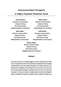
Figure 4. 3DBug in env3, as the robot moves into the room. (a) The entire path of 3DBug, compared to the globally optimal path. (b) The blocking contour computed from S, shown in bold line. (c) The blocking contour from F I . (d) The blocking contour from F2. The target is directly visible from F3.

167

T (invisible)

Figure 5 . 3DBug in env4. (a,b) The robot leaves house1 from the window, and enters house2 from the door. The globally optimal path is almost identical to 3DBug’s path. (c) The blocking contour from S. (d) The blocking contour from FI (located at the internal window frame).

3DBug’s paths in e m 2 is 1.02. In both envl and env2 the algorithm used the motion-towards-the-target mode along the entire path in over 99% of the runs. The environment env3 consists of a single concave room-like obstacle (Fig. 4 ) . The average path length in this environment is 1.06 (relative to the generalized visibility graph shortest path), and the surface-traversing mode was activated in 65% of the runs. The last environment env4 consists of two room-like obstacles, separated by a wall (Fig. 5). The start and target points were always placed inside or near the rooms, on different sides of the separating wall. In this environment the average path length of 3DBug is 1.03. The tested scenarios constitute only a preliminary study. There are other environments, in which the locally optimal decisions do not necessarily lead to globally optimal paths, and in these environments 3Dbug would be less effective. The local characteristics of 3DBug: The paths of 3DBug are distinct from the globally optimal ones for several reasons. As demonstrated in Figure 4 , the locally shortest path may differ from the globally optimal one due to the limited nature of local information. From S, the robot moves towards the ”roof” of the room, since the roof is not visible from S and thus considered non-existent (Fig. 4 ( b ) ) . After observing

the roof from FI, the robot moves along the shortest path from Fl to T . Partial occlusion is another manifestation of the limited nature of local information, as demonstrated in Figure 3. Using the motion-towardsthe-target mode, the robot moves from S to the focus point Fl, which lies on an occluding edge (Fig. 3(a)). The robot chooses this path from S since it does not see the entire blocking obstacle, denoted 01, and occluded portions of obstacles are considered as non-existent. Another reason for the difference between the two paths is the incorporation of the global convergence requirement during motion-towards-the-target. Restricting the computed shortest path to the feasible sub-contour may prevent the robot from moving along the precise locally shortest path, which may pass through any point on the blocking contour. Thus there are several reasons which cause 3DBug’s paths to differ from the globally optimal ones. 3DBug as a search algorithm: Last we discuss the search characteristics of 3DBug. In the graph-search terminology, the motion-towards-the-target mode is a hill-descending strategy, and the surface-traversing mode is a mechanism for escaping local minima. For comparison, we consider the classical A* algorithm which uses the generalized visibility graph as the underlying search space. The 3DBug algorithm finds the target in fewer steps than A* for the following reasons. First, 3DBug performs a depth search, thus it moves faster towards the target. Second, the candidate locations for the next step in 3DBug are limited to a single obstacle, which is the blocking obstacle in both modes of motion. In contrast, A* must consider all the nodes which are visible from each node U in the generalized vis-

ibility graph. In env3, for example, 3DBug reaches the target after 3.3 steps on average, while A* requires 32.4 steps to reach the target. The advantage of 3DBug is even more pronounced when the target is unreachable. The 3DBug algorithm concludes target unreachability after exploring the entire surface of a single obstacle in which the target is trapped, while A* must expand all the nodes in its search space to conclude unreachability. Another advantage of 3DBug is that it uses a compact data structure, since it uses only a limited amount of global information. In contrast, a data structure which represents the entire environment may be very large. For example, the generalized visibility graph of env2 with resolution 0.1 consists of 620 nodes and 118912 edges, while 3DBug’s data structure consists on the average of 7 nodes and 9 edges. 5

Concluding Discussion

We presented new basic results in sensor-based surface exploration, and locally shortest path computation in three-dimensional polyhedral environments. Consider-

168

ing surface exploration, we showed that the entire surface of a polyhedral obstacle is visible from the convex obstacle edges within the obstacle’s convex hull. Then we introduced the notion of a locally shortest path in three-dimensions, and showed that it must pass through the blocking contour. We used this property to formulate an efficient technique for estimating the locally shortest path in time linear in the number of edges in the blocking contour. These results were incorporated into the new globally convergent 3 D B u g algorithm, which navigates a point robot equipped with position and range sensors in a three-dimensional unknown environment. The algorithm falls within the general framework of the Bug paradigm since it strives to process the sensory data in the most reactive way possible, without sacrificing the global convergence guarantee. During motion towards the target, the robot follows the locally shortest path in a purely reactive fashion. During traversal of an obstacle surface, the robot incrementally constructs the CEG of the obstacle, while performing local shortcuts based on the local range data. Simulation results show that 3 D B u g generates paths which resemble the globally shortest path in simple scenarios, consisting of disjoint convex obstacles. Moreover, the algorithm generates reasonably short paths even in concave, room-like environments. Let us mention several potential uses and extensions for the new algorithm. First, 3 D B u g is useful for navigating free-flying robots in either real tasks such as surveillance, or in simulated scenarios such as virtual reality games. Second, 3 D B u g provides new insight into the important problem of sensor-based navigation in three-dimensions. Third, the algorithm can be extended to other three-dimensional configuration spaces, such as the ones associated with three degrees-of-freedom mobile robots. Last, 3 D B u g is also useful as a search algorithm in completely known three-dimensional environments. The main advantage of 3Dug over classical search algorithms such as A* is that it takes into consideration the geometric characteristics of the locally shortest path. Consequently, 3 D B u g finds the target much faster than other, less informed, algorithms. References R. Chatila. Deliberation and reactivity in autonomous mobile robots. Robotics and Autonomous Systems, 16:197-211, 1995. G. Foux, M. Heymann, and A. Bruckstein. Two dimensional robot navigation among unknown stationary polygonal obstacles. IEEE Transactions on Robotics and Automation, 9(1):96-102, 1993.

169

I. Kamon, E. Rimon, and E. Rivlin. Tangentbug: A range-sensor based navigation algorithm. To appear in the International Journal on Robotic Research. I. Kamon, E. Rimon, and E. Rivlin. Range-sensor based navigation in three dimensions. CIS 9712, Center of Intelligent Systems, Dept. of Computer Science, Technion, Israel, 1997. K. N. Kutulakos, V. J. Lumelsky, and C. R. Dyer. Vision guided exploration: a step toward general motion planning in three dimensions. I E E E Conf. on Robotics and Automation, 289-296, 1993.

T. Lozano-Perez and M. A. Wesley. An algorithm for planning collision free paths among polyhedral obstacles. Communications of the A C M , 22(10):560-570, 1979. V. J. Lumelsky. A comparative study on the path length performance of maze-searching and robot motion planning algorithms. I E E E Transactions on on Robotics and Automation, 7(1):57-66, 1991. V. J. Lumelsky and A. A. Stepanov. Path-planning strategies for a point mobile automaton moving amidst obstacles of arbitrary shape. Algoritmica, 2:403-430, 1987. C. H. Papadimitriou. An algorithm for shortest path motion in three dimensions. Information processing letters, 20:259-263, 1985.

N. S. V. Rao and S. S. Iyengar. Autonomous robot navigation in unknown terrains: visibility graph based methods. I E E E transactions on Systems, Man and Cybernetics, 20(6):1443-1449, 1990.

J. H. Rieger. The geometry of view space of opaque objects bounded by smooth surfaces. Artificial Intelligence, 44:l-40, 1990.

A. Sankaranarayanan and M. Vidyasagar. Path planning for moving a point object amidst unknown obstacles in a plane: the universal lower bound on worst case path lengths and a classification of algorithms. I E E E Conf. on Robotics and Automation, 1734-1941,1991. A. Stentz. Optimal and efficient path planning for partially known environments. I E E E Conf. on Robotics and Automation, 3310-3317, 1994. C. J. Taylor and D. J. Kriegman. Vision based motion planning and exploration algorithms for mobile robots. Workshop on Algorithmic Foundations of Robotics, 69-83. A K Peters, 1995.