Feb 5, 2012 - We consider rank modulation codes for flash memories that allow for handling ... codes and arrays under a number of performance metrics.
arXiv:1202.0932v1 [cs.IT] 5 Feb 2012
Rank Modulation for Translocation Error Correction∗ Farzad Farnoud, Vitaly Skachek, and Olgica Milenkovic University of Illinois, Urbana-Champaign February 7, 2012
Abstract We consider rank modulation codes for flash memories that allow for handling arbitrary charge drop errors. Unlike classical rank modulation codes used for correcting errors that manifest themselves as swaps of two adjacently ranked elements, the proposed translocation rank codes account for more general forms of errors that arise in storage systems. Translocations represent a natural extension of the notion of adjacent transpositions and as such may be analyzed using related concepts in combinatorics and rank modulation coding. Our results include tight bounds on the capacity of translocation rank codes, construction techniques for asymptotically good codes, as well as simple decoding methods for one class of structured codes. As part of our exposition, we also highlight the close connections between the new code family and permutations with short common subsequences, deletion and insertion error-correcting codes for permutations and permutation arrays.
1
Introduction
Permutation codes and permutation arrays are collections of suitably chosen codewords from the symmetric group, used in applications as varied as single user communication over Gaussian channels [29, 20], reduction of impulsive noise over power-lines [4, 9], rank aggregation [21, 28, 23] and coding for storage [5]. Many instances of permutation-based codes were studied in the coding theory literature, with special emphasis on permutation arrays under the Hamming distance and rank modulation codes under the Kendall τ distance [22, 11, 6][12, Chapter 6B]. The distances used for code construction in storage devices have mostly focused around two families of combinatorial measures: adjacent and arbitrary transpositions and measures obtained via embeddings into the Hamming space [5, 4]. This is due to the fact that such distance measures capture the displacement of symbols in retrieved messages that arise in modern storage systems. One of the most prominent emerging applications of permutation codes in storage is rank modulation. Rank modulation is an encoding scheme for flash memories that may improve the lifespan, storage efficiency and reliability of future generations of these storage devices [18, 5, 31, 19]. The idea behind the modulation scheme is that information should be stored in the form of rankings of the cells charges, rather than in terms of the absolute values of the charges. This simple conceptual coding framework may reduce the problem of cell block erasures as well as potential cell over-injection issues [18, 34]. In their original formulation, rankmodulation codes represent a family of codes capable of handling errors of the form of adjacent transpositions. Such transposition errors represent the most likely errors in a system where the cells have nearly-uniform leakage rates. Leakage rates depend on the charge of the cells, the position of the cells but also on a number ∗ This work was supported by the NSF STC-CSoI 2011 and NSF CCF 0809895 grants and a AFRLDL-EBS AFOSR Complex Networks grant.
1
of external factors, the influence of which may not be adequately captured by adjacent transposition errors. For example, sudden and steep drops in the charge of one group of cells cannot be modeled in this framework. In what follows, we present a novel approach to rank modulation coding which allows for correcting a more varied class of errors when compared to classical schemes. The focal point of the study that follows is the notion of a translocation error, a concept that generalizes the notion of a transposition in a permutation. Roughly speaking, a translocation1 moves the ranking of one particular element in the permutation below the ranking of a certain number of closest-ranked elements. As such, translocations are suitable for modeling errors that arise in flash memory systems were sudden drops of cell charges or high leakage levels for subsets of cells are expected or possible. A translocation may be viewed as an extension of an adjacent transposition to a transposition of elements a certain number of locations apart. In addition, translocation correspond to pairs of deletions and insertions of an element in the permutation. As a consequence, the study of translocations is also closely related to a number of problems in combinatorial theory such as the longest common subsequence problem and permutation coding under the Levenshtein and Hamming metric [32, 17, 24]. The rank modulation problem is by now fairly well understood from the perspective of code construction. The capacity of rank-modulated channel was derived in [5, 26, 1], while some practical code constructions were proposed in [5, 18], and further generalized in [25], [15] and [26]. Here, we complement the described work in terms of deriving upper and lower bounds on the capacity of translocation rank modulation codes, and in terms of presenting constructive, asymptotically good coding schemes. Our constructions are based on a novel idea of permutation interleaving, and are of independent interest in combinatorics and algebra. Furthermore, we propose decoding algorithms for translocation codes based on decoders for codes in the Hamming metric [30, 33]. As part of our analysis, we describe the close relationships between permutation codes and arrays under a number of performance metrics. The paper is organized as follows. In Section 2 we provide the motivation for studying translocations as well as basic definitions used in our analysis. The properties of permutations under translocations are studied in the same section while bounds on the size of the codes are presented in 3. Code constructions are presented in Sections 4 and Section 5, while concluding results are presented in Section 6.
2
Basic definitions
Throughout the paper, we use the following notation. The set of nonnegative integers is denoted by Z+0 , while [n] ∶= {1, 2, ⋯, n} stands for the set of non-negative integers not exceeding n.
A permutation is a bijection σ ∶ [n] → [n], that is, for any i, j ∈ [n], i ≠ j, we have σ(i) ≠ σ(j). For any σ ∈ Sn , we write σ = (σ(1), σ(2), ⋯, σ(n)), where σ(i) is the image of i ∈ [n] under the permutation σ. Alternatively, we may write σ as [σ(1), σ(2), ⋯, σ(n)] or as [σ(1)σ(2)⋯σ(n)] if doing so does not cause ambiguity. The identity permutation (1, 2, ⋯, n) is denoted by e, while σ −1 stands for the inverse of the permutation σ. Permutations are denoted by Greek lowercase letters, while integers and integer vectors are denoted by Latin lower case symbols. We let Sn denote the set of all permutations of the set [n], i.e., the symmetric group of order n. Additionally, let S (P ) , P ⊆ [n], be defined as the set of all permutations of elements of P . A permutation code of length n and minimum distance d in a metric d is subset C of Sn such that for all distinct π, σ ∈ C, we have d(π, σ) ≥ d. 1 Note that our definition of the term translocation differs from a definition of this term commonly used in biology. See, e.g., [35].
2
6
3
6 8
1 2
4
9
Leakage
8
3
1
5
5
9
2 4
7
7
[683159247]
[638159247]
Figure 1: Rank modulation codes and adjacent transposition errors. Definition 1. We say that a permutation τ ∈ Sn is a transposition if for i, j ∈ [n], τ = (1, ⋯, i − 1, j, i + 1, ⋯, j, i, j + 1, ⋯, n).
If j = i + 1, then τ is called an adjacent transposition. Assume that 1 ≤ i, j ≤ n. A translocation φ(i, j) is a permutation defined as follows. If i ≤ j, we have φ(i, j) = (1, ⋯, i − 1, i + 1, i + 2, ⋯, j, i, j + 1, ⋯, n) and if i > j, we have
φ(i, j) = (1, ⋯, j − 1, i, j, j + 1, ⋯, i − 1, i + 1, ⋯, n) .
For i ≤ j, the permutation φ(i, j) is called a right translocation and the permutation φ(j, i) is called a left translocation. Example 2. Assuming i ≤ j, for σ = (σ(1), ⋯, σ(n)), we have
στ = (σ(1), ⋯, σ(i − 1), σ(j), σ(i + 1), ⋯, σ(j − 1), σ(i), σ(j + 1), ⋯, σ(n)).
and
σφ(i, j) = (σ(1), σ(2), ⋯, σ(i − 1), σ(i + 1), σ(i + 2), ⋯, σ(j), σ(i), σ(j + 1), ⋯, σ(n)) .
σφ(j, i) = (σ(1), σ(2), ⋯, σ(i − 1), σ(j), σ(i), σ(i + 1), ⋯, σ(j − 1), σ(j + 1), ⋯, σ(n)) .
In particular, let σ = (1, 3, 5, 7, 2, 4, 6, 8). For this case, σφ(3, 6) = (1, 3, 7, 2, 4, 5, 6, 8)
and
σφ(5, 2) = (1, 2, 3, 5, 7, 4, 6, 8) .
Simply put, the product of the permutation σ and a translocation φ(i, j) is the permutation obtained by moving σ(i) to the j-th position and shifting all the elements between the i-th and j-th positions. Observe that the inverse of the left translocation φ(i, j) is the right translocation φ(j, i), and vice versa. Our interest in translocations in permutations is motivated by rank modulation coding, as illustrated by the examples depicted in Figures 1 and 2. In classical multi-level flash memories, each cell used for storing information is subjected to errors. As a result, classical error control schemes of non-zero rate can not be efficiently used in such systems. One solution to the problem is to encode the information in terms of rankings [22], rather than absolute values of the stored information sequences. As a result, data is represented by permutations and errors manifest themselves via reordering of the ordered elements. The simplest model 3
6
3
6 8
1
5 2
4
8
1 5
9
Leakage
3
7
[638159247]
9
2 4
7
[681592437]
Figure 2: Rank modulation codes and translocation errors caused by “large” drops of charge levels.
assumes that only adjacent ranks may be exchanged – or equivalently, that only adjacent positions in the inverse permutation may be exchanged. This model has the drawback that it does not account for more general changes in ranks. With respect to this observation, consider the charge-drop model in Figure 2. Here, cell number 3, ranked second, experienced a leakage rate sufficiently high to move the cells ranking to the seventh position. If other cells had significantly more moderate leakage rates, the resulting ranking would be the result of a (right) translocation error. It is easy to note that in this framework, one translocation φ(i, j) of “length” ∣i − j∣ corresponds to ∣i − j∣ adjacent transpositions. Nevertheless, a translocation should be counted as a single error, and not a sequence of adjacent transposition errors. The translocation error model may appear to be too broad to describe the phenomena arising in flash memories, as error models corresponding to translocations of small length arise more frequently than translocations of long length. The idea of bounded length translocations will be pursuit further in a companion paper. We only remark that translocation errors of arbitrary length are of interest since they are suitable for accounting for arbitrary charge drops of any cell independently of the drops of other cells. This makes them a good candidate for studying new error-control schemes in flash memories. We formalize the notion of translocation distance below. Definition 3. Let σ, π ∈ Sn . The translocation distance between σ and π is a function d○ (σ, π) ∶ Sn × Sn → Z+0 , defined as the minimum number of translocations needed to transform σ to π. In other words, d○ (σ, π) equals the smallest m such that there exist a sequence of translocations φ1 , φ2 , ..., φm for which π = σφ1 φ2 ⋯φm . Observe that the function d○ (⋅, ⋅) is nonnegative and symmetric. It also satisfies the triangle inequality, namely for any σ1 , σ2 and σ3 in Sn , one has d○ (σ1 , σ3 ) ≤ d○ (σ1 , σ2 ) + d○ (σ2 , σ3 ) . Therefore, it is indeed a metric over the space Sn . Note that a translocation may correspond to either a left or a right translocation. As seen from the example in Figure 2, right translocations correspond to general cell leakage models. On the other hand, left translocation assume that the charge of a cell is increased above the level of other cells, which corresponds to a phenomena not frequently encountered in flash memories. We therefore also introduce the notion of the 4
right translocation distance. As will be seen from our subsequent discussion, the translocation distance is much easier to analyze than the right translocation distance, and represents a natural lower bound for this distance. Definition 4. A subsequence of length m of σ = (σ(1), . . . , σ(n)) is a sequence of the form σ(i1 ), . . . , σ(im ), with i1 < i2 < . . . im . Let σ1 , σ2 ∈ Sn . The longest common subsequence of σ1 and σ2 is a subsequence of both σ1 and σ2 of longest length. We denote this sequence by L (σ1 , σ2 ), and its length by l (σ1 , σ2 ).
Definition 5. Let σ ∈ Sn and let l (σ) ∶= l (σ, e). The function l (σ) is termed the length of the longest increasing subsequence of σ. Definition 6. Let R+0 denote the set of nonnegative real numbers. A metric d ∶ Sn × Sn → R+0 is rightinvariant if, for all π, σ, ω ∈ Sn , we have d(π, σ) = d(πω, σω). Similarly, d is left-invariant if d(π, σ) = d(ωπ, ωπ).
Intuitively, a right-invariant metric is invariant with respect to reordering of elements and a left-invariant metric is invariant with respect to relabeling of elements. Furthermore, if d(π, σ) is a right-invariant metric, then it is applied to π(i) and σ(i) and if it is a left-invariant metric, it is applied to π −1 (i) and σ −1 (i). It can be easily verified that the translocation distance is a left-invariant metric. The length of the longest common subsequence is also easily seen to be left-invariant. Proposition 7. For π, σ ∈ Sn , the distance d○ (π, σ) equals n − l (π, σ). Proof. By the left-invariance of d○ and l, we may assume that one of the permutations is the identity permutation e since otherwise, instead of d○ (π, σ) = n − l (π, σ), we can show that d○ (σ −1 π, e) = n − l (σ −1 π). It thus suffices to prove that d○ (σ, e) = n − l (σ). Let Sℓ denote the set of elements in the longest increasing subsequence of the permutation σ. Clearly, it is possible to transform σ to e with at most n − l(σ) translocations. This can be achieved by applying translocation that move one element from the set [n]/Sℓ to its position in the identity permutation e. Hence, d○ (σ, e) ≤ n − l (σ). Next, we show that d○ (σ, e) ≥ n − l (σ). We start with σ and transform it to e by applying a sequence of translocation. Every translocation increases the length of the longest increasing subsequence by at most one. Hence, we need at least n − l (σ) translocation to transform σ into e and thus, d○ (σ, e) ≥ n − l (σ).
Since the translocation distance between two permutations is a function of the length of their longest common subsequence, there exists an interesting connection between the translocation distance and Levenshtein’s edit distance for permutations [24]. The latter distance is used for measuring the influence of deletions and insertions on the “similarity” of two permutations. Formally, it may be defined as follows. Let the number of deletions and insertions required to transform u into v be denoted by ρ (u, v). Levenshtein [24] showed that, for sequences of length n over [n], ρ (u, v) = 2 (n − l(u, v)) . This equality also holds for permutations over Sn and thus ρ (σ1 , σ2 ) = 2d○ (σ1 , σ2 ) . This result may be also deduced directly, by observing that a translocation φ(i, j) in a permutation σ deletes the element σi and inserts the same element in location j.
It is also of interest to see how the translocation distance compares to the Kendall’s τ distance used for classical rank modulation coding. The Kendall’s τ distance dτ (σ, π) from σ ∈ Sn to π ∈ Sn is defined as the minimum number of adjacent transpositions required to change σ into π. A distance measure related to the Kendall’s τ distance is the transposition distance, dT (π, σ). The transposition distance between two permutations π and σ equals the smallest number of transpositions (not necessarily adjacent) needed 5
to transform π into σ. The transposition distance dT (π, σ), as shown by Cayley in the 1860s, equals the number of cycles in the permutation σ π −1 . Since a translocation of length ℓ requires at most ℓ − 1 adjacent transpositions, and since an adjacent transposition is a translocation, it is easy to see that 1 dτ (σ, π) ≤ d○ (σ, π) ≤ dτ (σ, π). n−1 Both the upper and lower bound are tight: the upper bound is achieved for π obtained from σ via a single adjacent transposition, while the lower bound is achieved for, say, σ = e and π = (2, 3, . . . , n, 1). It is also straightforward to show that the diameter of the translocation distance equals n − 1. Observe that the above inequalities imply that the translocation distance is not within a constant factor from the Kendall’s τ distance, so that code constructions and bounds specifically designed for the latter distance measure are not tight and sufficiently efficient with respect to the translocation distance. A similar pair of bounds may be shown to hold for the translocation distance and the Hamming distance between two permutations. The Hamming distance between two permutations σ, π, dH (σ, π) is defined as n − ∣F (σ, π)∣, where F (σ, π) denotes the set of fixed points in σ under the ordering of π (and vice versa).
The subsequence of σ consisting of elements of F (σ, π) is also a subsequence of π and thus d○ (σ, π) = n − l(σ, π) ≤ n − ∣F (σ, π)∣ = dH (σ, π). Furthermore, since for any two permutations π, σ ∈ Sn one has dH (π, σ) ≤ n, it follows that dH (π, σ) ≤ nd○ (π, σ). Thus, 1 dH (π, σ) ≤ d○ (π, σ) ≤ dH (π, σ) . n
(1)
These inequalities are sharp. For the upper-bound, consider π = [12⋯n] and σ = [n⋯21], with n odd. For the lower-bound, let π = [12⋯n] and σ = [23⋯n1] so that dH (π, σ) = n and d○ (π, σ) = 1. Next, we consider the Cayley metric. Note that each transposition may be viewed as two translocations, 1 implying d○ (π, σ) ≤ 2dT (σ, π). It is also immediate that n−1 dT (π, σ) ≤ d○ (π, σ). Hence, we have 1 dT (π, σ) ≤ d○ (π, σ) ≤ 2dT (σ, π). n−1 The relationship between the Hamming distance and Cayley’s distance can be explained as follows. When transforming π to σ using transpositions, each transposition decreases the Hamming distance between the two permutations by at most two. Hence, dT (π, σ) ≥ dH (π, σ)/2. Sorting a permutation of length d requires at most d − 1 transpositions. Thus, dT (π, σ) ≤ dH (π, σ) − 1. These inequalities result in 1 dH (π, σ) ≤ dT (π, σ) ≤ dH (π, σ) − 1. 2
(2)
There exist many embedding methods for permutations, allowing one set of permutations with desirable properties according to a given distance to be mapped into another set of permutations with good properties in another metric space [3]. In subsequent section, we exhibit a method for embedding permutations with good Hamming distance into the space of permutations with large minimum translocation distance.
2.1
Asymmetric translocation distance
We describe next how to specialize the translocation distance for the case that only right-translocations are allowed to occur. 6
Definition 8. Let π, σ ∈ Sn and denote by Rt (π, σ) the minimum number of right translocation required ⃗○ (π1 , π2 ) is defined to transform π into σ. For two permutations π1 , π2 ∈ Sn , the right translocation distance d as ⃗○ (π1 , π2 ) = 2 min {max {Rt (π1 , σ), Rt (π2 , σ)}} . d σ
⃗○ (π1 , π2 ) ≤ 2t if and only The definition implies that for two permutations π1 ∈ Sn and π2 ∈ Sn , one has d if there exists a permutation σ ∈ Sn such that Rt (π1 , σ) ≤ t and Rt (π2 , σ) ≤ t. Hence, a code C is t-right ⃗○ (π1 , π2 ) > 2t for all π1 , π2 ∈ C, π1 ≠ π2 . This means that under translocation correcting if and only if d the given distance constraint, it is not possible to confuse the actual codeword π1 with another (wrong) codeword π2 . Observe that the following bound holds: ⃗○ (π1 , π2 ) . d○ (π1 , π2 ) ≤ d It is straightforward to characterize the minimum number of right translocations needed to transform one permutation to another, as we show below. Definition 9. Let π, σ ∈ Sn . We denote the set of π −1 -increasing and σ −1 -decreasing elements as J (π, σ) ∶= {i ∈ [n] ∶ ∃j s.t. π −1 (i) < π −1 (j) and σ −1 (i) > σ −1 (j)} . Lemma 10. Let π, σ ∈ Sn . Then
Rt (π, σ) = ∣J (π, σ)∣ .
Proof. It can be easily verified that Rt is left-invariant. So it suffices to show that Rt (π, e) = ∣J (π, e)∣ , where
∣J (π, e)∣ = ∣{i ∈ [n] ∶ ∃j < i, π −1 (i) < π −1 (j)}∣ .
Let π1 be obtained from π by applying a right translocation. Then, it is straightforward to see that ∣J(π1 , e)∣ ≥ ∣J(π, e)∣ − 1. Thus, Rt (π, e) ≥ ∣J (π, e)∣ − ∣J (e, e)∣ = ∣J (π, e)∣.
Conversely, to transform π into e, it suffices to apply the shortest right translocation to each i ∈ J that moves i to position i′ such that to the left of positions i′ there are only elements smaller than i. Hence, Rt (π, e) ≤ ∣J (π, e)∣ .
For permutations π, σ ∈ Sn , the difference between Rt (π, σ) and d○ (π, σ) may be as large as n − 2. This may be seen by letting π = [23 . . . n1] and σ = e, and observing that Rt (π, σ) = n − 1 and d○ (π, σ) = 1. Furthermore, it can be shown that this is the largest possible gap. To see this, first, note that Rt (π, σ) = 0 if and only if d○ (π, σ) = 0 and thus to obtain a positive gap one must have d○ (π, σ) ≥ 1. We also have d○ (π, σ) ≤ Rt (π, σ) ≤ n − 1. Hence, 1 ≤ d○ (π, σ) ≤ Rt (π, σ) ≤ n − 1, which implies that the gap is at most n − 1 − 1 = n − 2. In the sections to follow, we focus our attention on the symmetric translocation distance. For simplicity, we omit the word symmetric.
7
3
Bounds on the size of the code
3.1
Codes in translocation distance
Let A○ (n, d) be the maximum size of a code of length n and minimum translocation distance d. Let denote the rate of the code. C○ (n) ∶= ln Aln○ (n,d) n! Proposition 11. For all integers n and d with n ≥ d ≥ 1, A○ (n, d) ≥
(n − d + 1)! ⋅ n (d−1 )
Proof. Let B○ (r) be the number of permutations with translocation distance at most r from a given permutation. By symmetry, we have B○ (r) = {σ ∶ d○ (π, e) ≤ r}. The permutations that are within distance r of π are precisely the permutations σ with l (π, σ) ≥ n − r. There are (nr) ways to choose the first n − r elements n! ways to arrange the remaining elements. of the longest common subsequence of π and σ and at most (n−r)! Hence, n n! B○ (r) ≤ ( ) ⋅ r (n − r)! From the Gilbert-Varshamov bound, we have A○ (n, d) ≥ A○ (n, d) ≥
n! B○ (d−1)
and thus
n!
n n! (d−1 ) (n−d+1)!
which completes the proof. Proposition 12. For all n, d ∈ Z with n ≥ d ≥ 1, A○ (n, d) ≤ (n − d + 1)! . Proof. We provide two proofs for this bound. The first proof is based on a projection argument first described in [1], while the second is based on a standard counting arguments associated with the proof of Plotkin’s bound2 . For σ ∈ Sn and P ⊆ [n], the projection σP of σ onto P is obtained from σ by only keeping elements of P and removing the other elements. For example, let σ = [54321], and P = {2, 4, 5}. We have σP = [542]. Note that σP has length ∣P ∣. 1) Let C be a code of length n, size M , and minimum distance d. Let k be the smallest integer such that σ{1,...,k+1} ≠ π{1,...,k+1} for all distinct σ, π ∈ C. Hence, M ≤ (k + 1)!. By definition, there exist σ, π ∈ C such that σ{1,...,k} = π{1,...,k} . So, l (σ1 , σ2 ) ≥ k and thus d ≤ d○ (σ1 , σ2 ) ≤ n − k. Hence, M ≤ (n − d + 1)!. 2) Again, let C be a code of length n, size M , and minimum distance d. Since the minimum distance n n! ) subsequences of length n − d + 1 of codewords of C are unique. There are (d−1)! is d, all M (n−d+1 possible subsequences of length n − d + 1. Hence, M( which implies that M ≤ (n − d + 1)!. 2
n n! )≤ (d − 1)! n−d+1
The authors gratefully acknowledge a number of discussions with Jalal Etesami.
8
From the two previous propositions, we obtain (n − d + 1)! ≤ A○ (n, d) ≤ (n − d + 1)! n (d−1 )
(3)
All limits that appear in the rest of the paper are in n unless otherwise stated. The results below are stated for code families with length n, M (n) codewords, and minimum translocation distance d(n). The ratio d(n)/n is denoted by δ(n). Furthermore, lim δ(n) and lim C○ (n) are denoted by δ and C○ respectively. Lemma 13. We have that
1. lim
ln(n − d(n))! = 1 − δ, ln n!
2. lim
n! ln d(n)!
3. lim Proof.
ln n!
= 1 − δ,
n ) ln (d(n)
ln n!
= 0.
1. ln (n − d(n))! (n − d(n)) ln (n − d(n)) + O (n) = ln n! n ln n + O (n) n ln n − d(n) ln n + (n − d(n)) ln (1 − d(n)/n) + O (n) = n ln n + O (n) 1 d(n) +O( ) =1− n ln n
2. n! ln d(n)!
ln n!
ln n! − ln d(n)! ln n! d(n) ln d + O (n) =1− n ln n + O (n) 1 d(n) ln d(n) +O( ) =1− n ln n ln n d(n) ln n + d(n) ln (d(n)/n) 1 =1− +O( ) n ln n ln n 1 d(n) +O( ) =1− n ln n =
3. From parts 1 and 2, it follows that n ) ln (d(n)
ln n!
=
n! − ln (n − d(n))! ln d(n)!
ln n!
9
= O(
1 ) ln n
The following theorem provides expressions for the asymptotic capacity of the translocation channel. Theorem 14. Let C be a family of translocation correcting codes of length n, distance d(n). Then C○ = 1 − δ. Proof. From (3), we have n ) ln (n − d + 1)! − ln (d−1
ln n!
≤ C○ (n) ≤
ln (n − d + 1)! ln n!
(4)
Taking the limit of (4) by using Lemma 13 yields C○ = lim C○ (n) = 1 − lim δ(n) = 1 − δ.
(5)
At this point, it is worth observing that the problem of bounding the longest common subsequence in permutations has been recently studied in a combinatorial framework in [2]. In this framework, the question of interest is to determine the minimum length of the longest common subsequence between any two distinct permutations in a set of k permutations of length n. When translated into the terminology of translocation coding, the problem reduces to finding dk (n), the largest possible minimum translocation distance of a set of k permutations of Sn . The bounds derived in [2] are constructive, but they hold only in the zero-capacity domain of parameters. A more detailed description of this construction is described in the next section. The bounds of [2] imply √ √ 1/3 1/3 that dk (n) ≥ n − 32 (nk) for 3 ≤ k ≤ n. Hence, for n − 32 n ≤ d ≤ n − 32 (3n) , A○ (n, d) ≥
Furthermore, for k ≥ 4, dk (n) ≥ n − ⌈n1/(k−1) ⌉
k/2−1
1 n−d 3 ( ) . n 32
. For k ≥ 2 (1 + log2 n), this bound is of no practical use.
For 1 + log2 n ≤ k < 2 (1 + log2 n), one has dk (n) ≥ n − 2k/2−1 which implies that,
A○ (n, d) ≥ 2 (1 + log2 (n − d)) √ 1 for d ≤ n − n/2. Similar bounds can be obtained for A○ (n, d) by assuming that m − 1 < n k−1 ≤ m for some integer m ≤ ⌈n1/3 ⌉. Note that although these results hold for the zero-capacity regime, they still may be useful for finite codelength. Remark: Similar bounds may be derived for asymmetric translocation error-correcting codes. For this ⃗ purpose, let B ′ (r) = ∣{σ ∶ Rt (e, σ) ≤ r}∣ and B(r) = ∣{σ ∶ ⃗ d○ (e, σ) ≤ r}∣. Then n! n! n! ≤ ≤ A⃗ (n, 2t) ≤ ′ ⃗ B○ (2t) B(2t) B (t)
⃗ d) denotes the maximum size of a permutation code with minimum right-translocation distance where A(n, d.
3.2
Relationships among codes with translocation, substitution, deletion/insertion and transposition errors
Translocation errors, and consequently, translocation error correcting codes are difficult to analyze directly. As already pointed out, the translocation distance is related to various other metrics well-studied in the 10
coding theory and mathematics literature. Since the constructions in subsequent sections rely on code constructions for other distance metrics, we provide a brief overview of the state of the art results pertaining to the Hamming, transposition and Kendall τ metric. We also supplement the known findings with a number of new comparative results for the metrics of interest. 3.2.1
Hamming metric
Codes in the Hamming metric have a long history, dating back to the work [13]. The Hamming metric is a suitable distance measure for use in power line communication systems, database management and other applications. Let AH (n, d) denote the largest number of permutations of length n and Hamming distance d. Frankl and Deza [13, Theorem 4] and Deza [10] showed that n! n! ≤ AH (n, d) ≤ BH (d − 1) (d − 1)!
where BH (r) is the volume of the sphere of radius r in the space of permutations with Hamming metric. Let Di denote the number of derrangments of i objects, i.e., the number of permutation of i objects at Hamming distance i from the identity permutation. It can be shown that BH (r) = 1 + ∑ri=2 (ni)Di . Hence, d−1 d−1 n n! BH (d − 1) = 1 + ∑ ( )Di ≤ ∑ (n − i)! i i=2 i=1 n! ≤ (d − 1) (n − d + 1)!
where the first inequality follows from the fact that Di ≤ i!. Note that although a more precise asymptotic characterization for the number of derrangements is known, namely Dℓ 1 = ,, ℓ→∞ ℓ! e lim
the simple bound Di ≤ i! provides sufficiently tight bound for the capacity computation. The above results show that
n! (n − d + 1)! ≤ AH (n, d) ≤ d−1 (d − 1)!
Lemma 13 implies the following theorem. As before, the result holds for a family of codes C under the Hamming distance metric, with parameters n, d and δ(n). Theorem 15. If δ(n) = d(n)/n denotes the normalized Hamming distance, then the capacity of the Hamming permutation channel equals CH = 1 − lim δ(n). 3.2.2
Transposition metric
Let AT (n, d) denote the maximum size of a code with minimum transposition distance dT at least d. From (2), we have AH (n, 2d) ≤ AT (n, d) ≤ AH (n, d − 1) . The upper-bound and a sharper lower bound may also be derived from the following proposition.
11
Proposition 16. For all n and d, n!
n−i n ∑i=n−d+1 (−1) s (n, i)
where s (n, k) is the Stirling number of the first kind.
≤ AT (n, d) ≤
n! d!
Proof. Let C be the largest possible code of length n with minimum transposition distance d, and with M codewords. Furthermore, let γm ∶ Sn → Sm be a mapping such that γm (σ) = (σ (1) , σ (2) , . . . , σ (m)). Let k be the smallest integer such that γk+1 is injective when applied to C. Then, we have M ≤ n (n − 1) ⋯ (n − k) = n! . Since, γk is not injective, there exist permutations σ1 , σ2 ∈ C such that γk (σ1 ) = γk (σ2 ). Hence, (n−k−1)! d ≤ dT (σ1 , σ2 ) ≤ n − k − 1 and thus M ≤
n! . d!
To prove the lower bound, note that AT (n, d) ≥
n! BT (d − 1)
where BT (r) is the size the ball {π ∶ dT (π, e) ≤ r}. It is well-known that dT (π, e) = n − c (π), where c (π) n−k denotes the number of cycles of π, and that the number of permutations with k cycles equals (−1) s (n, k). n−i Hence, {π ∶ dT (π, e) ≤ d − 1} = {π ∶ c (π) ≥ n − d + 1} and consequently BT (d − 1) = ∑ni=n−d+1 (−1) s (n, i). Using the bounds above, we have the following theorem. Theorem 17. The capacity CT of the transposition channel is bounded as 1 − 2 lim δ(n) ≤ CT ≤ 1 − lim δ(n). 3.2.3
Kendall’s τ metric
Let AK (n, d) denote the largest cardinality of a permutation code of length n with minimum Kendal’s tau distance d, and let CK = lim ln AK (n,d)/ln n!. Barg and Mazumdar [1, Theorem 3.1] showed that CK = 1 − ǫ,
for d = Θ (n1+ǫ ) .
Note that for the Kendall τ metric, the maximum distance between two permutations may be as large as O(n2 ). On the other hand, the diameter of the translocation distance is O(n). 3.2.4
Levenshtein metric
The bounds on the size of deletion/insertion correcting codes over permutations were first derived by Levenshtein in his landmark paper [24]. The lower bound relies on the use of Steiner triple systems and designs [24]. More precisely, let D(n, q) be the largest cardinality of a set of n-subsets of the set {0, 1, . . . , q − 1} with the property that every (n − 1)-subset of {0, 1, . . . , q − 1} is a subset of at most one of the n-subsets. Then the following results holds for the cardinality AL (n, q) of the largest single-deletion correcting codes over permutations in Sq [24]: q! (n − 1)!D(n, q) ≤ AL (n, q) ≤ . n (q − n + 1)! For a more thorough discussion regarding perfect permutation codes in the Levenshtein metric over Sq , capable of correcting n − t errors and ordered Steiner systems S(t, q, q), the interested reader is referred to [24]. 12
4
Single error correcting codes for translocations and right-translocations
This section contains constructions for single-translocation error detecting and single-translocation error correcting codes. For the latter case, we exhibit two constructions, one for symmetric translocations and another for right-translocations only. The constructions are based on codes in the Levenshtein and Hamming metric. We start by describing how to construct single-translocation detecting codes based on single-deletion correcting codes for permutations. From the discussion in Section 2, recall that the translocation distance is half of the deletion distance and thus any single-deletion correcting code may be used for detecting a single translocation. An elegant construction for single-deletion correcting codes for permutation was described by Levenstein in [24]. The resulting code has cardinality (n − 1)! and is optimal, since, from Proposition 12, we have A○ (n, 2) ≤ (n − 2 + 1)! = (n − 1)!.
Hence, A○ (n, 2) = (n − 1)!.
Levenstein’s construction is of the following form. For a ∈ {0, 1, ⋯, n}, let
n
W2n = {u ∈ {0, 1} ∶ (n + 1) ∣ ∑ iu (i)} n
i=1
where a ∣ b denotes that a is a divisor of b. For σ ∈ Sn , let Z (σ) = (z (1) , ⋯, z (n − 1)) be a vector with ⎧ ⎪ ⎪0, z (i) = ⎨ ⎪ ⎪ ⎩1,
Levenstein shows that the code
if σ (i) ≤ σ (i + 1) , if σ (i) > σ (i + 1) ,
C = {σ ∈ Sn ∶ Z (σ) ∈ W2n−1 } ,
i ∈ [n − 1] . (6)
of size (n − 1)! is capable of correcting a single deletion. Hence, this code can detect a single translocation error as well. Let Sn (t) be the set of permutations σ of length n−t that can be obtained from some ω ∈ Sn by t deletions. In other words, Sn (t) is the set of words of length n − t from the alphabet [n], without repetitions. A code C ⊆ Sn is a perfect code capable of correcting t deletions if, for every σ ∈ Sn (t) , there exists a unique π ∈ C such that σ can be obtained from π by t deletions. n ) (n − t)! and It was shown in [24] that C in (6) is a perfect code. Since the size of Sn (t) equals (n−t n (t) ( t ) elements of Sn can be obtained by t deletions from each σ ∈ C, we have that ∣C∣ = (n − t)!. Thus a perfect code capable of correcting t deletions, if it exists, is a code with minumum translocation distance t + 1. Hence, if such a code exists, it is an optimal code for translocation errors.
Next, we describe codes capable of correcting a single translocation error and codes capable of correcting a single right translocation error. The sizes of these two codes are identical, although the latter family of codes has a 1.5 higher rate. In the construction, we make use of a single-transposition error detecting code, described below. A single-transposition error detecting code: For σ1 , σ2 ∈ Sn , let dT (σ1 , σ2 ) as before denote the transposition distance between σ1 and σ2 . The parity of a transposition σ is defined as the parity of dT (σ, e). 13
It is well-known that applying a transposition to a permutation changes the parity of the permutation, and also that, for n ≥ 2, half of the permutations in Sn are even and half are odd 3 . Hence, the code C containing all even permutations of Sn is a single-transposition error detecting code of length n and cardinality Sn /2.
4.1
Right-translocation errors
In this subsection, we present a construction for codes that correct a single right-translocation error. For this purpose, we first define the operation of interleaving vectors (permutations) and codes. Definition 18. For permutations or projections of permutations σi , i ∈ [k], of lengths mi with m ≤ mk ≤ ⋯ ≤ m1 ≤ m + 1, the interleaved vector is defined as σ = σ1 ○ σ2 ○ ⋯ ○ σk , consisting of elements σ(j) = σi (⌈j/k⌉),
where i ≡ j (mod k). For a class of k codes Ci , let
k
1 ≤ j ≤ ∑ mi
(7)
i=1
C1 ○ ⋯ ○ Ck = {σ1 ○ ⋯ ○ σk ∶ σi ∈ Ci , i ∈ [k]}.
(8)
σ ○ π = (σ(1), π(1), σ(2), π(2), ⋯, σ(m), π(m))
(9)
σ ○ π = (σ(1), π(1), σ(2), π(2), ⋯, σ(m)).
(10)
For example, for vectors σ and π of length m, we have
and for vectors σ and π of lengths m and m − 1 respectively, we have
To construct a code capable of correcting a single right-translocation, we partition [n] into two sets, P0 and P1 , of sizes ⌊n/2⌋ and ⌈n/2⌉, respectively. Let Ci be the set of even permutations of elements of Pi , for i = 0, 1. Proposition 19. The interleaved code C0 ○ C1 corrects a single right-translocation error. Proof. Suppose n is even. The proof for odd n is similar. Furthermore, suppose that P0 and P1 consist of even and odd numbers in [n], respectively. Given the permutation ω, we want to find the unique π such that ω = πφ(i, j), i ≤ j. The kth element of ω is out of place if k ≡/ ω (k) (mod 2). It is easy to see that i = kmin ∶= min {k ∶ k ≡/ ω (k) (mod 2)} ,
i.e., i equals the smallest k such that the kth element of ω is out of place. Finding j is slightly more complicated since we must consider two different cases. Let kmax ∶= max {k ∶ k ≡/ ω (k) (mod 2)}. First, suppose that j ≡ i (mod 2). One can see that, in this case, j = 1 + kmax . Second, suppose that j ≡/ i (mod 2). Then, we have j = kmax . Hence, j ∈ {kmax , kmax + 1}. This ambiguity comes from the fact that ω (kmax ) and ω (1 + kmax ) have the same parity.
Let π0 ∶= ωφ(kmax , 1) and π1 ∶= ωφ(1 + kmax , 1). Furthermore, let σh , for l ∈ {0, 1} and h ∈ {0, 1}, be the subcode of πl consisting of elements of Ph . In words, π0 gives rise to the two component codewords (0) (0) (0) (0) σ0 and σ1 , where σ0 consists of even numbers and σ1 consists of odd numbers. Similarly, π1 gives (1) (1) rise to two component codewords σ0 and σ1 with the same properties as described for π0 . It can be (1) (0) (1) (0) (1) (0) easily verified that σ0 = σ0 and that σ1 = σ1 (ω (kmax ) ω (1 + kmax )). That is, σ1 and σ1 differ only in the transposition of elements ω (kmax ) and ω (1 + kmax ). Since the underlying subcode is a single (1) (0) transposition-error detecting code, only one of the σ1 and σ1 is valid. Thus, π is unique. (l)
3
More precisely, the symmetric group can be partitioned into the alternating group and its coset.
14
The cardinality of the interleaved code C0 ○ C1 equals ln (1/4) + 2 ln ⌊ n2 ⌋! ln n!
4.2
∼
1 4
⌈ n2 ⌉! ⌊ n2 ⌋!, and its rate asymptotically equals
n ln n + O (n) ∼ 1. n ln n + O (n)
Translocation errors
The following construction leads to single translocation-error correcting codes. Assume that n = 3k. We start by partitioning [n] into three sets P0 , P1 , and P2 , each of size k. We let Ci be the set of all even permutations of elements of Pi , for i = 0, 1, 2. A codeword in C is obtained by interleaving codewords σi ∈ Ci , where elements of each codeword σi are placed in positions that are equal to i modulo three. That is, a π ∈ C may be written as π(j) = σi (⌈j/3⌉) where i ≡ j (mod 3), or equivalently, C = C0 ○ C1 ○ C2 . The cardinality 3 of the code equals ( 21 ( n3 )!) and its rate equals 3 ln (1/2) + 3 ln ( n3 )! ln n!
∼
n ln n + O (n) ∼ 1. n ln n + O (n)
The construction above can be easily extended to the case where n = 3k ± 1. Proposition 20. The code described above can correct a single translocation error. Proof. Suppose that π is the stored permutation, ω is the retrieved permutation, and that the error is the translocation φ(i, j). If ∣i − j∣ = 1, then φ(i, j) can be easily identified. Suppose that ∣i − j∣ > 1. The translocation φ(i, j) moves ∣i − j∣ elements of π one position to the left, provided that i < j, and one position to the right, provided that j < i. In either case, at most one element moves in the “opposite direction”. Hence, for ∣i − j∣ > 1 the direction of the translocation (left or right) can be easily identified. Once the direction of the translocation is known, the proof follows along the same lines as that of Proposition 19. The ideas described above can be extended to the case of more than one translocation error. For the case of right translocation errors, the generalization is more complicated and it does not readily follow from the arguments above. In the generalized scheme, one can construct single translocation-error correcting codes for n = 3s, but with a slightly smaller rate than the one presented in this section. Example 21. Consider the single translocation-correcting code for n = 12. For this case, we have P1 = {1, 4, 7, 10}, P2 = {2, 5, 8, 11}, and P0 = {3, 6, 9, 12}. Suppose that the stored codeword is σ = [1, 11, 6, 10, 8, 3, 7, 5, 12, 4, 2, 9] and the retrieved word is σ ˆ = [1, 11, 12, 6, 10, 8, 3, 7, 5, 4, 2, 9].
Given σ ˆ , the decoder first identifies elements out of order - in this case, {6, 10, 8, 3, 7, 5}. Since more than two elements are out of order, we have ∣i −j∣ > 1. Proceeding as in the previous example, we find kmin = 4 and kmax = 9. Note that since we are dealing with a left translocation, the roles of kmin and kmax are swapped and candidate translocations are φ(kmax , kmin ) = φ(9, 4) and φ(kmax , kmin − 1) = φ(9, 3).
Let σ1 = σ ˆ φ(4, 9) = [1, 11, 12, 10, 8, 3, 7, 5, 6, 4, 2, 9] and σ2 = σ ˆ φ(3, 9) = [1, 11, 6, 10, 8, 3, 7, 5, 12, 4, 2, 9]. (0) (2) (1) For σ1 , the three interleaved component permutations are σ1 = [1, 10, 7, 4], σ1 = [11, 8, 5, 2], and σ1 = (0) (2) (1) [12, 3, 6, 9] and for σ2 , they are σ2 = [1, 10, 7, 4], σ2 = [11, 8, 5, 2], and σ2 = [6, 3, 12, 9]. Among these, (0) only σ1 is an odd permutation, so the transmitted codeword equals σ = σ2 = [1, 11, 6, 10, 8, 3, 7, 5, 12, 4, 2, 9].
15
5
t-translocation Error-Correcting Codes
We describe next a number of general constructions for t-translocation error-correcting codes. We start with an extension of the interleaving methods from Section 4.
5.1
Interleaving constructions for non-zero rate codes
In what follows, we construct a family of codes with translocation distance 2t + 1, length n = s (2t + 1) for 2t+1 some integer s ≥ 4t + 1, and cardinality M = (AH (s, 4t + 1)) , where AH (s, d), as before, denotes the maximum size of a permutation code with minimum Hamming distance d. The construction relies on the use of 2t + 1 permutation codes, each with minimum Hamming distance at least 4t + 1. First, we present the proposed construction and then prove that the minimum translocation distance of the constructed code is at least 2t + 1. For a given n and t, where n ≡ 0 (mod 2t + 1), partition the set [n] into 2t + 1 classes Pi , each of size s, with Pi = {j ∈ [n] ∶ j ≡ i (mod 2t + 1)} , i ∈ [2t + 1]. (11)
For example, for t = 2 and n = 45, one has
P1 = {1, 6, ⋯, 41} , P2 = {2, 7, ⋯, 42} , P3 = {3, 8, ⋯, 43} , . . . . For i ∈ [2t+1], let Ci be a permutation code over Pi with minimum Hamming distance at least 4t+1. The code C is obtained by interleaving the codes Ci , i.e., C = C1 ○ ⋯ ○ C2t+1 , and is referred to as an interleaved code with 2t + 1 classes. In the interleaved code, the s elements of Pi occupy positions that are equivalent to i modulo 2t + 1. The following theorem provides a lower-bound for the minimum translocation distance of C. The proof of the theorem is presented after stating the required definitions. Theorem 22. Consider positive integers s, t, n = s(2t + 1), and a partitioning of [n] of the form of (11). If, for i ∈ [2t + 1], Ci is a permutation code over Pi with minimum Hamming distance at least 4t + 1, then C = C1 ○ ⋯ ○ C2t+1 is a permutation code over [n] with minimum translocation distance greater than or equal to 2t + 1. Corollary 23. For the code C of Theorem 22 and distinct σ, π ∈ C, the length of the longest common subsequence of π and σ is less than n − 2t. For convenience, we introduce an alternative notation for translocations. Let the mapping ψ ∶ Sn → Sn be defined as follows. For a permutation σ ∈ Sn and a ∈ [n], let ψ(a, ℓ)σ denote the permutation obtained from σ by moving the element a exactly ∣ℓ∣ positions to the right if ℓ ≥ 0 and to the left if ℓ ≤ 0. In other words, for any permutation σ ∈ Sn and a ∈ [n], ψ(a, ℓ)σ = σφ(σ −1 (a), σ −1 (a) + ℓ).
For example, we have ψ(4, 3)[34251] = [32514] = [34251]φ(2, 5). Note that the mapping ψ is written multiplicatively. Furthermore, with slight abuse of terminology, ψ(a, ℓ) may also be called a translocation. Consider σ, π ∈ Sn with distance d○ (σ, π) = m. A transformation from σ to π is a sequence ψ1 , ψ2 , ⋯, ψm of translocations such that π = ψm ⋯ψ2 ψ1 σ.
16
Let b1 < b2 < ⋯ < bm be the elements of [n] that are not in the longest common subsequence of σ and π. Each bk is called a displaced element. The set {b1 , ⋯, bm } is called the set of displaced elements and is denoted by D(σ, π). The canonical transformation from σ to π is a transformation ψm ⋯ψ2 ψ1 with ψk = ψ(bk , ℓk ) for appropriate choices of ℓk , k ∈ [m]. In other words, the canonical transformation operates only on displaced elements and corresponds to the shortest sequence of translocations that transform σ to π. As an example, consider σ = [1, 2, 3, 4, 5, 6, 7, ⋯, 15] and π = [1, 3, 4, 5, 6, 2, 7, ⋯, 15]. The canonical transformation is ψ(2, 4) and we have In this example, D(σ, π) = {2}.
π = ψ(2, 4)σ = [1, 3, 4, 5, 6, 2, 7, ⋯, 15] .
(12)
Let πl = ψl ⋯ψ2 ψ1 σ for 1 ≤ l ≤ m. An element a is moved over an element b in step j if there exists a translocation in the canonical transformation ψ = ψ(a, ℓ) such that a is on the left (right) of b in πj−1 and on the right (left) side of b in πj . That is, ψ moves a from one side of b to the other side. In the above example with ψ(2, 4), 2 is moved over 4 but it is not moved over 7. An element k ∈ [2t + 1] is called a σ, π−pivot, or simply a pivot, if no element of Pk is displaced, i.e., Pk ∩ D(σ, π) = ∅. In the example defined by (12), the pivots are 1 and 3. For I ⊆ [2t + 1], define PI as ∪i∈I Pi . Also, recall that for ω ∈ Sn and a set P , ωP denotes the projection of ω onto P . For example, for t = 1, n = 9, ω = [1, 2, 3, ⋯, 15], and I = {1, 3}, we have ωPI = [1, 3, 4, 6, 7, 9, 10, 12, 13, 15]. We say that ωPI has correct order if for every i, j ∈ I, i < j, elements of Pi and Pj appear alternatively in ωPi ∪Pj , starting with an element of Pi . In the example above, ωPI has correct order. Consider ω ∈ Sn and suppose that ωPi = [a1 a2 ⋯as ]. The elements of the set Pi = {a1 , ⋯, as } may be viewed as separating subsequences of ω consisting of elements not in Pi . That is, we may write ω = r0 a1 r1 a2 ⋯as rs where the rl ’s are non-intersecting subsequences of [n]/Pi . For each l, the subsequence rl is called the l-th segment of ω with respect to Pi and is denoted by Rl (ω, Pi ). Below, such a segmentation is shown for the permutation ω = [c3 b4 a1 b2 b3 c5 a2 a3 c1 a4 b5 b1 c2 a5 c4 ] . Each segment is marked with a bracket:
a3 c1 a4 b 5 b 1 c2 a5 c4 ] ω = [ c3 b 4 a1 b 2 b 3 c5 a2 ´¶ ´¹¹ ¹ ¹ ¹ ¶ ´¹¹ ¹ ¹ ¹ ¹ ¹ ¹ ¹ ¹ ¹ ¹ ¹ ¹ ¹ ¹ ¹ ¹ ¹ ¹ ¹ ¶ ´¹¹ ¹ ¹ ¹ ¶ ´¹¹ ¹ ¹ ¹ ¹ ¹ ¹ ¹ ¹ ¹ ¹ ¹ ¶ ´¹¹ ¹ ¹ ¹ ¹ ¹ ¹ ¹ ¹ ¹ ¹ ¹ ¹ ¹ ¹ ¹ ¹ ¹ ¹ ¹ 
To better visualize the subsequences in question, we may replace each element of Pi by ⋆ and write ω as ω = [ c3 b 4 ⋆ b 2 b 3 c5 ⋆ ⋆ c1 ⋆ b 5 b 1 c2 ⋆ c4 ] .
We have, for example, R2 (ω, Pi ) = [b2 b3 c5 ] and R3 (ω, Pi ) = [].
Definition 24. Consider i, j ∈ [2t + 1], Pi = {a1 , ⋯, as }, and ω ∈ Sn . Suppose, without loss of generality, that ωPi = [a1 a2 ⋯as ]. The sequence ω(j∣i) is defined as follows. • If i = j, then ω(j∣i) = ω(i∣i) equals ω{i} . • If j > i, then, for 1 ≤ l ≤ s, let ω(j∣i) (l) = Rl (ωPi ∪Pj , Pi ) whenever Rl (ω(j∣i) , Pi ) has length one, and set ω(j∣i) (l) = ǫ otherwise. Here, ǫ is a special notational symbol. 17
• If j < i, then, for 1 ≤ l ≤ s, let ω(j∣i) (l) = Rl−1 (ωPi ∪Pj , Pi ) whenever Rl−1 (ω(j∣i) , Pi ) has length one, and set ω(j∣i) (l) = ǫ otherwise. As an example, if Pi = {a1 , a2 , a3 , a4 , a5 }, Pj = {b1 , b2 , b3 , b4 , b5 }, j < i, and ωPi ∪Pj = [b1 a1 a2 b2 b3 a3 b4 a4 b5 a5 ], the segments of ω{i,j} are [b1 ], [], [b2 b3 ], [b4 ], and [b5 ], in the given order, and we have ω(j∣i) = [b1 ǫǫb4 b5 ]. Proof. (Theorem 22) Suppose the minimum distance of C is less than 2t+1. Then, for two distinct codewords π, σ ∈ C, there exists an ω ∈ Sn such that d○ (π, ω) ≤ t and d○ (σ, ω) ≤ t.
Since σ ≠ π, there exists k ∈ [2t + 1] such that πPk ≠ σPk , which implies that dH (πPk , σPk ) ≥ 4t + 1. Since d○ (σ, ω) ≤ t, by Lemma 25, there exists I ⊆ [2t + 1] of size at least t + 1 such that ωPI has correct order.
If k ∈ I, by Lemma 27, dH (σPk , ωPk ) ≤ 2t and dH (πPk , ωPk ) ≤ 2t, which together imply dH (σPk , πPk ) ≤ 4t.
On the other hand, if k ∉ I, by Lemma 27, for any i ∈ I, dH (σPk , w(k∣i) ) ≤ 2t and dH (πPk , w(k∣i) ) ≤ 2t, which again imply dH (σPk , πPk ) ≤ 4t. Hence, by contradiction, the minimum distance of C is at least 2t + 1.
Lemma 25. Consider the interleaved code C of Theorem 22 and let σ ∈ C. Furthermore, let ω ∈ Sn be such that d○ (σ, ω) ≤ t. There exists at least one subset I ⊆ [2t + 1] of size at least t + 1 such that ωPI has correct order. Proof. There are at most t displaced elements, and thus, at most t classes containing a displaced element. Hence, there exist at least 2t + 1 − t = t + 1 classes without any displaced elements and, consequently , at least t + 1 σ, ω−pivots. Let I be the set consisting of these pivots. It is clear that ωI obtained in this way has correct order which proves the claimed result. Lemma 26. For all positive integers s and t and all permutations σ, ω ∈ Sn , with n = (2t + 1)s, if i∗ is a σ, ω−pivot, then for j ∈ [2t + 1], dH (σ(j∣i∗ ) , ω(j∣i∗ ) ) ≤ 2d○ (σ, ω). Proof. Assume d○ (σ, ω) = m and let ψm ⋯ψ2 ψ1 be the canonical transformation from σ to ω, so that ω = ψm ⋯ψ2 ψ1 σ. We prove the lemma by induction on m. Clearly, if m = 0, then dH (σ(j∣i∗ ) , ω(j∣i∗ ) ) = 0. Let π = ψm−1 ⋯ψ2 ψ1 σ. As the induction hypothesis, assume that dH (σ(j∣i∗ ) , π(j∣i∗ ) ) ≤ 2(m − 1). By the triangle inequality, it suffices to show that dH (π(j∣i∗ ) , ω(j∣i∗ ) ) ≤ 2.
(13)
Suppose ψm = ψ(b, ℓ) so that ω = ψm π. Since i∗ is a pivot, we have b ∉ Pi∗ . We consider two cases: b ∉ Pj and b ∈ Pj . First, suppose b ∉ Pj . Since b ∉ Pi∗ ∪ Pj , we have πPi∗ ∪Pj = ωPi∗ ∪Pj and thus dH (π(j∣i∗ ) , ω(j∣i∗ ) ) = 0.
On the other hand, suppose b ∈ Pj . Then, b appears in Rk (πPi∗ ∪Pj , Pi∗ ) of πPi∗ ∪Pj and in Rl (ωPi∗ ∪Pj , Pi∗ ) of ωPi∗ ∪Pj , for some k, l. The only segments affected by the translocation ψm are Rk (πPi∗ ∪Pj , Pi∗ ) and Rl (ωPi∗ ∪Pj , Pi∗ ), and thus, for p ∈ [2t + 1]/{l, k}, we have Rp (πPi∗ ∪Pj , Pi∗ ) = Rp (ωPi∗ ∪Pj , Pi∗ ). Hence, for p ∈ [2t + 1]/{l, k}, we find π(j∣i∗ ) (p) = ω(j∣i∗ ) (p), implying that dH (π(j∣i∗ ) , ω(j∣i∗ ) ) ≤ 2. 18
Lemma 27. Consider the interleaved code C of Theorem 22. Let σ ∈ C and ω ∈ Sn such that d○ (σ, ω) ≤ t. If I ⊆ [2t + 1] is of size at least t + 1 and ωPI has correct order, then 1. for each i ∈ I, dH (σPi , ωPi ) ≤ 2t and,
2. for i ∈ I and j ∉ I, dH (σPj , ω(j∣i) ) ≤ 2t. Proof. Since there are at most t classes containing displaced elements and I has size at least t + 1, there exists a pivot i∗ ∈ I. Then, by Lemma 26, dH (σ(i∣i∗ ) , ω(i∣i∗ ) ) ≤ 2t.
But σ(i∣i∗ ) = σPi and, since ωPI has correct order, ω(i∣i∗ ) = ωPi . This completes the proof of part 1. To prove the second part, we proceed as follows. Let τ (a, b) denote the transposition of elements a and b. Assume ψm ⋯ψ2 ψ1 , with m = d○ (σ, ω), is the canonical transformation from σ to ω so that ω = ψm ⋯ψ2 ψ1 σ. We first show that ψm ⋯ψ2 ψ1 may be decomposed into four parts as follows ω = (ψt(j) ⋯ψ1 (ψt(i) ⋯ψ1 (τtτ ⋯τ1 (ψt′′ ⋯ψ1′ σ)))) (j)
(j)
(i)
(i)
with t′ + t(i) + t(j) = m such that ψk′ = ψ (a′k , ℓ′k ) , τk = τ (ak , bk ) ,
ψk = ψ(ak , ℓk ), (i)
(i)
(i)
ψk = ψ(ak , ℓk ), (j)
(j)
(j)
a′k ∉ Pi ∪ Pj , k ∈ [t′ ] , ak ∈ Pi , bk ∈ Pi , k ∈ [tτ ] ,
(14)
ak ∈ Pi , k ∈ [t(i) ] , (i)
ak ∈ Pj , k ∈ [t(j) ] , (j)
(i)
(i)
and such that no ψk moves ak over an element of Pi∗ . It can be easily verified that any two translocations ψ(a, ℓ1 ) and ψ(b, ℓ2 ) “commute”. That is, for any permutation π, we can find translocations ψ(a, ℓ3 ) and ψ(b, ℓ4 ) such that ψ(a, ℓ1 )ψ(b, ℓ2 )π = ψ(b, ℓ4 )ψ(a, ℓ3 )π. Thus, we have the decomposition ω = (ψt(j) ⋯ψ1 (ψt′′(i) ⋯ψ1′′ (ψt′′ ⋯ψ1′ σ))) (j)
(j)
with t′ + t(i) + t(j) = m such that ψk′ = ψ (a′k , ℓ′k ) , a′k ∉ Pi ∪ Pj , k ∈ [t′ ] , ψk′′ = ψ(a′′k , ℓ′′k ), a′′k ∈ Pi , k ∈ [t(i) ] ,
ψk = ψ(ak , ℓk ), ak ∈ Pj , k ∈ [t(j) ] . (j)
(j)
(j)
(j)
(i)
(i)
Furthermore, it is easy to see that we may write ψt′′(i) ⋯ψ1′′ as ψt(i) ⋯ψ1 τtτ ⋯τ1 with
(i)
(i)
τk = τ (ak , bk ) , ak ∈ Pi , bk ∈ Pi , k ∈ [tτ ] ,
such that no ψk moves ak over an element of Pi∗ . Hence, for any permutation ω one can write a decomposition of the form (14). (i)
(i)
(j)
(j)
Let ω ′ = τtτ ⋯τ1 ψt′′ ⋯ψ1′ σ, and ω (i) = ψt(i) ⋯ψ1 ω ′ , so that ω = ψt(j) ⋯ψ1 ω (i) . By the triangle inequality ′ ′ ) + dH (ω(j∣i) , ω(j∣i) ) + dH (ω(j∣i) , ω(j∣i) ) . dH (σPj , ω(j∣i) ) ≤ dH (σPj , ω(j∣i) (i)
19
(i)
′ ′ It is clear that dH (σPj , ω(j∣i) ) = 0. Next, consider ω(j∣i) and its transform ω(j∣i) induced by the translocation (i)
ψk , k ∈ [t(i) ]. Note that ωP′ {j,i,i∗ } has correct order. Since no translocation ψk moves ak over an element (i)
(i)
(i)
(i)
(i)
(i)
of Pi∗ , each ψk moves ak over at most one element of Pj . Thus, each ψk can modify at most two segments
′ and we have that dH (ω(j∣i) , ω(j∣i) ) ≤ 2t(i) . (i)
(j)
Similar to the proof of Lemma 25, each ψk 2t(j) . Hence,
modifies at most two segments and thus dH (ψ(j∣i) , w(j∣i) ) ≤ (i)
dH (σPj , w(j∣i) ) ≤ 0 + 2t(i) + 2t(j) ≤ 2m.
The rate of translocation correcting codes based on interleaving may be easily estimated as follows. The d cardinality of the interleaved code of length n and minimum distance at least d is at least (AH (⌊ nd ⌋ , 2d − 1)) ,
n ⌋ , 2d + 1)) , for even d, where, as before, AH (n, d) denotes the largest size of for odd d, and (AH (⌊ d+1 a permutation code of length n and minimum Hamming distance d. Hence, the asymptotic rate of the interleaved code equals d+1
d(n) ln AH ( d(n) , 2d(n)) ln ∣C∣ = lim ln n! ln n! n ln AH ( d(n) , 2d(n)) d(n) ln (n/d(n))! = lim ln (n/d(n))! ln n! n
lim
= (1 − 2 lim
d2 (n) n ln n − n ln d + O (n) ) lim . n n ln n + O (n)
Assuming that Hamming codes with minimum distance d ∼ nβ are used for interleaving, one obtains a translocation error-correcting code of rate lim
ln ∣C∣ = (1 − β) . ln n!
In the next section we describe a simple modification of the interleaving procedure, which, when applied recursively, improves upon the code rate 1 − β.
5.2
Recursive Constructions
The interleaving approach described in the previous subsection may be extended in a straightforward manner as follows. Rather than interleaving permutation codes with good Hamming distance, as in Section 5.1, one may construct a code in the translocation metric by interleaving a code with good translocation distance and a code with good Hamming distance. Furthermore, this approach may be implemented in a recursive manner, reminiscent of the Plotkin construction for binary codes. In what follows, we explain one such approach and show how it leads to improved code rates as compared to simple interleaving. We find the following results useful for our recursive construction method. Lemma 28. Let σ, π ∈ Sn be two permutations, such that d○ (σ, π) = 1. Then, there exist at most three locations i, i ∈ [n − 1], such that for some j = j(i) ∈ [n − 1]: ● σ(i) = π(j); 20
● σ(i + 1) ≠ π(j + 1). Proof. Suppose π = σφ(i1 , i2 ). The proof follows from the simple fact that when applying a translocation φ(i1 , i2 ) to σ, the locations i described above equal ⎧ ⎪ ⎪ ⎪ ⎪ ⎪ ⎨ ⎪ ⎪ ⎪ ⎪ ⎪ ⎩
i1 , i2 − 1, and i2 i1 and i2 i1 − 1, i2 − 1, and i2 i1 − 1 and i2 − 1
if i1 > i2 > 1, if i1 > i2 = 1, if i1 < i2 < n, if i1 < i2 = n.
Corollary 29. Let σ, π ∈ Sn be two permutations, and assume that there exist a ≥ 0 different locations i, i ∈ [n − 1], such that σ(i) = π(j), but σ(i + 1) ≠ π(j + 1) for some j ∈ [n − 1]. Then, d○ (σ, π) ≥ ⌈a/3⌉. For an integer p ≥ 1, let µ = [12⋯p] and let σ1 , σ2 ∈ S({p + 1, ⋯, 2p − 1}). Note that µ ○ σ1 = (1, σ1 (1), 2, σ1 (2), ⋯, p − 1, σ1 (p − 1), p) µ ○ σ2 = (1, σ2 (1), 2, σ2 (2), ⋯, p − 1, σ2 (p − 1), p).
(15)
Theorem 30. For µ, σ1 , and σ2 described above, if dH (σ1 , σ2 ) ≥ d, then d○ (µ ○ σ1 , µ ○ σ2 ) ≥ ⌈2d/3⌉ .
Proof. Let π1 = µ ○ σ1 and π2 = µ ○ σ2 . Below, we show that the number of indices ℓ in π1 with respect to π2 that satisfy the conditions described in Lemma 28 is at least 2d. Then, the claim of the theorem follows when we apply Corollary 29 with a = 2d. Assume that σ1 (ℓ) ≠ σ2 (ℓ) for some ℓ ∈ [p − 1]. For each such ℓ, the two indices 2ℓ − 1 and 2ℓ can both serve as index i in Lemma 28: 1. We have π1 (2ℓ − 1) = π2 (2ℓ − 1) = ℓ, yet
σ1 (ℓ) = π1 (2ℓ) ≠ π2 (2ℓ) = σ2 (ℓ).
2. Let j ∈ [p] be such that π1 (2ℓ) = π2 (2j). It is easy to see that j ≠ ℓ. Then, ℓ + 1 = π1 (2ℓ + 1) ≠ π2 (2j + 1) = j + 1 .
Let µ ○ C = {µ ○ σ ∶ σ ∈ C}. The following corollary follows from Theorem 30.
Corollary 31. For integers n and p with n = 2p − 1, let µ = [12⋯p] and suppose C ⊆ S({p + 1, ⋯, n}) is a code with minimum Hamming distance at least 3d/2. Then µ ○ C is a code in Sn with minimum translocation distance at least d and with size ∣C∣. Hence, for odd n, we can construct a translocation code with length n, minimum distance at least d, and size AH ((n−1)/2, ⌈3d/2⌉) . This can be easily generalized for all n to get codes of size n 3d AH (⌈ ⌉ − 1, ⌈ ⌉) . 2 2 21
By assuming that the permutation code in the Hamming metric is capacity achieving, the asymptotic rate of the constructed code becomes lim
ln AH (⌈ n2 ⌉ − 1, ⌈ 3d(n) ⌉) 2 ln n!
⌉) ln ⌈ n ⌉! ln AH (⌈ n2 ⌉ − 1, ⌈ 3d(n) 2 2 ⋅ = lim ln n! ln ⌈ n2 ⌉! =
d(n) 1 3 1 3 − lim = − δ. 2 2 n 2 2
Therefore, this code construction incurs a rate loss of 1/2(1+δ) when compared to the capacity bound, which in this case reads as 1 − δ. The final result that we prove in order to describe a recursive interleaving procedure is related to the longest common subsequence of subsequences of two sequences and the minimum translocation distance of interleaved sequences. Lemma 32. For σ, π ∈ Sn and P ⊆ [n], we have where Q = [n] /P .
d○ (σ, π) ≥ d○ (σP , πP ) + d○ (σQ , πQ )
Proof. Without loss of generality, assume that σ is the identity permutation. It is clear that l(π) ≤ l(πP ) + l(πQ ). Hence, d○ (σ, π) = n − l(π)
≥ n − l(πP ) − l(πQ ) = ∣P ∣ − l(πP ) + ∣Q∣ − l(πQ )
= d○ (σP , πP ) + d○ (σQ , πQ ) .
Lemma 33. For sets P and Q of sizes p − 1 and p respectively, let C1 ⊆ S(P ) be a code with minimum translocation distance d and C1′ ⊂ S(Q) a code with minimum Hamming distance 3d/2. The code C1′ ○ C1 = {σ ○ π ∶ σ ∈ C1′ , π ∈ C1 } has minimum translocation distance d. Proof. For σ1 , σ2 ∈ C1′ and π1 , π2 ∈ C1 , we show that d○ (σ1 ○ π1 , σ2 ○ π2 ) ≥ d. The case σ1 = σ2 follows from a simple use of Theorem 30.
Assume next that σ1 ≠ σ2 . Then by Lemma 32, d○ (σ1 ○ π1 , σ2 ○ π2 ) ≥ d○ (σ1 , σ2 ) ≥ d and this completes the proof. We now turn out attention to a recursive code construction based on the findings outlined above. Let α = 3/2. For a given n, set P = {1, ⋯, ⌈ n2 ⌉} and set Q = {⌈ n2 ⌉ + 1, ⋯, 2 ⌈ n2 ⌉ − 1}. Suppose C1′ ⊆ S(P ) is a code with minimum translocation distance d and C1 ⊆ S(Q) a code with minimum Hamming distance α d. Assuming that permutation codes with this given minimum Hamming distance exist, we only need to provide a construction for C1′ . An obvious choice for C1′ is a code with only one codeword. Then, C = C1′ ○ C1 is a code with minimum translocation distance d and cardinality n AH (⌈ ⌉ − 1, αδ) . 2 22
The gap to capacity may be significantly reduced by observing that C1′ does not have to be a code of cardinality one, and that C1′ may be constructed from shorter codes. To this end, let C1′ = C2′ ○ C2 where C2′ is a code of length ⌈ n4 ⌉ with minimum translocation distance d, while C2 is a code of length ⌈ n4 ⌉ − 1 and minimum Hamming distance αd. By repeating the same procedure k times we obtain a code of the form (((Ck′ ○ Ck ) ○ Ck−1 ) ○ ⋯) ○ C1
(16)
where each Ci , i ≤ k, is a code with minimum Hamming distance αd and length ⌈ 2ni ⌉−1 and Ck′ is a code with minimum translocation distance d and length ⌈ 2ni ⌉. Since each Ci is a permutation code in the Hamming metric with minimum distance αd, we must have ⌈ 2ni ⌉ − 1 ≥ αd. To ensure that this condition is satisfied, in n ⌋. Furthermore, (16), we let k be the largest value of i satisfying 2ni −1 ≥ αd. It is easy to see that k = ⌊log αd+1 ′ we choose Ck to consist of a single codeword. The asymptotic rate of the recursively constructed codes equals lim
k ln A (⌈ n ⌉ − 1, αd(n)) ln (⌈ n ⌉ − 1)! 1 k n H 2i 2i ∑ ln AH (⌈ i ⌉ − 1, αd(n)) = lim ∑ n ln n! i=1 2 ln n! (⌈ ⌉ ln − 1)! i=1 2i k
= lim ∑ (1 − i=1 k
αd(n)2i −i )2 n
= lim ∑ (2−i − i=1
(17)
αd(n) ) n
αd(n)k ) n 1 1 = 1 − 2−⌊log αδ ⌋ − αδ ⌊log ⌋, αδ = lim (1 − 2−k −
1 1 ⌋. Note that this rate is roughly equal to 1 − αδ (1 + log αδ ). where the last step follows from lim k = ⌊log αδ
5.3
Permutation Codes in the Hamming Metric
In the previous subsection, we demonstrated a number of constructions for translocation error-correcting codes based on permutation codes in the Hamming metric. There exists a number of constructions for sets of permutations with good Hamming distance. For example, in [17, 16, 14, 7] constructions of permutations in Sn using classical binary codes were presented, while other constructions rely on direct combinatorial constructions [3, 8]. In the former case, if C is a binary [n, αn, βn] code, the construction applied to C yields a subset of Sn of cardinality αn, with minimum Hamming distance βn. This construction and constructions related to it may be used in the interleaved permutation code design, resulting in sets of permutations in Sn of cardinality exp Θ(n) and minimum Hamming distance Θ(n). These permutations may consequently be used to construct permutation codes in S2n with exp Θ(n) codewords and minimum translocation distance Θ(n). In what follows, we describe a simple method for constructing sets of vectors of length m > 0 over [n] such that all entries of the vector are different, and such that the minimum Hamming distance between the vectors is large. In other words, we propose a novel construction for partial permutation codes under the Hamming metric, suitable for use in the recursive code construction described in the previous subsection.
23
The idea behind the proof is based on mapping suitably modified binary codewords in the Hamming space into partial permutations. For this purpose, let C be a binary [N, K, D] code, and for simplicity of exposition, assume that n is a power of two. Let c ∈ C. We construct a vector x = χ(c) ∈ ([n])m , where χ is a mapping described below, as follows: 1. Divide c into m binary blocks c1 , c2 , ⋯, cm of lengths log2 n − log2 m each. Again, for simplicity, we assume that m is a power of two. 2. For each block ci , i ∈ [m], construct a vector xi of length log2 n according to the rule: the first log2 n − log2 m bits in xi equal ci , while the last log2 m bits in xi represent the binary encoding of the index i. Note that the integer values represented by the binary vectors x1 , x2 , ⋯, xm are all different. 3. Form an integer valued vector x = χ(c) of length m over [n], such that its i-th entry has the binary encoding specified by xi . Observe that all the integer entries of such a vector are different. Now, take two vectors a, c ∈ C, such that their Hamming distance satisfies dH (a, c) ≥ D. Let x = χ(a) and y = χ(c) be the corresponding vectors of length m over [n] constructed as above. Then, there exist at least D/log n−log m blocks of length log n that are pairwise different. Therefore, the corresponding D/log n−log m 2 2 2 2 2 entries in x and y are pairwise different as well. Consider the set of vectors
S ′ = {χ(c) ∶ c ∈ C} .
It is straightforward to see that the set S ′ has the following properties: 1. For any x ∈ S ′ , all entries in x are different. 2. For any x, y ∈ S ′ , x ≠ y, the Hamming distance satisfies dH (x, y) ≥
D . log2 n−log2 m
The set S ′ can be used similarly as the set Sn in the basic construction to obtain codes over Sn+m with translocation distance D ) . O( log2 n − log2 m
Note that in this case, only m numbers in the range {n + 1, n + 2, ⋯, n + m} are inserted between the numbers in [n], while the Hamming distance of the vectors is preserved. Lemma 34. The parameters N , n and m are connected by the following equation: N = m log2 n − m log2 m = m log2
n . m
From this lemma, if we take m = 21 n, then N = 12 n. By taking a code C with parameters [ 12 n, αn, βn], where α > 0 and β > 0 are constants, we obtain a set S ′ of size 2αn and Hamming distance Θ(n). The corresponding code C is able to correct n translocation errors, and it has 2αn codewords.
5.4
Decoding of Interleaved Codes
An efficient decoder implementation for the general family of interleaved codes is currently not known. For the case of recursive codes, decoding may be accomplished with low complexity provided that the Hamming distance of the component permutation codes is increased from 3d/2 to 2d. 24
For simplicity of exposition, we assume n to be odd, more precisely, of the form n = 2n′ + 1. The case of even n may be handled in the same manner, provided that one fixes the last symbol of all codewords. Let σ = [1, σ ˆ (1) , 2, σ ˆ (2) , ⋯, σ ˆ (n′ ) , n′ + 1] ∈ C be the stored codeword and let π ∈ Sn be the retrieved word. For i ∈ [n′ ], denote by sπi the substring of π that starts with element i and ends with element i + 1. If i + 1 appears before i in π, then sπi is considered empty. For i ∈ [n], let π ˆ (i) = u if sπi contains a unique element of P2 , say u. Otherwise, let π ˆ (i) = ǫ. Lemma 35. The permutation π ˆ differs from σ ˆ in at most 2d○ (σ, π) positions.
Proof. Let t = d○ (σ, π). There exists a sequence φ1 , φ2 , ⋯, φt of translocations such that π = σφ1 φ2 ⋯φt . For i ∈ {0, ⋯, t}, let πi = σφ1 φ2 ⋯φi and let Li be given as Li = {j∣∃k ≤ i ∶ π ˆk (j) ≠ σ ˆk (j)} .
The set Li may be viewed as the set of elements displaced by one of the translocations φ1 , φ2 , ⋯, φi . Note that, for each i, Li ⊆ Li+1 . To prove the lemma, it suffices to show that ∣Lt ∣ ≤ 2t, since {j∣ˆ π (j) ≠ σ ˆ (j)} ⊆ Lt .
Let L0 = ∅. We show that ∣Li ∣ ≤ ∣Li−1 ∣ + 2 for i ∈ [t].
The translocation φi either moves an element of P1 or an element of P2 . First, suppose that it moves an i−1 and sπj i−1 of πi−1 . In the second case, assume element j of P1 . Then φi can affect only the substrings sπj−1 that φi moves an element of P2 . It can then be easily verified that at most two substrings of πi−1 , namely sπj1i−1 and sπj1i−1 , may be affected by the given translocation. Hence, ∣Li ∣ ≤ ∣Li−1 ∣ + 2. Assume now that C ⊆ Sn is an interleaved code of the form C = C1′ ○ C1 where C1′ = {[1, 2, ⋯, n′ + 1]} and C1 is a permutation code over the set P = {n′ + 2, ⋯, 2n′ + 1} with minimum Hamming distance 4t + 1. Let σ ∈ C be the stored code word and π ∈ Sn be the retrieved word. Assume that d○ (σ, π) ≤ t. The first step of the decoding algorithm is to extract π ˆ from the permutation π. By Lemma 35, we have dH (ˆ σ, π ˆ ) ≤ 2t. Since C1 has minimum Hamming distance 4t + 1, σ ˆ can be uniquely recovered from π ˆ . Thus, decoding is accomplished through Hamming distance decoding of permutation codes, for which a number of interesting algorithms are known in literature [30, 33, 27]. Note that this simple decoding method may be used on a recursive construction of depth larger than one, following the same rules as described above. We briefly comment on the rate loss introduced into the interleaved code construction in order to perform efficient decoding. To compute the rate of the code C, note that ln ∣C∣ ln ∣C1 ∣ ln ∣C1 ∣ ln n′ ! = = ⋅ ln n! ln n! ln n′ ! ln n! Assume that the Hamming code C1 is capacity achieving, and that therefore it holds that lim By observing that, lim
t ln ∣C1 ∣ = 1 − 4 lim ⋅ ln n′ ! n
ln n′ ! (n/2) ln n + O (n) 1 = lim = ln n! n ln n + O (n) 2 25
Rate 1.0
æ à
æ
æ
æ
æ
0.8
à
ò ô 0.6
ò ô
æ
æ
Capacity
à
Construction 5.2
ì
Non-recursive
ò
Recursive
ô
Recursive w decoding
à
ò ô
ò ô
ò ô
æ
æ
æ
æ
ò ò ô
0.4
ì
ì
ì
à
à
ì
ì
ò ô
ò ô
ì
ì
ì
ò
ô
ì
ô ì
à
à 10
0.2
à
2
4
à
6
à 8
d
Figure 3: Rates of several constructions v. distance for n = 150. one arrives at lim
ln ∣C∣ 1 t 1 = − 2 lim = (1 − δ)⋅ ln n! 2 n 2
Note that a capacity achieving code for translocation errors has rate 1 − 21 δ. For the recursive construction described in (16), the asymptotic rate of the efficiently decodable codes 1 1 ⌋, with α = 2. outlined above equals 1 − 2−⌊log αδ ⌋ − αδ ⌊log αδ Remark: Permutation codes in Sn , correcting adjacent transposition errors, were thoroughly studied in [1]. We note that these codes can also be used to correct translocation errors. Indeed, every translocation can be viewed as a sequence of at most 2n−1 adjacent transpositions. Therefore, any code in Sn that corrects f (n) adjacent transpositions (for some function f (n)) can also correct O(f (n)/n) translocation. It was shown in Theorem 3.1 of [1] that the upper bound on the rate of the code correcting O(n2 ) adjacent transpositions is zero. Such code can also be used to correct O(n) translocation errors. In comparison, the interleaving constructions described above can also correct O(n) translocation errors, yet their rate is strictly larger than zero. The non-asymptotic and asymptotic rates of various code families in the translocation distance are compared with the capacity formulas in Figures 3 and 4. Note that the gap from capacity of the constructions presented in the paper is still fairly large, despite the fact that the codes are asymptotically good. This result may be attributed to the fact that the interleaving construction restricts the locations of subsets of elements in a severe manner. Alternative interleaving methods will be discussed in a companion paper. In what follows, we describe a method of Beame and Blais [2] that provides translocation codes with 26
Rate 1.0
Capacity
0.8
Non-recursive Recursive Recursive w decoding
0.6
0.4
0.2
∆ 0.2
0.4
0.6
0.8
1.0
Figure 4: Asymptotic rate comparisons. minimum distance proportional to n − o(n). This covers the zero-capacity domain of our analysis.
5.5
Zero-rate codes
We present two constructions based on the longest common subsequence analysis. The first construction is based on Hadamard matrices, while the second is based on a number theoretic method the details of which may be found in [2]. Assume that a Hadamard matrix of order k exists. To explain this construction we consider permutations over the set {0, 1, ⋯, n − 1}. Furthermore, the positions in each permutation are also numbered from 0 to n − 1. Let s = ⌈n1/(k−1) ⌉. For a ∈ {0, 1, ⋯, n − 1}, we denote the representation of a in base s by a1 a2 ⋯ak−1 where a1 is the most significant digit. Let H be a Hadamard matrix of order k with rows and columns indexed by elements in the set {0, 1, ⋯, k − 1} . Without loss of generality, assume the first row and column of H k are all-ones vectors. The set {πi }i=1 of permutations is constructed by defining the mth element of πi , for k−1 m = 0, 1, ⋯, s − 1, as follows. Let m = m1 ⋯mk−1 , and let the mth element of πi equal where, for j ∈ {0, 1, . . . , k − 1},
πi (m) = a1 a2 ⋯ak−1 ⎧ ⎪ ⎪mj , aj = ⎨ ⎪ ⎪ ⎩s − 1 − mj ,
if Hij = 1, if Hij = −1.
The length of the longest common subsequence of any two permutations of {πi } is at most sk/2−1 . The permutations obtained in this way have length sk−1 . Consequently, the minimum distance of the code is at least sk−1 − sk/2−1 . Note that if sk−1 > n, we can arbitrary delete elements from each permutation to obtain a set of permutations each of length n. 27
30 20 10 0
0
5
10
15
20
25
0
5
10
15
20
25
0
5
10
15
20
25
0
5
10
15
20
25
30 20 10 0 30 20 10 0 30 20 10 0
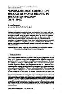
Figure 5: Permutation codewords based on Hadamard matrices.
As an example, consider n = 27 and k = 4. We have ⎛ ⎜ H =⎜ ⎜ ⎝
1 1 1 −1 1 1 1 −1
1 1 ⎞ 1 −1 ⎟ ⎟ −1 −1 ⎟ −1 1 ⎠
and s = 3. Four codewords of the code based on this Hadamard matrix are plotted in Figure 5.5. √ Another construction based on [2] holds for 3 ≤ k ≤ n, leading to k permutations with minimum 1/3 translocation distance at least n − 32 (kn) . The construction is described below.
Let s = (n/k 2 ) and s′ = (nk) and assume s and s′ are integers. Consider the integer lattice ′ ′ [s] × [s − 1] × [s − 1] denoted by X. Let φn,k ∶ [n] → X be such that (x, y, z) = φk,n (m) if and only if 1/3
1/3
(m − 1) = (x − 1) + s (y − 1) + ss′ (z − 1) .
Let the smallest prime larger than 4s′ be denoted by p. For i ∈ [3] and j ∈ [k] define gi,j ∶ X → Z as g3,j (x, y, z) = j 2 + 2jy + 2z g2,j (x, y, z) = jx + y,
(mod p) ,
g1,j (x, y, z) = x,
and let hj = (g1,j ○ φn,k , g2,j ○ φn,k , g3,j ○ φn,k ). Each hj defines a total ordering