Oct 27, 2016 - Index TermsâDense and Big Data, Large-Scale Distributed. Computing, Iterative Machine Learning, Subspace Factorization.
RankMap: A Platform-Aware Framework for Distributed Learning from Dense Datasets Azalia Mirhoseini1 , Eva. L. Dyer2 , Ebrahim. M. Songhori3 , Richard Baraniuk4 , and Farinaz Koushanfar1
arXiv:1503.08169v1 [cs.DC] 27 Mar 2015
Dept. of Electrical and Computer Engineering, Rice University, Houston, TX1,3,4,5 Dept. of Physical Medicine and Rehabilitation, Northwestern University; Rehabilitation Institute of Chicago2
azalia1 , ebrahim3 , richb4 , farinaz5 @rice.edu edyer2 @ric.org ABSTRACT
examples of such algorithms and their applications are linear or penalized regression, power iterations, belief propagation, and expectation maximization [1, 2]. In all of these settings, solving the underlying objective function requires iterative updates of parameters of interest until convergence is achieved. Such iterative updates often require matrix multiplications that involve the data dependency or Gram matrix. In scenarios where data is too large to fit on a single computing node and must be distributed, iterative dependencybased updates become highly challenging as they incur large computation and communication costs. A number of distributed abstractions that target iterative learning algorithms have been developed, e.g., Pregel [3], and GraphLab [4]. These abstractions adopt a graphparallel model which consists of a sparse graph and a kernel function that runs in parallel on each vertex [5]. Performance gains are achieved due to the communicationminimizing partitioning of the graph and effective control of data movement. While graph-parallelism has been shown to accelerate machine learning and signal processing tasks for sparse graphs, this approach cannot be readily applied when the data exhibit a non-sparse dependency matrix. The storage of such data in the graph format becomes very inefficient as it requires storing large number of edges (corresponding to dense dependencies) for each vertex. In addition, finding efficient graph cuts and partitions is infeasible when dense dependencies exist. Data with dense dependencies appear in a wide range of important fields such as computer vision, medical image processing, the boundary element methods and their applications, and N-body problems [6, 7]. Thus, finding efficient solutions for running iterative learning algorithms on densely dependent data is of paramount importance. In this paper, we introduce RankMap, a novel distributed framework for efficient execution of a broad class of iterative learning algorithms on datasets with dense dependencies. Our key observation is that, despite the apparent high dimensionality of data, in many settings dense datasets are low rank or lie on a union of much lower dimensional subspaces. We exploit this property to reduce the overhead of data dependencies, a factor which has rendered the currently available graph-parallel abstractions impractical for processing dense datasets. RankMap provides a set of interfaces and transformations that enable efficient data-aware content analysis, as well as coordinated mapping and optimization of the underlying hardware components. Our
This paper introduces RankMap, a platform-aware end-toend framework for efficient execution of a broad class of iterative learning algorithms for massive and dense datasets. In contrast to the existing dense (iterative) data analysis methods that are oblivious to the platform, for the first time, we introduce novel scalable data transformation and mapping algorithms that enable optimizing for the underlying computing platforms’ cost/constraints. The cost is defined by the number of arithmetic and (within-platform) message passing operations incurred by the variable updates in each iteration, while the constraints are set by the available memory resources. RankMap transformation scalably factorizes data into an ensemble of lower dimensional subspaces, while its mapping schedules the flow of iterative computation on the transformed data onto the pertinent computing machine. We show a trade-off between the desired level of accuracy for the learning algorithm and the RankMap’s achieved efficiency. RankMap provides two APIs, one matrix-based and one graph-based, which facilitate automated adoption of the framework for performing several contemporary iterative learning applications optimized to the platform. To demonstrate the utility of RankMap, we solve sparse recovery and power iteration problems on various real-world datasets with up to 1.8 billion non-zeros. Our evaluations are performed on Amazon EC2 and IBM iDataPlex platforms using up to 244 cores. The results demonstrate up to 2 orders of magnitude improvements in memory usage, execution speed, and bandwidth compared with the best reported prior work.
1.
INTRODUCTION
Many modern learning algorithms are based on exploring the underlying patterns, correlations, and dependencies present across the signals in the dataset. Some prominent
1
overarching goal is to reduce the following critical metrics in high performance distributed computing systems: execution runtime, memory usage, and communication overhead. To accelerate matrix vector multiplications required to compute an iterative update, we decompose dense but structured data and rewrite it as a product of two matrices with far fewer non-zeros than the original data. The shrunk decomposed data is then used in subsequent iterative learning algorithms. We introduce a host of automated methods for partitioning the decomposed factors and ordering the computation flow in a distributed setting. The partitioning algorithm is efficient (within a bound from the optimum) and has a constant runtime. We introduce two different representations and accompanying computational models (a matrix-based and a vertex-centric model) to compute an update. We show that depending on the data domain and the sparsity of the decomposed components, there are different regimes where each of these two models deliver highest efficiency. We provide APIs for both matrix-based and vertex-centric iterative update models on the transformed data. Our matrix-based API uses the general Message Passing Interface (MPI). Our vertex-centric API is written based on the GraphLab programming model. We develop an efficient mapping of the iterative computations on the sparsified decomposed data within the constraints of the GraphLab distributed framework. Both APIs are written in C++. We evaluate RankMap on the Amazon Elastic Cloud(EC2) computing service and the IBM iDataPlex computer cluster. Our experiments utilize up to 244 cores on 12 large computing nodes. The RankMap APIs are open source and shall be freely available to download (hidden to observe anonymity). Our explicit contributions are as follows:
Figure 1: Schematic depiction of decomposing dense data dependencies into a large sparse component and a small dense one.
computational models.
2.
RankMap FRAMEWORK
2.1
Overview and approach
In this paper, we introduce RankMap, a distributed dataaware framework that efficiently executes learning algorithms that rely on costly iterative updates on dense Gram matrices. The main idea underlying our approach is to leverage structure in large collections of data to decompose the Gram matrix such that the system costs (e.g, runtime, memory, and energy) associated with iterative learning algorithms are significantly reduced. Let the data matrix A ∈ Rm×n denote a collection of n signals of m-dimensions, and G = AT A denote the Gram matrix. Many learning algorithms iteratively update a solution vector, denoted by x, according to an update function of the following form: xiter+1 = f (Gxiter ),
(1)
where f (·) is a low-complexity function. When G is massive and dense, each distributed update becomes very expensive. Thus, RankMap creates an approxib to reduce the cost of an update. mation to G, denoted by G, To be more specific, our aim is to decompose the data mab = DV, where D ∈ Rm×l trix A into two components, i.e., A contains a subset of columns from A, V ∈ Rl×n is a sparse matrix, and rank(A) ≤ l � n (Figure 1). After decomposing A, we then efficiently partition the decomposed data b = (DV)T (DV). and perform distributed updates using G Mapping the original dense data to a decomposed model directly reduces the memory usage, and the costly computational operations and communication incurred by the iterative updates. When A is exactly low rank (single low-dimensional subspaces) or lies on a small number of low-dimensional subspaces, the aforementioned decomposition is exact. However, we demonstrate that for many real-world datasets, we can achieve significant performance improvements in exchange for a small decomposition error. We discuss the connection between the decomposition error and the accuracy of a target learning method as well as strategies for tuning the decomposition to achieve a desired level of accuracy in the iterative learning algorithms. Figure 2 shows an overview of the our framework. RankMap consists of three main components: (i) A scalable data decomposition that shrinks the size of the domain content by leveraging the data’s structured properties, (ii) A data partitioning scheme along with an execution flow for performing iterative updates on the decomposed data that significantly reduces the distributed computing costs, (iii) a
• We propose the RankMap framework, a suite of domain-specific transformations and distributed interfaces that enable executing a large set of popular knowledge extraction algorithms on big and dense data. Based upon learning the domain data, dependency structure, and the properties of the underlying hardware, RankMap provides an efficient resourceaware mapping of the computation onto the distributed setting. • (Section 4) We introduce a novel scalable transformation which maps a dense and structured data onto two matrices which contain fewer number of non-zeros. The resulting decomposition can be used for improving the performance of several important iterative learning algorithms that exploit data dependencies. We provide a systematic way to tune the decomposition error to achieve a desired level of accuracy in the learning applications. • (Section 5) We develop efficient distributed computational models to conduct iterative updates on the decomposed data. Highly effective partitioning methods for the decomposed data along with data-aware performance bounds are provided. • (Section 6) We perform proof-of-concept evaluation on applications including eigenvalue decomposition, denoising, and classification that demonstrate up to 2 orders of magnitude improvement in runtime and memory footprint. • (Section 7) We discuss the practicality of RankMap and domain-specific use-cases of each of the proposed 2
Figure 2: An overview of RankMap framework.
systematic method for tuning the decomposition error (denoted by δD ) to achieve the desired level of approximation error in the learning algorithms (denoted by δL ).
2.2
iterative update: xiter+1 =
Target applications
(i) Sparse approximation for image denoising and classification. Sparse representation is used in a wide range of signal processing and machine learning applications, including denoising [8] and more recently in classification [9]. For example, in an image denoising application, y is a noisy image and Ax is a denoised approximation of y. In a classification application, the sparse coefficient vector x is used to determine which class a test signal y belongs to. This is done by first measuring the sum of the coefficients in each class and then finding the class that has maximal coefficient energy. In the sequel, we evaluate the performance of RankMap for accelerating first-order methods for `1 -minimization. This objective can be written as follows:
Other applications. Our framework can be used for a broad class of optimization problems that are solved via iterative updates based upon the Gram matrix. For instance, projected gradient descent (PGD) methods which provide a generalization of standard gradient descent methods for certain classes of non-smooth objective functions, can also benefit from RankMap. A large number of machine learning objective functions and penalized regression methods such as the LASSO or BPDN [8], and Ridge regression [12] can be solved via a PGD approach. In all these settings, RankMap can efficiently handle the costly iterative computations based on the distributed Gram matrix.
(2)
x
where the solution x is a sparse representation of y with respect to A and λ is a regularization coefficient (increasing λ results in sparser solutions). This sparse approximation problem can be solved using the following iterative algorithm: iter+1
x
= f (x
iter
− γ(Gx
iter
T
− A y)),
(4)
Once the power method converges to an estimate of an eigenvector x, the contribution of this eigenvector is removed from A, and the power method is applied again to the residual to find the next eigenvector. In both applications described above, the main cost of each iteration is due to the computation of Gx, as G is dense, massive, and distributed onto multiple computing nodes. For example, as a case-study in our evaluations, we conduct image reconstruction on a dataset where A is a collection of light field image patches of size 18k × 100k. In this case, to reconstruct a single noisy image patch y, more than 3.6 billion floating point multiplications are required to perform Gx = AT Ax per iteration.
To ground RankMap in real-world problems, we now discuss two particular learning algorithms that are evaluated in this paper: (i) sparse approximation and (ii) the power method for eigenvalue decomposition.
arg min kAx − yk2 + λkxk1 ,
Gxiter . kGxiter k2
3.
BACKGROUND AND RELATED WORK
In this section, we provide background on methods for matrix factorization and describe related work.
(3)
where f (.) is a low-complexity thresholding operation (e.g., a soft-thresholding operator [10]) to account for the term λkxk1 at each iteration and γ is the step size. In our evaluations, we employ an accelerated variant of this algorithm called FISTA [11].
3.1
Methods for matrix factorization
High-dimensional data often can be well modeled by the low rank structures that are present in the data. Extracting low dimensional structures not only reduces dimensionality, but also mitigates the effect of high-dimensional noise and improves the performance of learning and inference tasks [13].
(ii) Power method for eigenvalue decomposition. The power method is a simple and iterative algorithm that can be used to sequentially find the eigenvectors and eigenvalues of a matrix in descending order. Recall that an eigenvector x of a matrix A satisfies the following relationship Ax = λx, where λ is the eigenvalue associated with the eigenvector x. To find an eigenvector of the symmetric matrix G = AT A, the power method utilized the following
3.1.1
Singular value decomposition (SVD)
In settings where the column span of A admits a low rank model, the SVD provides a powerful tool for forming low rank approximations. The best rank-k approximation of A is given by Ak = Uk Σk VkT , where Uk ∈ Rm×k and Vk ∈ 3
Rn×k are the truncated singular vectors (first k columns of U and V) and Σk ∈ Rk×k contains the first k singular values of A along its diagonal. The rank equals the number of non-zero singular values or rank(A). The truncated SVD also provides the solution to principal components analysis (PCA), which seeks to find a k-dimensional subspace that best approximates A in the least-squares sense. The complexity of computing the SVD directly is m2 n. Thus, for large datasets, the power method is used to find the eigenvectors of AT A and AAT , which correspond to the right and left singular vectors respectively.
3.1.2
densely connected, the resulting communication congestion makes the computation dramatically slow. Because of this, most of these tools are designed based on the assumption that the input data is sparse [5, 3, 21].
4.
In this section, we present a scalable method for matrix decomposition (the Decomposition phase in Figure 2) which we call Subsampled Sparse Matrix Decomposition (CSSD).
4.1
Sparse factorization
4.1.1
Step 1. Sequential column selection
In order to ensure that the total approximation error in our factorization is sufficiently small, we must ensure that the columns selected from A to form D well approximate the range of the original matrix. Thus, a number of column sampling approaches employ a sequential method to adaptively select columns that are not well approximated by the current set of columns [24]. Adaptive column selection methods consist of two main steps. First, we compute the projection error E = A − AS A+ S based upon the current set of selected columns given by AS 1 . Second, we select a new batch of columns according to the following probability distribution:
Column subset selection (CSS)-based matrix factorization
In contrast to methods such as PCA and its sparse variants, an alternative strategy for low rank matrix factorization is to form a decomposition based upon columns (or row) from the data. CSS-based solutions form an approximate matrix decomposition in which one factorized component is a subset of the columns of the data itself [17]. CSS-based approaches have been used to provide a scalable and efficient strategy for finding approximate solutions to least-squares regression [18], Gramian matrix decomposition [17], and also in spectral clustering [19]. In all of the aforementioned settings, CSS is employed to select a few columns from A and a low rank decomposition is obtained by projecting the data onto the subspace spanned by this set of columns. Our proposed data decomposition approach leverages a CSS-based to form the left factor matrix D.
p(i) ∝
kAS A+ S ai − ai k2 , kai k2
(5)
where p(i) equals the probability of selecting the ith column from A, given by ai . This subsampling approach can be used by either specifying the maximum number of columns to select and/or specifying the maximum amount of error in each column of A.
4.1.2
3.2
Overview of CSSD method
The main idea behind CSSD is to: (i) select a subset of columns from a matrix and (ii) use this subset of columns as a basis from which we form sparse representations of the remaining columns in the dataset. To be precise, if we consider a factorization of A = DV, the matrix D is formed by subsampling and normalizing columns of A and each column of V is computed by finding the sparse approximation of the corresponding column of A with respect to D. This sparse approximation problem can be solved by an efficient greedy routine called orthogonal matching pursuit (OMP) [23]. We provide pseudocode for CSSD in Alg. 1.
The SVD provides a closed-form solution for finding the best rank-k approximation to a matrix. However, in many settings, enforcing sparse structure, either in the left or right singular vectors can provide a more faithful and compact decomposition of the data. Two widely used sparse factorization methods include sparse PCA (SPCA) [14] and dictionary learning (DL) [15]. However, these approaches are often not applied to large datasets since computing an update of both the left and right factor matrices, at each iteration is costly. To solve SPCA on big datasets, a generalized power method can be employed [16]. The basic idea behind using the power method to find sparse principal components is to simply threshold the output of each power iteration to ensure the resulting eigenvectors are sparse. Unfortunately, the convergence of this method is much slower than standard power iterations.
3.1.3
COLUMN SELECTION-BASED SPARSE DECOMPOSITION (CSSD)
Generic distributed abstractions
Step 2. Sparse approximation
After selecting a subset of l columns AS ∈ Rm×l , we normalize each column to produce a matrix with unit norm columns D. Now, to form the sparse matrix V, we find a sparse representation of the remaining columns in A (i.e., A−S ) in terms of the normalized dictionary D. The problem is formally written as follows:
A number of successful distributed abstractions for processing large datasets on clusters have been proposed. Examples include MapReduce [20], Apache Spark [21], and SystemML [22]. However these models become less efficient for applications when direct data-parallelism does not exist. Several new distributed abstractions have been proposed that model data dependency in a graph format, most notably Pregel [3] and GraphLab [4]. They use a vertex-centric computation model, in which the user-defined programs are executed on each vertex in parallel. However, graph-based abstractions are suited for sparse datasets as efficient data partitioning is not possible when data is densely connected. Furthermore, such tools mostly rely on the communication between the vertices for computation. When the data is
ka − Dvk2 ≤ δD . kak2 (6) We employ a matching pursuit-based solver called Batch OMP [25] to solve Equation 6. The solver allows us to enforce sparsity either by fixing the number of non-zeros in ∀ a ∈ A−S solve:
1
4
min v
kvk0
s.t.
The pseudo-inverse is calculated as: A+ = (AT A)−1 AT .
Algorithm 1 : CSSD
is approximately low rank, there exists a large body of work that characterizes the performance of the sequential column selection method (Step 1) used to form D. In particular, the selection strategy in Step 2 of Algorithm 1 provides exponential decrease in the factorization error with each batch of columns that we select from A [24]. More specifically, assume that at each iteration, we select ls > r� samples from the columns of A and let l = tls denote the set of columns selected after t iterations. Let Ar denote the best rank r e = AS A+ A denote the apapproximation to A and let A S proximation of A based upon the l selected columns. Then according to [24], the difference between the expected value e 2F and that of the of the approximation error, i.e., kA − Ak 2 best rank r approximation kA − Ar kF decreases exponentially with rate �t . Another low-dimensional signal model that has recently gained traction captures a collection of data with multiple low-dimensional subspaces (union of low-dimensional subspaces). For example, images of objects under different illumination conditions [26], motion trajectories of point-correspondences [27], to structured sparse and block-sparse signals [28] are all well-approximated by a union of low-dimensional subspaces. When A lies on a union of subspaces, this effectively bounds the sparsity level of each column of V [29]. This insight is based upon the fact that when we form a representation of a column of A with respect to other columns in the same dataset (as in CSSD), the sparsity level of each column is bounded by the dimension of the subspace the signal lies on. For instance, if A lives on a union of multiple r-dimensional subspaces of Rn and we select at least r linearly independent columns from each subspace, then no more than r non-zeros must be used to represent a signal. In other words the number of non-zeros per column of V is no more than r.
m×n
Input: Matrix A ∈ R , error tolerance δD , number of columns to select at each iteration ls , and the maximum number of columns to select l. Output: A sparse matrix V ∈ Rl×n and a dense matrix D ∈ Rm×l such that for each column of a of A, ka − Dvk2 ≤ δD . Initialize: Initialize D by adding and normalizing ls columns from A with uniform random sampling. Step 1: Sequential column selection while ncols(D) < L do I. Update D by selecting and normalizing ls columns from A according to the distribution in Equation 5. II. If the `2 -norm of each column of E = A − DD+ A is less than δD , return D and proceed to Step 2 to compute V. end while Step 2. Sparse approximation I. Compute V by applying Batch OMP to solve Equation 6 with error tolerance δD .
each column of V (i.e., kvk0 ) or by fixing the total amount of approximation error for each column (i.e., δD ).
4.2
Complexity analysis
The complexity of sequential column selection (Step 1) is O(l2 m + lmn). The complexity terms in turn correspond to computing D+ and DD+ A. For each column a of A, DD+ a can be computed independently. The complexity of sparse approximation (Step 2), using the Batch OMP method [25], is O(lmn + k2 ln), where k < l is the average number of non-zeros per column of V. Similarly, for each column a of A, Batch OMP is applied independently. Let nc be the number of parallel processing nodes. By storing D (which is a small m × l matrix) and a uniform fraction of columns of A in each node (i.e., nnc columns), the overall complexity of Algorithm 1 in a distributed setting can be written as O( nnc (lm + k2 l) + l2 m). Note that the scalability of CSSD is a crucial property which makes our framework applicable to very large datasets (large n) in distributed settings.
4.3
Impact of increasing the decomposition error δD . The decomposition error of CSSD is controlled by the parameter δD in Algorithm1. In the case where we set δD = 0, then we are guaranteed an exact decomposition of the data. Exact decomposition occurs when m linearly independent columns are selected from A; in this case, the selected columns in AS will span the ambient dimension of the data Rm and thus kA − AS A+ S Ak = 0, i.e., exact decomposition occurs. While CSSD can produce an exact and compact decomposition when the data is exactly low rank (or lies on a union of subspaces), in practice, datasets are approximately low rank. In this case, we can introduce a small amount of error into the decomposition by setting δD > 0. By introducing some error into the decomposition, we observe that both the number of selected columns in Step 1 of Algorithm 1 and the sparsity level of V can be reduced further. In Figure 7 we show how increasing the decomposition error produces a more compact result.
Computational benefits of CSSD
CSSD provides computational benefits when the size of the decomposition is small (i.e., l is small relative to m) and/or when matrix V is sparse. In general, predicting the amount of savings in computation is a function of (i) the structure of the data and (ii) the amount of accuracy required from the learning algorithm. We now discuss some key factors that impact the decomposition results. Impact of data structure. Predicting the size and sparsity of the decomposition provided by CSSD for an arbitrary dataset is challenging; however, when the data lies on a single subspace (i.e., exhibits low rank structure) or lies on multiple low-dimensional subspaces, CSSD provides a more compact representation of the data. For example, for when data is exactly low rank and its rank is r < m, we must select r linearly independent columns from A to form an exact decomposition (zero error), i.e., l = r. When the data
4.4
Impact of decomposition error on learning accuracy
In the previous section, we discussed the computational benefits associated with introducing some approximation error into a CSSD decomposition. Naturally, as we increase the decomposition error (controlled by δD ) the accuracy of our learning algorithm (learning error) also increases. Thus, the key question is how much decomposition error we can 5
afford to achieve a certain degree of accuracy in learning. The answer to this question heavily depends on the specific learning algorithm and the application of interest. Previous theoretical work have established a connection between the total error in a factorization of a kernel (or Gram) matrix (δD ) and the accuracy of certain popular learning algorithms, including: kernel ridge regression and kernel SVM [30]. While for some learning algorithms, our framework can exploit the existing work in the literature to relate δD and the learning error which we denote by δL , the aim of this section is to propose a generic approach for tuning the factorization error to achieve a specified learning accuracy. In the following we introduce an approach for iteratively remapping of the data to find a compact decomposition that satisfies a pre-specified amount of learning error.
4.5
Figure 3: Distributed design of matrix-based model.
We propose two computational models for the distributed implementation of an update in Equation 1. Recall that at each iteration, we must compute z = Gx = VT (DT D)Vx. We break this computation into four steps: (i) p = Vx (ii) r = Dp, (iii) p = DT r, and (iv) z = VT p. The output vector z is used to produce an update of xiter+1 = f (z + b), where b is a constant and f (·) is a low-complexity function such as a soft-thresholding operator (sparse approximation) or normalization (power method). To carry out the computation described above, we propose and implement a matrix-based and vertex-based model to apply the iterative updates on the decomposed factors. We now describe our implementation of both models.
Error tuning
Given an already established relationship between the decomposition error and a specific algorithm, a practitioner who uses our framework can easily specify the error parameter δD for CSSD to achieve a particular learning accuracy. Alternatively, if a practitioner specifies a target accuracy for a learning algorithm, the decomposition error δD can be tuned in order to achieve a particular learning error δL . Our strategy for guaranteeing that we have small δL , is to solve CSSD for a particular δD , map the resulting decomposition via the methods described in Section 5, and then approximate the accuracy of a learning algorithm δL . Once the decomposition error δD is small enough then we can ensure that δL is small as well. Depending on the underlying computing resources available, RankMap can be applied for multiple values of δD in parallel and the largest value of δD (most compact representation) that achieves a particular value of δL is selected. When computing resources are constrained and thus running the algorithm for multiple values of δD in parallel is not possible, we use the bisection method. In essence, the idea is to: (i) set the factorization error to predefined maxmax (0.4 in our experiments) and evaluate δL , imum value δD (ii) if δL is below a target value then we stop, otherwise we decrease δD by half. By exponentially decreasing δD , we are also guaranteed to decrease δL exponentially, provided that there is a polynomial relationship between the two variables. We observe a polynomial relationship holds both in theory [30] and in practice. In Section 6, we supply empirical results which demonstrate the connection between the decomposition error and learning accuracy for numerous datasets and algorithms of interest (see Figures 6b and 7b).
5.
5.2
5.2.1
Distributed partitioning
We partition columns of V uniformly across the computing nodes to achieve a balanced partitioning. Let us assume that there are nc computing nodes. Thus, nnc number of columns are assigned to each node. Vector x is also divided into chunks of size nnc × 1. Each chunk is then allocated to the node that hosts the corresponding columns of V. Matrix-vector multiplications Vx are performed locally on the columns of V and portion of x that reside on the same computing node. The resulting l × 1 vectors are then sent to a central node to create p = Vx. Next, DT (Dp) is computed locally in the central node. The resulting l × 1 vector is then broadcasted back to all the computing nodes where it is multiplied by the local VT to update the vector x.
DISTRIBUTED EXECUTION AND DATA PARTITIONING
5.2.2
In this section, we introduce our approach for applying iterative updates on the decomposed data (the execution phase in Figure 2). We describe an execution flow for dependency-matrix based updates, i.e., Gx = VT (DT D)Vx, and introduce an efficient method for partitioning the decomposed data in a distributed setting. We also provide performance bounds on memory usage, number of flop operations, and number of communicated bytes across the computing nodes.
5.1
Matrix-based model
Figure 3 shows the schematic of our proposed matrixbased model. In this model, data is stored as arrays. Sparse matrix V is stored and operated upon using the Compressed Sparse Column (CSC) format. Matrice D and vector x are storred using regular dense arrays. By doing so, we exploit sparsity in V. We use C++ Eigen Library for array manipulation and MPI for distributed computing.
Performance bounds
We now provide bounds on the memory usage, computation, and communication required by our proposed matrixbased model. Let nnz(.) denote the number of non-zeros of its input and nc denote the number of computing nodes. Recall that D is a m × l matrix and V is a l × n matrix. • Memory usage # non-zeros ∝ (nnz(V) + lm) + n + m. • Computation (per iteration) # additions ∝ 2(nnz(V) + lm + lnc ) # multiplications ∝ 2(nnz(V) + lm)
Computation flow 6
tribute master of vertices Xi ∈ SX uniformly onto the available computing nodes such that vertex chunks of size nnc are assigned to each node. (ii) Add the edges between vertices Xi ∈ SX and Pj ∈ SP to the node in which the corresponding master of Xi resides. (iii) Add master of vertices Pi ∈ SP and R1 ∈ SR to a central node. and (iv) Add the edges between the vertices Pi ∈ SP and R1 ∈ SR to the central node. The proposed edge partitioning algorithm is highly efficient in that it does not induce any replicas for vertices in SX and SR . However from Step (ii) of the algorithm, replicas of vertices in SP may exist in computing nodes other than the central node. At the beginning of an iteration, master vertices in SP and their replicas perform vertex updates with respect to SX . The replicas send the updated values to their own master vertices in the central node. The master vertices in SP reduce the received values (p = Vx). Then master vertex R1 performs a vertex update (r = Dp − y). Next master vertices in SP complete vertex updates with respect to SR and broadcast the results to their own replicas (p = DT r). Finally master vertices in SX update themselves (x = VT p). We integrate and implement the proposed customized partitioning and distributed computation flow with the distributed GraphLab API [5].
Figure 4: Distributed design of graph-based model.
• Communication #edges ∝ 2lnc . Since matrix V is stored in a CSC format, only the nonzero values are stored and operated on. Matrix D is stored in a regular dense matrix format. The communication corresponds to sending and receiving the l × 1 vectors from each computing node to the central node. As can be seen, for smaller l and sparser V, both memory footprint and the numer of arithmetics is reduced. The number of edges, which correspond to the number of broadcasted and reduced values, directly corresponds to l and the number of computing nodes nc .
5.3
Graph-based model
5.3.2
Figure 4 shows an schematic of the graph model. The decomposed data graph denoted by GA (SX , SP , SR ) is a 3layer graph with vertex sets SX = {Xi }n i=1 in the bottom layer, SP = {Pi }li=1 in the middle layer, and SR = {R1 } in the top layer. Each non-zero element in V, e.g., Vij , is represented by an edge which connects Xi to Pj . Each column of D, e.g., Di , is represented by an edge which connects Pi to R1 . Value of vertices in SX correspond to the elements of x. We use GraphLab Distributed API [4] to implement this model. While GraphLab is a highly optimized distributed engine for Graph-based computation on iterative data, we perform extensive customizations in order to adapt GraphLab to our factorized setting. We also force GraphLab to use our developed graph partitioning method as opposed to its automated partitioning schemes. Our proposed partitioning is customized to the factorized data and significantly improves the performance.
5.3.1
Performance bounds
We now provide bounds on the memory usage, computation, and communication required by our proposed graphbased model. • Memory usage # edges ∝ nnz(V)P+ l. # vertices ∝ n + 1≤i≤l rep(Pi ). • Computation (per iteration) P # additions ∝ 2(nnz(V) + ml) + 1≤i≤l rep(Pi ). # multiplications ∝ 2(nnz(V) + ml). • Communication P # edge-cuts ∝ 2 1≤i≤l rep(Pi ). Each Pof the computing nodes receive approximately 1 1≤i≤l rep(Pi )) vertices and nc nnz(V) edges. The central node has l additional edges between the master vertices in SP and R1 . The computation cost is induced by vertex update operations. The communication overhead is incurred by the message passing across master and replica vertices in SP . Bound on total replicas. From above discussions, it is clear that reducing number of replicas of SP reduces the communication overhead. The following P are the bounds on the total number of replicas: l ≤ 1≤i≤l rep(Pi ) ≤ lnc . The inequalities hold since each Pi is replicated at least once and at most nc times (one replica per computing node). Both l and nc are much smaller than the size of the graph. Thus, RankMap’s graph-based model readily provides efficient/balanced computation and reduced communication without using complicated and costly graph partitioning algorithms. The minimum communication is achieved when V is block-diagonal. 1 (n + nc
Distributed partitioning
In the graph-based model, we partition GA (SX , SP , SR ) with the aim of balancing the number of components assigned to each node and also minimizing the inter-node communications characterized by the edges. Since the edge distribution of GA is highly non-uniform (l � n), a vertex partitioning inevitably results in many undesirable edge-cuts across the computing nodes. Instead, we apply a vertex-cut method in which the goal is to partition graph edges evenly such that the number of vertices that are spanned across multiple partitions is minimized. As a results of edge partitioning, in our implementation, vertices may reside onto two or more computing nodes. In this case we assign one of the copies to be the master vertex and the others to be the replica vertices (these definitions are borrowed from GraphLab [5]). The replicas directly cause (expensive) internode communication costs. Figure 4 shows the graph-based distributed design. Our detailed edge partitioning method is as follows. (i) Dis-
6.
EVALUATIONS
In this Section, we evaluate the performance of RankMap on a diverse set of real-world and synthetic datasets. The real datasets include Light Field data from [31], hyper spectral images from [32], a dictionary of video frames from [33], 7
and a collection of images of different faces under varying illumination conditions [34]. We study the the scaling behavior of CSSD, the connection between decomposition error and learning accuracy, and timing and performance of our distributed matrix and graph-based models.
6.1 6.1.1
Figure 5 shows how the runtime of CSSD scales as the number of processors increases for the VideoDict dataset. We increase the number of cores from 4 to 256 (on IBM iDataPlex cluster). The dotted line shows the ideal scaleout behavior. As can be seen, CSSD is highly parallel as it almost linearly scales with the number of processors. Thus, it can be applied to very large datasets.
Evaluation setup Datasets
We apply RankMap to two different light field datasets. The first dataset, which we refer to as Light Field (i), consists of 10k randomly selected atoms from a 5 × 5 light field array (collected from Chess Images). Each light field patch consists of 25 8 × 8-patches which produces a dataset of size 1.6k × 10k (128M B). The second dataset, which we refer to as Light Field (ii), consists of 100k randomly selected atoms from a 17 × 17 light field arrays (collected from all available light fields in the archive). Each light field patch consists of 289 8 × 8-patches which produces a dataset of size 18496 × 100k (14.7GB). The hyper spectral dataset (Salinas) is taken from a region of a remote sensing scene in Salinas, CA; each pixel in the scene contains information from 203 spectral bands and produces a dataset of size 203×54129(87.9M B). The video dictionary dataset (VideoDict) contains patches of an image over multiple frames and produces a dataset of size 1764×100000 (168M B). The face image dataset (Faces) consists of 631 images of 10 different peoples faces under varying illumination conditions. Each image is 48 × 84 pixels, which produces a dataset of size 4032 × 631. In addition to real-world datasets, we generate synthetic decomposed data for n = 10M , m = 1k with varying l and sparsity levels in V.
6.1.2
Relative Speedup
102
4
8
16 32 64 # of Processors
128
256
Figure 5: CSSD’s runtime scaling behavior as the number of processors increases.
6.3
Sparse approximation
To evaluate the performance of RankMap for sparse approximation, we use the fast iterative shrinkage-thresholding algorithm (FISTA) [11] to solve the `1 -minimization problem in Equation 2. We study the utility of RankMap for two applications of the sparse representation problem discussed in Section 2.2. The applications include, sparse representation-based classification for face recognition and image denoising.
Computing platform
6.3.1
Sparse representation-based classification for face recognition
To employ sparse approximation for classification, our aim is to use a collection of labeled images (training set) as our dictionary A and then form a sparse representation of a test image y in terms of A. Upon finding a sparse coefficient vector x which provides a sparse approximation of y ≈ Ax, we can then determine which test signals (columns of A or non zeros in x) are selected to represent the test signal y. Based upon the class of the selected columns, we then make a decision about which class the test signal lies in. One easy way to do this is to simply sum the absolute value of the coefficients in x in a certain class and then find the class that has the maximum sum. In Figure 6a, we provide a demonstration of sparse representation-based classification for face recognition. We show the test image of interest on top and the corresponding sparse coefficient vector obtained by solving Equation 2 with FISTA for λ = 1. We solve FISTA with the full Gram matrix AT A and approximate Gram provided by CSSD, where the decomposition error δD = 0.05 (l = 62). To understand the connection between the decomposition error and learning accuracy for face recognition, we solve Equation 2 using FISTA for two different regularization parameters λ = {0, 1}, where λ = 0 corresponds to the leastsquares solution and λ = 1 produces sparse solutions. We vary the decomposition error δD = {0.4, 0.2, 0.1, 0.05} and solve FISTA for 30 different test images (after removing them from training) for each of these decompositions. For
Distributed tools
The RankMap framework’s sparse graph-based design is implemented using GraphLab, a high-level graph-parallel abstraction [5]. GraphLab enables vertex-update-based computations. We implemented RankMap’s customized partitioning using Graphlab’s ingress class. The proposed architectures are mapped efficiently into GraphLab API (Section 5.3). Note that the GraphLab framework is designed to accelerate distributed learning for sparse graphs and thus it is not suited to process dense data until we sparsify the data using CSSD. The RankMap framework’s sparse matrix-based computations is implemented using Eigen library to represent data in a compressed column storage (CCS) format [35]. It uses MPI standard system to distribute the data and computation and is written in C++. We have also implemented the distributed update on the factorized data on Apache Spark [21].
6.2
101
100
To evaluate the decomposition methods on light field (i) an 8-core CPU (Intel CoreTM i7 processor) with 12GB of RAM is used. For computations on light field dataset (ii), a cluster of 16 m3.large nodes (machines) on Amazon EC2 is instanciated. Each node has 16 cores (two Intel Xeon processors) at 7.5GB of RAM per node. The synthetic datasets are evaluated on IBM iDataPlex computing cluster which has 2304 cores in 192 Westmere nodes (12 processor cores per node) at 48GB of RAM per node.
6.1.3
Ideal CSSD with l=1000
Scaling of CSSD 8
each decomposition, we calculate the: learning accuracy by measuring the `2 -norm between the solution obtained with the full and approximate Gram (Figure 6b), the sum of coefficients in the correct class (Figure 6c), and the relative density of V or the number of non-zeros in V versus the number of non-zeros in A (Figure 6d). In Figure 6c, we also display the minimum sum of coefficients required to correctly classify the test image. These results suggest that while learning accuracy might be relatively large for high amounts of decomposition error, correct classification is possible even for large amounts of decomposition error (i.e., correct classification occurs for all test images when δD < 0.2).
6.3.2
decomposed data. For example, while the baseline’s highest achieved PSNR at convergence is 48.5 dB, it is 31.3 dB and 38.5 dB for l = 240 and l = 1000 respectively. Table 1: FISTA runtime (s) to reach to a specific PSNR. PSNR (db) 25 30 35 40
Light field image denoising
6.4
We evaluate RankMap’s performance in solving the Light Field data reconstruction problem. In all the following experiments dataset Light Field (ii) is used. A light field is a multi-dimensional array of images. Each image is captured from a slightly different viewpoint. Combining the images enables creating new views and representing observer positions not present in the original array. Most currently available devices trade image resolution for the ability to capture different views of a light field. As a result, the final image resolution is reduced by orders of magnitude compared to the sensor resolution. To address this challenge, `1 -minimization (Equation 2) is employed to find a sparse representation of a light field image patch with respect to an over-complete light field dictionary consisting of a large number of light field image patches collected from many scenes [36]. We first apply CSSD for decomposing the dictionary corresponding to the Light Field (ii) dataset. Two different l values (240 and 1000) are used in Algorithm 1. The decomposition error δD is set to 0.1. We then evaluate FISTA on the decomposed data for matrix-based models. We also implement a tailored distributed MPI-based model to evaluate FISTA on the original datasets (A) using regular dense matrix representations. In the following, we refer to this model as baseline. Peak Signal to Noise Ratio (PSNR) is the ratio between the maximum possible power of a signal and the power of the corrupting noise. PSNR is most commonly used to measure the quality of reconstruction of noisy images and is defined M AX ) (dB). M AX is the maximum pixel value as 10 log10 ( √ 2 M SE of the original image patch and M SE is the mean square y |2 2 reconstruction error defined as |y−b . In our experiments m M AX = 0.0255. Generally, higher PSNRs indicate the better quality of reconstruction. Typical recommended PSNR values in image noise reduction application are 30 dB and higher [37, 38, 15]. Table 1 shows the total runtime of FISTA to achieve different PSNRs. In all the experiments, a batch of 10 noisy input patches is used as the input. The norm of the noise is 0.3 of the norm of the input vector (PSNR=21.14). It can be observed that by running FISTA on the decomposed data, the same PSNR is reached much faster in comparison with running FISTA on A. We observe that the runtime to achieve the same PSNR is orders of magnitude faster compared to the baseline. For instance, if our desired PSNR is 30.0 dB, running FISTA on the decomposed takes 13.9s (l=240) and 162s (l=1000) while it takes 1050s for the baseline. However, as expected, the baseline (A) reaches higher PSNRs in comparison with those achieved from running FISTA on the
l = 240 4.2 13.9 -
l = 1000 72 162 356 -
baseline (A) 487 1050 2051 3171
Power method
We also evaluate our framework on power method discussed in Section 2.2. Three datasets, namely Salinas, VideoDict, and Light Field (i) have been evaluated. The matrix-based mode is used and the experiments are run on 64 cores on IBMiDataplex server. We run CSSD with various decomposition errors (δD ) that belong to the following set: {0.4, 0.2, 0.1, 0.05, 0.001} and run power method on each of the decomposition results. Figure 7a shows the sparsity results as we vary the error. As expected, for larger error tolerances, a higher sparsity is achieved. Figure 7b shows the impact of the decomposition error on the accuracy of the results of the power method. Here the learning error (δL ) is defined to be the normalized accumulated error of the first 100 eigenvalues are achieved from running power method on the decomposed data versus those achieved by A (baseline). By lowering the decomposition error, we can observe significant improvements in the accuracy of the power method results. Finally, Figure 7c shows the corresponding normalized runtimes to find the first 100 eigenvalues. It can be observed that significant speedups in comparison with the baseline is achieved.
6.5
Graph- vs. matrix-based models
We compare the performance of RankMap’s proposed vertex and matrix-based models for various synthetic decomposed data. The purpose of these evaluations is to determine the advantage of each of the models with respect to the structure of the data. In all the experiments, the iterative update in Equation 3 is applied on a random input vector y. The experiments are done on an IBM iDataPlex computing cluster. In all the figures, the runtime results for the dense matrix-based implementation (i.e., regular deployment of the decomposed matrices without using CCS format) are also provided to demonstrate the efficiency achieved by exploiting sparsity in V through graph-based and sparse matrix-based models. Figure 8a shows the performance for different (blockdiagonal) V’s with fixed number of non-zeros (set to 100M ). Thus as l increases, the density-level of V would decrease. Graph-based model’s performance is more consistent as l increases. However, the matrix-based model’s performance degrades for larger l’s. This observation can also be explained due to the fact that the communication overhead of the matrix-based model is more affected by larger l’s. Figure 8b shows the performance for a fixed l = 500 on block-diagonal matrices V for varying densities of V. As density increases, the performance decreases in both models. However, the performance degradation in graph-based model is worse due to the overhead of representing a large 9
Test Image
0.4 Coefficients in Correct Class
0.025
Baseline (A) CSSD
0.02
Learning Error
Sparse Coefficients
0.8
0.015
0.6 0.4
0.005 0
100
200
300
400
Image Number
500
0.1
0.2
Decomposition Error
(a)
0.3
0.2
0.15
Least−squares L1−min
0 0
600
0.3
0.25
0.2
0.01
0.7
Least−squares L1−min Correct Class
0.35
Relative Density of V (%)
1
0.1
0.05 0
0.4
(b)
0.1
0.2
Decomposition Error
0.3
0.6 0.5 0.4 0.3 0.2 0.1 0 0
0.4
(c)
0.1
0.2
0.3
0.4
Decomposition Error
(d)
Figure 6: Sparse representation-based face recognition. (a) On top, we display a test image; on the bottom, we display the sparse solution obtained with the original Gram (blue, solid) and approximate Gram with CSSD for δD = 0.05 (red, dash). We display four training images corresponding to non zero coefficients: large amplitude coefficients correspond to images in the correct class and smaller amplitude coefficients correspond to images in incorrect classes. The block of coefficients corresponding to images in the correct class are highlighted. For a range of decompositions (varying δD ) we show (b) learning accuracy which measures the 2-norm between the solution obtained with the full and approximate Gram, (c) sum of coefficients in the correct class, the minimum sum of coefficients required to correctly classify the test image is also shown. and (d) relative number of non-zeros in V versus the number of non-zeros in A. 50
0.15 Salinas Light Field(i) VideoDict
60 40
Relative Speedup
80
Salinas Light Field(i) VideoDict
Learning Error
Relative Density of V (%)
100
0.1
0.05
30 20 10
20 0
Salinas Light Field(i) VideoDict
40
0
0.1
0.2 0.3 Decomposition Error
0.4
0
0 0
0.1
0.2 0.3 Decomposition Error
(a)
(b)
0.4
0
0.1
0.2 0.3 Decomposition Error
0.4
(c)
Figure 7: Power method results for three datasets: Salinas, VideoDict, and Light Field (i). Effect of varying the decomposition error (δD ) on (a) sparsity. Reported values are the number of non-zeros in decomposition factor V normalized to the number of non-zeros in A, (b) the learning error (δL ), and (c) the relative speedup of power method to find the first 100 eigenvalues. Relative values are runtime of power method using the decomposed factors derived from CSSD normalized to the corresponding runtime using A.
number of edges. Lastly, Figure 8c shows the scaling performance of the models for various number of processors. When the number of processors are less than 12, the computations are done on a single node. Thus the reverse scaling behavior while increasing the number of processors from 8 to 16 is due to the high overhead of the inter-node communication cost. For comparison purposes, the scaling performance of the baseline dense m = 1k by n = 10M dataset (before decomposition) is provided. It can be seen that as the number of processors increases, the performance gap between different methods shrink. However, even with a large number of processors (≥ 100), the decomposed models perform up to 2 orders of magnitude better than the baseline. These experiments provide insights on the use-case of each model. Depending on the structure of the decomposed data and the specifications of the platforms an appropriate model should be selected. A more systematic domain-specific approach for model selection is the subject of future work.
7.
This paper introduces RankMap, a novel distributed framework for applying a host of iterative learning algorithms on large-scale dense and structured datasets. Our framework leverages low-dimensional structure in datasets in order to map a large dataset with dense dependencies into lower dimensional components with sparse representations. Both matrix-based and graph-based distributed computational models were designed to efficiently carry out iterative update algorithms on the decomposed components. We provide guidelines on the use cases of each model based upon the decomposed data structures and the underlying computing platform. An efficient partitioning of the computational flow is developed that guarantees load balancing and significantly lowers communication overhead. We evaluate the performance of RankMap on sparse recovery and power method algorithms on various datasets and demonstrate significant improvements in runtime and memory footprint.
7.1
Decomposition overhead
RankMap applies the CSSD method offline and then uses the decomposed components for efficient execution of var-
CONCLUSION 10
10
0
102
103 104 Size of decomposition (l)
10
1
10
0
10
Runtime per iterations (s/iter)
10
Sparse matrix-based Dense matrix-based Graph-based
Runtime per iterations (s/iter)
Runtime per iterations (s/iter)
102 2
Sparse matrix-based Dense matrix-based Graph-based
-1
10-2 0.1
1 10 Relative density of V (%)
(a)
100
101 100 10 -1 10 -2 10 -3 10 0
(b)
Sparse matrix-based Dense matrix-based Graph-based Baseline 2
4
8
16
32
64
# of processors
(c)
Figure 8: Results on synthetic block diagonal data: (a) runtime vs. l, (b) relative density of V, and (c) number of processors.
ious iterative update algorithms. The performance gain achieved on the subsequent computations justifies the onetime decomposition overhead. For example, we decompose Light Field dataset (ii) (Section 6) on a cluster of 4 nodes (each with 12 cores) on IBM iDataPlex. For l = 240, the decomposition is completed in less than 15 minutes. For 10 sample patches (each of length 18k) the overall reconstruction time is reduced from more than 1000s to below 20s. Thus, the offline decomposition overhead can be justified once considering that there are thousands of patches in a single light field. Moreover, the same dictionary can be used to reconstruct other light field datasets.
7.2
ecution of iterative learning algorithms on big and densely dependent datasets. Whilst our decomposition method is very effective, the decomposition phase in RankMap (Figure 2) can be readily replaced by other sparse decomposition approaches.
8.
Model selection
In Section 5, we introduced a graph-based and matrixbased computational model; thus, it is natural to ask which model to select for data processing. Both models follow the same computational flow and operate only on the non-zeros. However, due to the higher overhead of the graph-based model for storing vertices and edges, it may consume more memory. The main advantage of the graph-based model instead is in its reduced communication cost. As discussed in Section 5.3.2, when V is approximately block diagonal, the communication cost in the graph-based model is reduced. In particular, when V is completely block diagonal the communication becomes almost independent of the number of computing nodes nc and is only proportional to 2l. In contrast, the communication cost in the matrix-based model is always proportional to 2lnc . This difference may result in a better overall performance of the graph-based approach, especially for larger l and nc values. In general, the performance of each model is highly dependent on the specifications of the available computing nodes. Our evaluations in Section 6.5 also provide insightful guidelines on the differences of the two models.
7.3
REFERENCES
[1] D. C. Montgomery et al., Introduction to linear regression analysis, 2012. [2] U. Nodelman et al., “Expectation maximization and complex duration distributions for continuous time bayesian networks,” 2012. [3] G. Malewicz et al., “Pregel: a system for large-scale graph processing,” SIGMOD, pp. 135–146, 2010. [4] Y. Low et al., “GraphLab: A new parallel framework for machine learning,” UAI, pp. 340–349, 2010. [5] J. Gonzalez et al., “Powergraph: Distributed graph-parallel computation on natural graphs,” OSDI, pp. 17–30, 2012. [6] K. Chen, “On a class of preconditioning methods for dense linear systems from boundary elements,” SIAM, pp. 684–698, 1998. [7] A. G. Gray and A. W. Moore, “N-Body’problems in statistical learning,” NIPS, pp. 521–527, 2000. [8] S. S. Chen et al., “Atomic decomposition by basis pursuit,” SIAM, pp. 33–61, 1998. [9] J. Wright et al., “Sparse representation for computer vision and pattern recognition,” IEEE, pp. 1031–1044, 2010. [10] I. Daubechies et al., “An iterative thresholding algorithm for linear inverse problems with a sparsity constraint,” CPAA, pp. 1413–1457, 2004. [11] A. Beck and M. Teboulle, “A fast iterative shrinkage-thresholding algorithm for linear inverse problems,” SIAM JIS, pp. 183–202, 2009. [12] A. E. Hoerl and R. W. Kennard, “Ridge regression: Biased estimation for nonorthogonal problems,” Technometrics, vol. 12, no. 1, pp. 55–67, 1970. [13] E. Elhamifar and R. Vidal, “Sparse subspace clustering: algorithm, theory, and applications,” TPAMI, pp. 2765–2781, 2013. [14] H. Zou, T. Hastie, and R. Tibshirani, “Sparse principal component analysis,” JCGS, pp. 265–286, 2006. [15] M. Aharon, M. Elad, and A. Bruckstein, “K-SVD: An algorithm for designing overcomplete dictionaries for sparse representation,” TSP, pp. 4311–4322, 2006.
Alternative decomposition strategies
While sparse matrix factorization approaches such as SPCA and KSVD have objectives similar to CSSD, their complexity make them inapplicable to massive datasets. Our proposed decomposition instead is fast and scalable. Our CSS-based approach creates the decomposition factor D from a subset of columns of A. However, both SPCA and KSVD require costly computations to create D which requires computing the SVD of the data. Note that in addition to proposing an scalable decomposition, our framework for the first time introduces and successfully implements the idea of creating error-tunable sparse decompositions for efficient ex11
[16] M. Journ´ee et al., “Generalized power method for sparse PCA,” JMLR, pp. 517–553, 2010. [17] P. Drineas and M. Mahoney, “On the nystr¨ om method for approximating a gram matrix for improved kernel-based learning,” JMLR, pp. 2153–2175, 2005. [18] P. Drineas, A. Frieze, R. Kannan, S. Vempala, and V. Vinay, “Clustering large graphs via the singular value decomposition,” JML, pp. 9–33, 2004. [19] C. Fowlkes et al., “Spectral grouping using the nystrom method,” TPAMI, pp. 214–225, 2004. [20] J. Dean and S. Ghemawat, “MapReduce: simplified data processing on large clusters,” CACM, pp. 107–113, 2008. [21] M. Zaharia et al., “Resilient distributed datasets: A fault-tolerant abstraction for in-memory cluster computing,” in USENIX NSDI, 2012, pp. 2–2. [22] A. Ghoting et al., “Systemml: Declarative machine learning on mapreduce,” in ICDE, 2011, pp. 231–242. [Online]. Available: http://dx.doi.org/10.1109/ICDE.2011.5767930 [23] G. Davis, S. Mallat, and Z. Zhang, “Adaptive time-frequency decompositions,” Opt. Engin SPIE, pp. 2183–2191, 1994. [24] A. Deshpande et al., “Matrix approximation and projective clustering via volume sampling,” in SIAM. ACM, 2006, pp. 1117–1126. [25] R. Rubinstein, M. Zibulevsky, and M. Elad, “Efficient implementation of the k-svd algorithm using batch orthogonal matching pursuit,” CS Technion, 2008. [26] R. Ramamoorthi, “Analytic PCA construction for theoretical analysis of lighting variability in images of a lambertian object,” TPAMI, pp. 1322–1333, 2002. [27] K. Kanatani, “Motion segmentation by subspace separation and model selection,” ICCV, pp. 586–591, 2001. [28] R. G. Baraniuk et al., “Model-based compressive sensing,” TIT, pp. 1982–2001, 2010. [29] E. L. Dyer, A. C. Sankaranarayanan, and R. G. Baraniuk, “Greedy feature selection for subspace clustering,” JMLR, pp. 2487–2517, 2013. [30] C. Cortes, M. Mohri, and A. Talwalkar, “On the impact of kernel approximation on learning accuracy,” in AI Statistics, 2010, pp. 113–120. [31] “ The Light Field Archive,” lightfield.stanford.edu,
Processing, IEEE Transactions on, pp. 670–684, 2002. [38] E. Cands, M. Wakin, and S. Boyd, “Enhancing sparsity by reweighted `1 minimization,” Journal of Fourier Analysis and Applications, pp. 877–905, 2008.
2008. [32] http://www.ehu.es/ccwintco/index.php. [33] Y. Hitomi, J. Gu, M. Gupta, T. Mitsunaga, and S. K. Nayar, “Video from a single coded exposure photograph using a learned over-complete dictionary,” in ICCV. IEEE, 2011, pp. 287–294. [34] A. S. Georghiades et al., “From few to many: Illumination cone models for face recognition under variable lighting and pose,” IEEE TPAMI, pp. 643–660, 2001. [35] G. Guennebaud et al., eigen.tuxfamily.org, 2010. [36] K. Marwah et al., “Compressive light field photography using overcomplete dictionaries and optimized projections,” ACM TG, 2013. [37] J.-L. Starck, E. Candes, and D. Donoho, “The curvelet transform for image denoising,” Image
12