Fig. 4. (A) Time course A B of the Mexican epidemic with (B) the posterior estimates (median and 95% CrI) of the reproduction number over time obtained under Poisson and negative binomial models from the analysis of confirmed cases. The estimate of the negative binomial dispersion parameter k is for a low-to-moderate overdispersion, but this is enough to greatly increase the uncertainty in R(t). The future evolution of the transmissibility, antigenicity, virulence, and antiviral resistance profile of this or any influenza virus is difficult to predict. It is also unclear whether this strain will displace existing influenza A subtypes from the human population, as occurred in the past three pandemics. The extent to which seasonal damping of transmission in North America and Europe is responsible for the moderate transmissibility seen to date is uncertain; the progress of transmission in the Southern Hemisphere (which is just entering its influenza season) needs to be carefully monitored in the next few months. To reduce all these uncertainties, it is essential that public health agencies around the world continue to collect high-quality epidemiological data in a focused, resource-efficient manner despite the expected increases in case numbers in coming weeks. Epidemiological analysis and modeling are useful tools for guiding such efforts and interpreting the resulting data. Note added in proof: We cited two sources (1, 6) for confirmed and suspected deaths in Mexico, reported by 4 May 2009 and 30 April 2009, respectively. These sources are not publicly available at present. However, similar reports are publicly available: The Mexican government Web site (24) gives some data on the 5 May situation report (25) documenting 26 confirmed deaths and 114 suspected deaths (77 without samples for analysis), and Morbidity and Mortality Weekly Report (26) lists 7 confirmed and 77 suspected deaths posted on 30 April. Since this article appeared online, the number of deaths in Mexico up to 23 April has been determined to be 21, resulting in a revised estimate of the CFR of 0.091% (range: 0.066 to 0.35%) (24). References and Notes
1. México Dirección General Adjunta de Epidemiología, Brote de influenza humana A H1N1 México (4 and 5 May 2009). 2. WHO, Swine Influenza—Update 15 (www.who.int/csr/don/ 2009_05_05/en/index.html; accessed 5 May 2009). 3. W. P. Glezen, A. A. Payne, D. N. Snyder, T. D. Downs, J. Infect. Dis. 146, 313 (1982). 4. A. C. Ghani et al., Am. J. Epidemiol. 162, 479 (2005). 5. T. D. Hollingsworth, N. M. Ferguson, R. M. Anderson, Nat. Med. 12, 497 (2006). 6. Mexico Dirección General Adjunta de Epidemiología, Brote de influenza porcina México (30 April 2009). 7. A. J. Drummond, A. Rambaut, BMC Evol. Biol. 7, 214 (2007). 8. Additional details on methods, data, and results are in the Supporting Online Material.
9. N. M. Ferguson et al., Nature 437, 209 (2005). 10. J. Wallinga, M. Lipsitch, Proc. Biol. Sci. 274, 599 (2007). 11. M. Lipsitch et al., Science 300, 1966 (2003). 12. W. H. Frost, E. Sydenstricker, Public Health Rep. 34, 491 (1919). 13. C. E. Mills, J. M. Robins, M. Lipsitch, Nature 432, 904 (2004). 14. R. Gani et al., Emerg. Infect. Dis. 11, 1355 (2005). 15. C. Viboud et al., Vaccine 24, 6701 (2006). 16. N. M. Ferguson et al., Nature 442, 448 (2006). 17. T. C. Germann, K. Kadau, I. M. Longini Jr., C. A. Macken, Proc. Natl. Acad. Sci. U.S.A. 103, 5935 (2006). 18. M. D. de Jong et al., N. Engl. J. Med. 353, 2667 (2005). 19. A. Lackenby et al., Euro Surveill. 13 (2008); available at www.eurosurveillance.org/images/dynamic/EE/V13N05/ art8026.pdf. 20. A. Moscona, N. Engl. J. Med. 353, 2633 (2005). 21. S. H. Hauge, S. Dudman, K. Borgen, A. Lackenby, O. Hungnes, Emerg. Infect. Dis. 15, 155 (2009). 22. Novel Swine-Origin Influenza A Virus Investigation Team, N. Engl. J. Med. 10.1056/NEJMoa0903810 (2009). 23. L. E. Hudman, R. H. Jackson, Geography of Travel and Tourism (Cengage Learning, Thomson Learning, Clifton Park, NY, ed. 4, 2002). 24. http://portal.salud.gob.mx/contenidos/noticias/influenza/ estadisticas.html. 25. http://portal.salud.gob.mx/sites/salud/descargas/pdf/ influenza/presentacion20090505.pdf.
26. www.cdc.gov/mmwr/preview/mmwrhtml/mm5817a5.htm. 27. We thank all those in Mexico and WHO (in particular J. Fitzner, K. Vandemaele and A. Merianos) who helped to collate the data used in this analysis. We also thank A. Borquez for help with translation and data collection and R. Eggo for data collation. We thank R. Anderson, K. Fukada, R. Hatchett, M. Lipsitch, D. Shay and L. Wolfson for useful discussions and comments. We thank the U.S. Centers for Disease Control; the Instituto de Salud Carlos III, Spain; Statens Erum Institut, Denmark; Erasmus MC Rotterdam, Netherlands; University of Regensburg, Germany; and the WHO collaborating centre for Reference and Research on Influenza, Australia, for posting viral sequences on GenBank. The work at Imperial College was funded by the Medical Research Council UK Centre grant. We also acknowledge additional support for individual staff members from the National Institute of General Medical Sciences (NIH) Models of Infectious Disease Agent Study (MIDAS) programme, The Royal Society (C.F., W.P.H., N.C.G., A.R., O.G.P.), Research Councils UK (S.C.), Bill and Melinda Gates Foundation (M.V.K., T.D.H., J.G.), The Wellcome Trust (R.F.B., grant GR082623MA), Biotechnology and Biological Sciences Research Council UK (T.J.), Microsoft Research (W.R.H.), and a studentship from the Medical Research Council (H.E.J.). GenBank accession numbers: GQ117067, FJ973557, FJ966082, FJ966952, FJ966960, FJ966974, FJ966971, FJ969511, GQ117040, FJ985753, GQ117119, FJ982430, GQ117097, GQ117059, GQ117103, GQ117112, CY039527, FJ984364, FJ984397, FJ985763, FJ974021, GQ117056, and FJ966982 for the main analysis and CY039527, FJ966082, FJ966959, FJ966960, FJ966974, FJ969509, FJ969511, FJ966952, FJ966982, FJ971076, and FJ973557 for the preliminary analysis.
Supporting Online Material www.sciencemag.org/cgi/content/full/1176062/DC1 Methods Figs. S1 to S3 Tables S1 to S12 References Epidemiological data 5 May 2009; accepted 11 May 2009 Published online 11 May 2009; 10.1126/science.1176062 Include this information when citing this paper.
Rapid and Accurate Large-Scale Coestimation of Sequence Alignments and Phylogenetic Trees
Downloaded from www.sciencemag.org on September 11, 2009
REPORTS
Kevin Liu,1 Sindhu Raghavan,1 Serita Nelesen,1 C. Randal Linder,2 Tandy Warnow1* Inferring an accurate evolutionary tree of life requires high-quality alignments of molecular sequence data sets from large numbers of species. However, this task is often difficult, slow, and idiosyncratic, especially when the sequences are highly diverged or include high rates of insertions and deletions (collectively known as indels). We present SATé (simultaneous alignment and tree estimation), an automated method to quickly and accurately estimate both DNA alignments and trees with the maximum likelihood criterion. In our study, it improved tree and alignment accuracy compared to the best two-phase methods currently available for data sets of up to 1000 sequences, showing that coestimation can be both rapid and accurate in phylogenetic studies.
P
hylogeny estimation from molecular sequences typically has two phases: An alignment is estimated, and then a tree is produced for the alignment. Alignment methods like MAFFT (1), Probcons (2), Probtree (3), Prank (4), and Mus-
www.sciencemag.org
SCIENCE
VOL 324
cle (5) provide more accurate alignments than earlier methods (3, 4, 6), and maximum likelihood (ML) methods of phylogeny estimation [e.g., RAxML (7, 8), GARLI (9), and Phyml (10)] produce more accurate trees for large data sets than other
19 JUNE 2009
1561
REPORTS We present SATé (simultaneous alignment and tree estimation), a program designed to address current speed and accuracy limitations in phylogenetic analysis (available at www.cs.utexas. edu/users/tandy/science-paper.html). To make large-scale coestimation of trees and alignments feasible, we used a maximum likelihood rather than a Bayesian approach, with gaps treated as Fig. 1. SATé’s second stage. Beginning with the current best tree/alignment pair, SATé iterates between realigning on the current tree and estimating a RAxML tree for each new alignment. At the end of each iteration, the tree/alignment pair optimizing ML under the GTR+Gamma model of evolution is saved.
missing data. These choices improved scalability over ALIFRITZ and BAli-Phy, while improving accuracy over two-phase methods on large, hardto-align data sets. SATé searches for a tree/alignment pair with an optimal ML score by performing hill-climbing searches from a collection of starting tree/alignment pairs. For each starting alignment, SATé estimates
Obtain initial alignment A and tree T Use new alignment A to estimate new ML tree T
Tree T Use new tree T to compute new alignment A Alignment A
1
Department of Computer Sciences, The University of Texas at Austin, One University Station C0500, Austin, TX 78712, USA. 2Section of Integrative Biology, School of Biological Sciences, The University of Texas at Austin, One University Station C0930, Austin, TX 78712, USA. *To whom correspondence should be addressed. E-mail:
[email protected]
1562
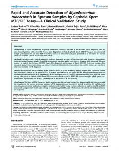
Fig. 2. SATé’s divide-and-conquer strategy, illustrated with a CT-2 decomposition. A branch in the initial tree is selected, and the subtrees—A, B, C, D—around the branch are determined. The sequences for each of the four subtrees are realigned by MAFFT. These realigned subproblems are then aligned with one another, two at a time, using Muscle, until an alignment on the full data set is obtained. RAxML then computes a tree on the alignment. SATé iterates this process, as shown in Fig. 1.
19 JUNE 2009
VOL 324
SCIENCE
www.sciencemag.org
Downloaded from www.sciencemag.org on September 11, 2009
phylogeny estimation methods (10). Still, estimation of phylogenies and alignments for large data sets is difficult and highly inaccurate when the sequences examined for phylogenetic reconstruction have evolved with many substitutions and insertions and deletions (indels). Alignment estimation methods typically estimate guide trees on which an alignment is then produced. The methods can be highly sensitive to the guide tree (3), and automated alignments often require manual realignment, sometimes necessitating months of intensive analysis of the sequences and taxa (11, 12). Manual realignment can be error prone due to limitations in alignment editors; the inability of an individual to view all the sequences simultaneously; or idiosyncratic, unstated realignment criteria. Also, hard-to-align DNA regions that might contain phylogenetically useful information may be rejected due to a lack of confidence in the alignments. Finally, regions that are hard to align are typically aligned differently by different programs, and phylogenies estimated on these different alignments can differ substantially (13). Consequently, molecular phylogenies often are produced using slowly evolving DNA regions that can be aligned relatively easily. Restriction to such regions likely has resulted in less fully resolved evolutionary histories for many groups due to underutilization of data. Current methods for estimating trees directly from unaligned sequences include POY (14), POY* (15), ALIFRITZ (16), BAli-Phy (17), and the method of Lunter et al. (18), while SATCHMO (19) can be used for estimating trees directly from amino acid sequences. These methods potentially circumvent some of the aforementioned issues, but have limitations of their own. POY and POY* can be run on large data sets but have not produced trees more accurate than those of the best twophase methods (15, 20). The other methods are based on parametric statistical models of sequence evolution including substitutions and indels. ALIFRITZ and BAli-Phy use models that allow multinucleotide indel events, engendering large computational burdens. A study assessing their performance (21) found that ALIFRITZ could analyze ~30 sequences, and BAli-Phy was limited to 10. Our studies of these methods on 100 taxon data sets (tables S28 and S29) showed that after 2 weeks of analysis, although BAli-Phy and ALIFRITZ were able to produce trees and alignments on some data sets, their trees were not as accurate as those produced by the best two-phase methods. A method that includes only singlenucleotide indel events (18) was reported to analyze data sets with 50 sequences (21); however, our attempts to test this method (fig. S4) revealed that the current implementation is not operational.
run are compared, and the one with the best ML score is returned. For a CT-i decomposition, SATé computes a bifurcating tree with maximum diameter 2i − 1 around a branch selected in the current best tree. The branch is typically either a midpoint branch (the middle branch on a longest path in the tree) or a centroid branch, which splits the tree into two subtrees with roughly equal numbers of taxa. A CT-i decomposition produces at most 2i subsets, which are clades in the current tree (see Fig. 2 and Supporting Online Material for examples), where i is user-specified (default: i = 5), allowing the number and size
an ML tree (general time reversible + gamma model) with RAxML. The “second stage” then uses an iterative, greedy search heuristic to find tree/alignment pairs with better ML scores (Fig. 1). In each iteration, a new alignment is proposed by our divide-and-conquer method: Center-Tree-i (CT-i) decomposition (Fig. 2). The default setting runs stage 2 for 24 hours, allowing the final iteration begun before the 24-hour limit to complete. The user can specify the stopping criterion, e.g., time limits or until no improvement in the ML score has occurred for 24 hours. If two or more starting tree/alignment pairs are used, the final tree/alignment pairs from each 0.5
Missing Branch Rate
0.4 0.3
RAxML(ClustalW) RAxML(Muscle) RAxML(MAFFT) RAxML(Prank+GT) SATé24 RAxML(TrueAln)
0.2 0.1 0
1
Alignment SP−FN Error
0.9 0.8 0.7 0.6
10
00 S5
10
00
L4
10
00 M4
10 00
M5
10 00
L5
10 00
10
10
10
S4
00
M3
10
00
S3 *
10 00
S2 *
10 00
M2 *
10 00
L2 *
10 00
L1
*
10 0
0L 3*
10
10 00 00 S1 M1 * *
ClustalW Muscle MAFFT Prank+GT SATé24
0.5 0.4 0.3 0.2 0.1 0
10
00 S
5
1
Setwise TrueAln Statistic
0.9 0.8
10 00 L
4
10
00 M
10 4
10
00 M
5
00 L
5
00 S4
00 M
10 3
00 S3
10 00
S2 *
10 00
M2 *
10
00 L
2
10
00 L
1*
10 0
0L
3
10 00
S1
10 0
0M
1
Percent indels Avg p−dist
0.7 0.6 0.5 0.4 0.3 0.2 0.1 0
10 00
S5
10
00
L4
10
00 M
10
00 M5
4
10 00
L5
10
00 S4
10
00 M3
10
00 S
3
10 00
S2
10 00
M2
10 00
L2
10 00
L1
10 00
L3
10 0
0S 1
10 0
0M 1
1 0.9 0.8 0.7
ρ
0.6 0.5 0.4 0.3 0.2
Norm. likelihood vs. missing branch rate Norm. likelihood vs. align. SP−FN error
0.1 0
10 0
0S
5
10 0
0L 4
10
00
M4
10
00 M5
10 00
L5
10
00 S4
10
00 M3
10
00 S3
10 00
S2
10 10 10 10 10 10 00 00 00 00 00 00 L1 S1 M1 L2 L3 M2
Fig. 3. The 1000-taxon model results. All x axes show the 15 1000-taxon models, from easy to hard, based on missing branch rates. From top-to-bottom panels, the y axes are missing branch rate, alignment SP-FN error, true alignment setwise statistics, and Spearman rank correlation coefficients (r). All data points include SE bars. For the top two panels, models on the x axis followed by an asterisk indicate that SATé’s performance was significantly better than the nearest two-phase method (paired t tests, setwise a = 0.05, n = 40 for each test). www.sciencemag.org
SCIENCE
VOL 324
of subproblems to be tuned for the number of taxa in the full data set. Sequences in each subset are realigned (default = MAFFT), and the alignments are progressively merged (default = Muscle), using the current tree as a guide tree, into an alignment on the full data set. An ML tree is estimated on the new alignment with RAxML. The tree/alignment pair with the better ML score (either the original pair or the new pair) is then used for the next iteration. To determine the best defaults and options for SATé, we explored multiple combinations of the algorithmic parameters (22). We observed that CT-5 decompositions performed reliably well, and that starting with a tree/alignment pair having a good ML score improved SATé’s convergence rate, but that SATé was robust to the choice of starting alignment/tree pairs (figs. S7 to S10 and tables S20, S21, and S28). Two variants of SATé performed particularly well. The first, SATé24, was fast and produced highly accurate alignments and trees. For its starting alignment/tree pair, SATé24 selects among four tree/alignment pairs by running RAxML on four alignments [ClustalW (23), Muscle, MAFFT, and Prank+GT, which is Prank provided with a RAxML-on-MAFFT guide tree] and picks the pair with the best ML score on its tree. SATé24 then uses its hill-climbing strategy for 24 hours to search for better solutions. The second variant, SATéBML, was slower but produced more accurate alignments and trees than the first. It uses two starting alignment/tree pairs (the ClustalW alignment and its RAxML tree, and the pair used by SATé24), lets each of the hill-climbing SATé analyses run until no change has occurred for 24 hours, and returns the solution with the best ML score. We tested these SATé variants on both simulated and biological data sets, relative to the alignment methods ClustalW, MAFFT, Muscle, and Prank+GT, and to RAxML, run to completion. For the simulation studies, we compared SATé24 to the two-phase methods, using ROSE (24) to simulate sequence evolution under 30 models (20 replicates per model, root sequences of 1000 base pairs, trees of 500 and 1000 taxa) representing a wide range of conditions (tables S1 to S3). We used ROSE’s output to determine the true alignment for each data set and the model-tree branches on which no changes occurred (zero-event branches). We used the true alignment to calculate SP-FN alignment error rates. SP-FN is the sum of pairs for the false-negative error rate: the percentage of evolutionarily homologous pairs of nucleotides missing in the estimated alignment and the complement of the SP accuracy measure (25). We contracted zero-event branches of the model trees—because reconstruction of these branches is effectively random (26)—producing potentially inferable model trees (PIMTs). We used the PIMTs to quantify the percentage of branches missing from an estimated tree but present in the PIMT (the missing branch rate). RAxML runs on the true alignment consistently produced a low proportion of missing branches
19 JUNE 2009
Downloaded from www.sciencemag.org on September 11, 2009
REPORTS
1563
REPORTS Because tree error may increase when unreliable sites are included, we estimated ML trees on data sets from which sites were eliminated using four techniques [including two variants of Gblocks (27)]. These techniques either had little impact on tree estimation accuracy or made the estimations worse (tables S31 to S34). SATé24’s improved tree/alignment accuracy arose from its divide-and-conquer strategy and use of the ML criterion. The CT-5 decomposition improved starting alignments and trees on the moderate-to-difficult models (table S11) and modified (without necessarily improving) them on the easy models (table S12). The ML score was positively correlated with alignment and tree accuracy across all models, especially the moderateto-difficult models (Fig. 3, fig. S6, and tables S14 and S15). Furthermore, even when SATé24 proposed alignments that were accepted but resulted in trees of reduced accuracy, the average reduction in alignment or tree accuracy was at most 0.5% (table S11). SATé sometimes found better trees and alignments with different starting tree/alignment pairs (figs. S7 and S9 and table S28). Therefore, we recommend multiple runs of SATé using more than one starting pair, e.g., using SATéBML if time permits. We compared SATéBML to the two-phase methods on six biological ribosomal RNA data sets (117 to 1028 taxa; table S7) for which highly reliable, curated alignments are available. SATéBML and MAFFT alignments were of comparable accuracy and better than the other alignments (table S18), and SATéBML trees were more accurate than those produced by any two-phase method (table S19). Thus, SATé is a fast, effective, and fully automated method for simultaneous estimation of trees and alignments for nucleotide sequences on large numbers of taxa. For rapidly evolving sequences, it dramatically speeds and improves tree and alignment estimations compared to the best current two-
Table 1. Missing branch rates and alignment SP-FN error rates. For each statistic and model, the bestperforming methods (within 1%) are in boldface. The best overall is indicated with an asterisk (*). For each “All models” entry, n = 600; for each easy entry, n = 120; for each moderate-to-difficult entry, n = 180.
1564
Method
All models % (SE)
RAxML(TrueAln) SATé RAxML(Prank+GT) RAxML(MAFFT) RAxML(Muscle) RAxML(ClustalW)
7.4 (0.1) *9.1 (0.2) 13.0 (0.3) 12.6 (0.4) 15.3 (0.5) 21.6 (0.6)
SATé Prank+GT MAFFT Muscle ClustalW
*14.2 18.5 20.6 22.7 46.9
(0.6) (0.8) (0.8) (0.9) (1.3)
Moderate to difficult
1000 % (SE)
500 % (SE)
Missing branch rate 9.3 (0.1) 8.4 (0.1) *13.1 (0.3) *10.4 (0.2) 21.0 (0.6) 15.2 (0.4) 21.6 (0.6) 13.5 (0.3) 22.9 (1.0) 20.5 (0.9) 38.7 (0.7) 21.6 (0.6) Alignment SP-FN error rate *25.0 (1.3) *21.3 (0.7) 30.6 (1.2) 29.9 (1.1) 38.6 (1.3) 28.5 (1.0) 34.0 (1.4) 38.5 (1.5) 77.1 (1.1) 64.1 (1.2)
19 JUNE 2009
VOL 324
1000 % (SE)
Easy
500 % (SE)
5.1 (0.1) *5.1 (0.1) *5.1 (0.1) *5.1 (0.1) 5.4 (0.1) 5.3 (0.1)
5.3 5.4 *5.3 *5.3 5.8 5.7
*0.4 (0.02) *0.4 (0.02) 0.9 (0.1) 1.8 (0.1) 9.8 (0.5)
*1.0 (0.1) 1.1 (0.1) 1.7 (0.1) 2.9 (0.2) 12.9 (0.6)
SCIENCE
(0.1) (0.1) (0.1) (0.1) (0.1) (0.1)
phase methods, and it removes or significantly reduces the need for hand realignment of data sets. Finally, it makes possible the use of DNA regions previously rejected for alignment difficulty, potentially leading to significantly improved resolution of species’ relationships. References and Notes
1. K. Katoh, K. Kuma, H. Toh, T. Miyata, Nucleic Acids Res. 33, 511 (2005). 2. C. B. Do, M. Mahabhashyam, M. Brudno, S. Batzoglou, Genome Res. 15, 330 (2005). 3. S. Nelesen, K. Liu, D. Zhao, C. R. Linder, T. Warnow, Pac. Symp. Biocomput. 13, 25 (2008). 4. A. Loytynoja, N. Goldman, Proc. Natl. Acad. Sci. U.S.A. 102, 10557 (2005). 5. R. C. Edgar, BMC Bioinformatics 5, 113 (2004). 6. R. C. Edgar, S. Batzoglou, Curr. Opin. Struct. Biol. 16, 368 (2006). 7. A. Stamatakis, Bioinformatics 22, 2688 (2006). 8. A. Stamatakis, in Proc. 20th IEEE International Parallel and Distributed Processing Symposium, Rhodes Island, Greece, 25 to 29 April 2006 (IEEE Computer Society, Los Alamitos, CA, 2006), pp. 278–285. 9. D. Zwickl, GARLI download page (2006); project Web site at www.zo.utexas.edu/faculty/antisense/Garli.html. 10. S. Guindon, O. Gascuel, Syst. Biol. 52, 696 (2003). 11. L. Goertzen, J. Cannone, R. Gutell, R. Jansen, Mol. Phylogenet. Evol. 29, 216 (2003). 12. Early Bird ATOL Project, (2007); project Web site at www. fieldmuseum.org/research_collections/zoology/zoo_sites/ early_bird/. 13. K. M. Wong, M. A. Suchard, J. P. Huelsenbeck, Science 319, 473 (2008). 14. A. Varón, L. S. Vinh, I. Bomash, W. C. Wheeler, POY Software (2007). Documentation by A. Varón et al. Available for download at research.amnh.org/scicomp/ projects/poy.php. 15. K. Liu, S. Nelesen, S. Raghavan, C. Linder, T. Warnow, IEEE/ACM Trans. Comput. Biol. Bioinform. 6, 7 (2009). 16. R. Fleissner, D. Metzler, A. von Haeseler, Syst. Biol. 54, 548 (2005). 17. B. D. Redelings, M. Suchard, Syst. Biol. 54, 401 (2005). 18. G. Lunter, I. Miklós, A. Drummond, J. L. Jensen, J. Hein, BMC Bioinformatics 6, 83 (2005). 19. R. C. Edgar, K. Sjolander, Bioinformatics 19, 1404 (2003). 20. T. Heath Ogden, M. S. Rosenberg, Syst. Biol. 55, 314 (2006). 21. G. Lunter, A. Drummond, I. Miklós, J. Hein, in Statistical Methods in Molecular Evolution (Statistics for Biology and Health), R. Nielsen, Ed. (Springer, Berlin, 2005), pp. 375–406. 22. Materials and methods are available as supporting materials on Science Online. 23. J. D. Thompson, D. Higgins, T. Gibson, Nucleic Acids Res. 22, 4673 (1994). 24. J. Stoye, D. Evers, F. Meyer, Bioinformatics 14, 157 (1998). 25. J. D. Thompson, F. Plewniak, O. Poch, Bioinformatics 15, 87 (1999). 26. R. Desper, O. Gascuel, Mol. Biol. Evol. 21, 587 (2004). 27. G. Talavera, J. Castresana, Syst. Biol. 56, 564 (2007). 28. This research was supported by the U.S. NSF under grants DEB 0733029, ITR 0331453, ITR 0121680, EIA 0303609, and IGERT 0114387. The simulated and biological data sets, true and curated alignments, PIMTs, and all software are available at www.cs.utexas.edu/users/ tandy/science-paper.html.
Supporting Online Material www.sciencemag.org/cgi/content/full/324/5934/1561/DC1 Materials and Methods SOM Text Figs. S1 to S10 Tables S1 to S34 References 22 January 2009; accepted 30 April 2009 10.1126/science.1171243
www.sciencemag.org
Downloaded from www.sciencemag.org on September 11, 2009
(averaging 7.4% overall), even when run on models whose true alignments contained high proportions of indels and high substitution rates (Fig. 3 and fig. S6), indicating that treating indels as missing data introduced minimal error in tree estimation, even for data sets containing many indels. SATé24’s missing branch rates (averaging 9.1% overall) were only somewhat higher than those obtained by RAxML on the true alignment (Table 1). By comparison, the overall average missing branch rates for RAxML trees produced on estimated alignments were 12.6% for MAFFT, 13.0% for Prank+GT, 15.3% for Muscle, and 21.6% for ClustalW (Table 1). On these data sets, runtimes for SATé24’s second stage were at most 28 hours for 500 taxa and 34 hours for 1000 taxa (table S9). We labeled some models “easy” because all methods produced trees with accuracy close to that of RAxML on the true alignment (Fig. 3 and fig. S6). For the remaining “moderate-to-difficult” models (Table 1, Fig. 3, and fig. S6), SATé24 produced the most accurate trees and alignments, ClustalW produced the least, and the other methods were intermediate. SATé24’s missing branch rates on the moderate-to-difficult models were significantly better than those produced by the closest two-phase method in all cases (P ≤ 0.004; paired t test) except that of model 1000M3, whose performance was similar to that obtained by running RAxML on a MAFFT alignment (Fig. 3 and table S13). For all methods, missing branch rates and alignment error rates tended to increase as the number of taxa (Table 1) or rate of evolution increased (Fig. 3); however, SATé24’s error rates generally increased much less than those of the other methods. Thus, SATé24 provided the largest advantage on the hardest data sets. SATé24’s worst average missing branch rate (17.4%) was on model 1000M1, on which all other methods had error rates >30% (Fig. 3). Furthermore, SATé24 achieved these performance gains on standard desktop computers with 4 GB of RAM.