Rapid Detection of Botnets through Collaborative ... - Computer Science

Rapid Detection of Botnets through Collaborative Networks of Peers

A thesis presented by David J. Malan to The School of Engineering and Applied Sciences in partial fulfillment of the requirements for the degree of Doctor of Philosophy in the subject of Computer Science Harvard University Cambridge, Massachusetts June 2007

c 2007 – David J. Malan °

All rights reserved.

Thesis advisor Michael D. Smith

Author David J. Malan

Rapid Detection of Botnets through Collaborative Networks of Peers

Abstract Botnets allow adversaries to wage attacks on unprecedented scales at unprecedented rates, motivation for which is no longer just malice but profits instead. The longer botnets go undetected, the higher those profits. I present in this thesis an architecture that leverages collaborative networks of peers in order to detect bots across the same. Not only is this architecture both automated and rapid, it is also high in true positives and low in false positives. Moreover, it accepts as realities insecurities in today’s systems, tolerating bugs, complexity, monocultures, and interconnectivity alike. This architecture embodies my own definition of anomalous behavior: I say a system’s behavior is anomalous if it correlates all too well with other networked, but otherwise independent, systems’ behavior. I provide empirical validation that collaborative detection of bots can indeed work. I validate my ideas in both simulation and the wild. Through simulations with traces of 9 variants of worms and 25 non-worms, I find that two peers, upon exchanging summaries of system calls recently executed, can decide that they are, more likely than not, both executing the same worm as often as 97% of the time. I deploy an actual prototype of my architecture to a network of 29 systems with which I monitor and analyze 10,776 processes, inclusive of 511 unique non-worms (873 if unique versions constitute unique non-worms). Using that data, I expose the utility of temporal consistency (similarity over time in worms’ and non-worms’ invocations of system calls) in collaborative detection. I identify properties with which to distinguish non-worms from worms 99% of the time. I find that a collaborative network, using patterns of system calls and simple heuristics, can detect worms running on multiple hosts. And I find that collaboration among peers significantly reduces the risk of false positives because of the unlikely, simultaneous appearance across peers of non-worm processes with worm-like properties.

Contents . . . . . . . .

i iii iv vi vii viii ix x

. . . . . .

1 3 6 7 7 10 13

. . . . . . . . .

15 15 16 19 19 23 25 28 29 31

3 True Positives 3.1 Questions . . . . . . . . . . . . . . . . . . . . . . . . . . . . . . . . . 3.2 Methodology . . . . . . . . . . . . . . . . . . . . . . . . . . . . . . .

33 36 37

Title Page . . . . . . Abstract . . . . . . . Table of Contents . . List of Figures . . . . List of Tables . . . . Citations to Previous Acknowledgments . . Dedication . . . . . .

. . . . . . . . . . . . . . . . . . . . . . . . . . . . . . . . . . . . . . . . Publications . . . . . . . . . . . . . . . .

. . . . . . . .

. . . . . . . .

1 Introduction 1.1 Why Security Is Hard . . . . . . . 1.2 Detection of Botnets . . . . . . . 1.3 From Botnets to Worms . . . . . 1.3.1 How Not to Detect Worms 1.3.2 How to Detect Worms . . 1.4 Contributions . . . . . . . . . . .

. . . . . . . . . . . . . .

. . . . . . . . . . . . . .

. . . . . . . . . . . . . .

. . . . . . . . . . . . . .

. . . . . . . . . . . . . .

. . . . . . . . . . . . . .

. . . . . . . . . . . . . .

. . . . . . . . . . . . . .

. . . . . . . . . . . . . .

. . . . . . . . . . . . . .

. . . . . . . . . . . . . .

. . . . . . . . . . . . . .

2 Host-Based, Collaborative Detection of Worms 2.1 Anomalous Behavior of Worms . . . . . . . . . . . . . 2.2 A Behavior-Based, Distributed IDS . . . . . . . . . . . 2.3 Temporal Consistency . . . . . . . . . . . . . . . . . . 2.3.1 System Calls as a Proxy for Behavior . . . . . . 2.3.2 Measuring Similarity with Levenshtein Distance 2.3.3 Measuring Similarity with Intersection . . . . . 2.4 Related Work . . . . . . . . . . . . . . . . . . . . . . . 2.5 Discussion of Threats . . . . . . . . . . . . . . . . . . . 2.6 Summary . . . . . . . . . . . . . . . . . . . . . . . . .

iv

. . . . . . . . . . . . . . . . . . . . . . .

. . . . . . . . . . . . . . . . . . . . . . .

. . . . . . . . . . . . . . . . . . . . . . .

. . . . . . . . . . . . . . . . . . . . . . .

. . . . . . . . . . . . . . . . . . . . . . .

. . . . . . . . . . . . . . . . . . . . . . .

. . . . . . . . . . . . . . . . . . . . . . .

Contents

3.3

3.4

v

3.2.1 Wormboy 1.0 . . . . . . . . . . . . . . . . . . 3.2.2 Traces of Worms and Non-Worms . . . . . . . Results . . . . . . . . . . . . . . . . . . . . . . . . . . 3.3.1 How likely is a worm to look like itself? . . . . 3.3.2 How likely is a non-worm to look like itself? . 3.3.3 How likely is a non-worm to look like a worm? Summary . . . . . . . . . . . . . . . . . . . . . . . .

4 False Positives 4.1 Questions . . . . . . . . . . . . . . . . . . 4.2 Methodology . . . . . . . . . . . . . . . . 4.2.1 Wormboy 2.0: Peers’ Client . . . . 4.2.2 Wormboy 2.0: The Snapshot Server 4.3 Results . . . . . . . . . . . . . . . . . . . . 4.3.1 Identifying τ , r, and r0 . . . . . . . 4.3.2 Detecting Processes across Peers . . 4.3.3 Avoiding False Positives . . . . . . 4.4 Summary . . . . . . . . . . . . . . . . . . 5 Scalability 5.1 Framework for Assessment . . . . . . . . . 5.2 Self-Monitoring By Peers . . . . . . . . . . 5.3 Submission of Snapshots . . . . . . . . . . 5.4 Analysis of Snapshots . . . . . . . . . . . . 5.4.1 Pairwise Comparison of Snapshots 5.4.2 Searching for Cliques . . . . . . . . 5.5 Summary . . . . . . . . . . . . . . . . . .

. . . . . . . . . . . . . . . .

. . . . . . . . . . . . . . . .

. . . . . . . . . . . . . . . .

. . . . . . . . . . . . . . . .

. . . . . . . . . . . . . . . .

. . . . . . . . . . . . . . . .

. . . . . . . . . . . . . . . . . . . . . . .

. . . . . . . . . . . . . . . . . . . . . . .

. . . . . . . . . . . . . . . . . . . . . . .

. . . . . . . . . . . . . . . . . . . . . . .

. . . . . . . . . . . . . . . . . . . . . . .

. . . . . . . . . . . . . . . . . . . . . . .

. . . . . . . . . . . . . . . . . . . . . . .

. . . . . . . . . . . . . . . . . . . . . . .

. . . . . . .

38 39 40 40 43 45 46

. . . . . . . . .

49 50 51 52 53 54 54 57 61 63

. . . . . . .

67 67 68 70 75 75 78 82

6 Conclusions and Future Work

85

Bibliography

88

List of Figures 1.1

A false positive typical of behavior-based IDSes . . . . . . . . . . . .

2.1 2.2 2.3 2.4

My vision of collaborative detection . . . . . . . . . . . . . . . . Hypothetical trace of a . . . process’s invocation of . . . system calls Application of Levenshtein distance to a pair of snapshots . . . Application of intersection to a pair of snapshots . . . . . . . . .

3.1 3.2 3.3 3.4 3.5 3.6 3.7

Traces of one host’s behavior . . . . . . . . . Calls to system services by Worm/Lovesan.A Calls to system services by I-Worm/Sasser.B Calls to system services by I-Worm/Bagle.Q Calls to system services by Worm/Lovesan.H Calls to system services by Worm/Lovesan.H Degrees, τ , of temporal consistency of worms

4.1 4.2 4.3 4.4 4.5

Wormboy 2.0’s definition of a snapshot . . . . . . . . . . τ versus r versus r0 for worms and non-worms . . . . . . Rates of recognition of non-worms . . . . . . . . . . . . . Average and maximal rates of recognition for non-worms Snapshots from sshd.exe and I-Worm/Mydoom.F . . .

. . . . .

. . . . .

5.1 5.2 5.3 5.4 5.5 5.6 5.7

Sizes of snapshots . . . . . . . . . . . . . . . . . . . . . . . . . . Distribution of system services . . . . . . . . . . . . . . . . . . . Implementation of snapshots’ comparison . . . . . . . . . . . . . Implementation of 1-bit counting . . . . . . . . . . . . . . . . . Time required for centralized analysis of snapshots for similarity Probabilities of edges among peers . . . . . . . . . . . . . . . . Time required for discovery of maximal cliques . . . . . . . . . .

. . . . . . .

vi

. . . .

. . . .

17 21 24 27

. . . . . . . . . . . . . . . . . . . . . . . . . . . . . . . . . . . . . . . . . . . . . . . . . . . . per 5-second window . per 15-second window versus non-worms . .

. . . . . . .

35 42 43 44 46 47 48

. . . . .

. . . . .

53 58 59 61 66

. . . . . . .

. . . . . . .

73 77 78 79 80 83 84

. . . . .

. . . . .

. . . . .

. . . .

9

List of Tables 3.1 3.2 3.3

Worms and non-worms whose traces I analyzed . . . . . . . . . . . . Probability . . . using Levenshtein distance . . . . . . . . . . . . . . . . Probability . . . using intersection . . . . . . . . . . . . . . . . . . . . .

40 41 45

4.1 4.2 4.3

Nineteen non-worms that exhibit worm-like behavior . . . . . . . . . Results of . . . examination of 10,776 non-worm processes . . . . . . . Similarity over time of 14 worm-like non-worms . . . . . . . . . . . .

56 57 65

5.1 5.2 5.3 5.4

Results of executing PC World’s WorldBench 5 Snapshots per window per host . . . . . . . . . Sizes of snapshots . . . . . . . . . . . . . . . . . Estimates . . . for transmission of . . . snapshots .

69 72 74 74

vii

. . . .

. . . .

. . . .

. . . .

. . . .

. . . .

. . . .

. . . .

. . . .

. . . .

. . . .

. . . .

Citations to Previous Publications Portions of this thesis are adapted or excerpted from these publications. David J. Malan and Michael D. Smith. “Host-Based Detection of Worms through Peer-to-Peer Cooperation.” ACM Workshop on Rapid Malcode. Fairfax, Virginia. November 2005. David J. Malan and Michael D. Smith. “Exploiting Temporal Consistency to Reduce False Positives in Host-Based, Collaborative Detection of Worms.” ACM Workshop on Recurring Malcode. Fairfax, Virginia. November 2006.

Acknowledgments My thanks to John Dias, Paul Govereau, Kelly Heffner, Glenn Holloway, Kevin Redwine, and David van Dyk for their support throughout this work. My thanks to Wellie Chao, Rei Diaz, Anthony DiComo, Breanne Duncan, Kathleen Durant, Kelly Heffner, Glenn Holloway, Matthew Fluet, Matthew Foroughi, Dianne Malan, Lauren Malan, Tomas Mikuckis, Gordon Murphy, Daniel Peng, Chris Power, Roman Rubinstein, Andrew Smith, Samantha Smith, Shane Smith, Lifan Yang, and Xin-Xin Zeng for welcoming Wormboy into their kernels for this work. My thanks to Michael Mitzenmacher and Greg Morrisett for their counsel on this work. And my thanks and gratitude to Michael D. Smith, without whom this work would not exist.

dedicated to Henry H. Leitner

Chapter 1 Introduction Botnets are networks of systems on which adversaries have somehow installed software called bots that they can remotely control, typically unbeknownst to those systems’ own owners [10, 62, 70]. For all intents and purposes, bots are just viruses or worms that happen to allow remote command and control [22, 32] by adversaries. The value of botnets to adversaries derives from their size. Not only do they provide adversaries with cycles and bandwidth for which they need not pay, they allow adversaries to wage attacks on unprecedented scales at unprecedented rates. Large numbers of bots are of particular value these days for distributed denial-of-service (DDoS) attacks [43, 74, 82], relay of spam [63], and click fraud [22]. Botnets exist because we are not very good at keeping our systems secure. Few days seem to go by without some announcement of newly discovered vulnerabilities in some software-based product or service, many of them “critical.” According to Microsoft, the #3 reason (out of 100) to purchase Windows Vista is that it’s “the safest version of Windows ever” [50]. However, it’s about Windows Vista that some of those announcements have been [12–15]. Not just botnets but also viruses, worms, and spyware seem to have entered the general lexicon, testament to their ubiquity. 1

Chapter 1: Introduction

2

Of course, users might still have trouble distinguishing each of those threats, but they certainly seem to be worried about them nonetheless. Rightly so, if nearly 90% of their computers are already infected with some form thereof [89]. To be sure, we, as users, do install anti-this and anti-that. And today’s operating systems do tend to update themselves automatically. But clearly our adversaries are still slipping past our defenses. We just make it so easy to do so. We continue to write buggy software, and it’s in bugs that adversaries typically find opportunities for malice. We write increasingly complex software, which typically means more bugs and, thus, more opportunities. We also all run the same software, and it’s in monocultures that adversaries find identical opportunities. Of course, we might not be much better at security in the real world. After all, banks are still robbed and homes are still burgled. But this Internet of ours seems to exacerbate weaknesses that, in the physical world, are mitigated by distance and time. In the physical world, banks and homes simply are not within reach of all possible adversaries. In the physical world, adversaries simply cannot attack all possible banks and all possible homes in just minutes or seconds. The combination of bugs, complexity, and monocultures with such extreme interconnectivity certainly means trouble. In the words of Hoglund and McGraw [31], connectivity and complexity alone constitute two pillars of a “trinity of trouble.”1 I say trouble because these realities present opportunities not only for malice but also for profit. Merely crashing systems, perhaps once upon a time interesting, is not particularly profitable. Far more alluring to adversaries is monetization of our insecurities. Those “critical” bugs, after all, allow black hats to install their 1

The extensibility of today’s systems is McGraw’s third pillar.


3

own software and take control of our systems, often without our knowledge. With access to the cycles and bandwidth of hundreds or thousands or millions of systems, adversaries can wage (or sell) any number of attacks [72]. Thus do we have botnets. In time, new tools and languages may very well help us write code that, while still complex, nonetheless suffers fewer bugs per line. But bugs and complexity are probably with us for some time. As for our monocultures, we could diversify our systems but only to limited extent. After all, choices (of, say, operating systems) and resources (to, say, support them) are limited. The challenge, then, is to live with bugs, to live with complexity, to live with monocultures. The challenge is to live with systems like ours on today’s Internet but do better than we are currently doing with regard to security, even though it is hard. This thesis shows that we can. We might not be very good at keeping adversaries, and thus bots, off of our systems. But I claim that we can detect them rapidly when they are there.

1.1

Why Security Is Hard

A system that is “powered off, cast in a block of concrete, and sealed in a lead-lined room with armed guards” [80] might be secure, but it certainly isn’t useful. And so we take it out and power it on. We network it with other systems and then network those networks. The net result is, of course, our Internet, the transitive closure of which is a scary place. Much unlike our physical world, in which oceans and land keep adversaries at bay, this Internet puts each system quite within reach of every other, any one of which might prove a threat.


4

We thus guard our systems with software, typically layers of software so that we have “defense in depth” [53]. We erect firewalls. We brew honeypots. We install intrusion-detection systems. We deploy virus scanners. And we ready other defenses still. We occupy, after all, the so-called “position of the interior” [73]. Whereas we must find and fill all holes in our systems, our adversaries need find and exploit just one in the same. And it’s certainly easier to find one than all. Statistics are on our adversaries’ side. Anderson [6] paints the situation as follows. . . . suppose a large, complex product such as Windows 2000 has 1,000,000 bugs, each with a MTBF2 of 1,000,000,000 hours. Suppose that Paddy works for the Irish Republican Army, and his job is to break into the British Army’s computer to get the list of informers in Belfast; while Brian is the army assurance guy whose job is to stop Paddy. So he must learn of the bugs before Paddy does. Paddy has a day job so he can only do 1000 hours of testing a year. Brian has full Windows source code, dozens of PhDs, control of the commercial evaluation labs, an inside track on CERT, an information sharing deal with other UKUSA member states—and he also runs the government’s scheme to send round consultants to critical industries such as power and telecomms to advise them how to protect their systems. Suppose that Brian benefits from 10,000,000 hours a year worth of testing. After a year, Paddy finds a bug, while Brian has found 100,000. But the probability that Brian has found Paddy’s bug is only 10%. After ten years he will find it—but by then Paddy will have found nine more, and it’s unlikely that Brian will know all of them. Worse, Brian’s bug reports will have become such a firehose that Microsoft will have killfiled him. In other words, Paddy has thermodynamics on his side. Even a very moderately resourced attacker can break anything that’s at all large and complex. There is nothing that can be done to stop this, so long as there are enough different security vulnerabilities to do statistics: different testers find different bugs. (The actual statistics are somewhat more complicated, involving lots of exponential sums; keen readers can find the details [in Brady et al. [11]].) 2

mean time between failures


5

If we accept that our adversaries have this constant advantage, this is, as they say, a losing battle. Even though there are, according to Anderson, “various ways in which one might hope to escape this statistical trap.” First, although it’s reasonable to expect a 35,000,000 line program like Windows 2000 to have 1,000,000 bugs, perhaps only 1% of them are security-critical. This changes the game slightly, but not much; Paddy now needs to recruit 100 volunteers to help him (or, more realistically, swap information in a grey market with other subversive elements). Still, the effort required of the attacker is still much less than that needed for effective defense. Second, there may be a single fix for a large number of the security critical bugs. For example, if half of them are stack overflows, then perhaps these can all be removed by a new compiler. Third, you can make the security critical part of the system small enough that the bugs can be found. This was understood, in an empirical way, by the early 1970s. However, the discussion in the above section should have made clear that a minimal TCB3 is unlikely to be available anytime soon, as it would make applications harder to develop and thus impair the platform vendors’ appeal to developers. “Attack is simply easier than defense,” admits Anderson, at least when it comes to real-world systems. In the world of cryptography, we tend to enjoy quite the opposite relationship with our adversaries. Consider a cryptosystem based on two functions, Enc and Dec, and the secrecy of some key, k, whereby Deck (Enck (m)) = m, where m is some plaintext. To compromise this cryptosystem via brute force, an adversary must, on average, try 2|k|−1 possible keys. That is, given c = Enck (m), an adversary must compute Deck (c) for 2|k|−1 values of k on average. Assuming an adversary of limited computational resources (i.e., polynomially equivalent to our own), a onebit increase in the the size of k therefore doubles the adversary’s running time while, typically, increasing our own (i.e., that of Enc and Dec) only linearly. In other words, 3

trusted computing base


6

that which is linear in cost for us is exponential in cost for our adversary. More to the point, in this world of cryptography, we have it easier than our adversary. When it comes to real-world systems, though, we enjoy no such imbalance. Rather, it’s we who must keep up with our adversaries. We might very well have some defenses in place for our systems. But each time our adversaries discover means for circumvention thereof, we must scramble to patch the new leak. And it’s never long before adversaries spring the next. Security is hard because this playing field is not level.

1.2

Detection of Botnets

Detection of botnets is not easy. After all, their traffic (e.g., SMTP or HTTP) tends to resemble that of systems not under adversaries’ control. Spam is just email. And fraudulent clicks are still clicks. Moreover, victims of botnets’ attacks experience those attacks from all different directions (i.e., many different IP addresses). How to distinguish customers from bots is not necessarily obvious when it’s some virtual store that’s under attack. But the longer a botnet goes undetected, the more profits our adversaries might gain. The longer a botnet goes undetected, the more cycles and bandwidth (and sales) we might lose. Detect botnets quickly, though, and we might lower those profits. Detect botnets quickly, and we might render our systems, despite all their flaws, far less attractive to adversaries. To be sure, an adversary’s profits also tend to grow with a botnet’s size. The more bots an adversary controls, the more attacks he can wage. We might therefore


7

render botnets less profitable by combatting their size. I focus in this thesis, though, on time to detection rather than size. After all, the sooner we detect a botnet at all, the sooner we can impede further growth thereof.

1.3

From Botnets to Worms

Detection of botnets reduces to detection of bots across systems. In different forms do these bots come, but I focus on worms for this thesis. Unlike viruses, which require action by humans to propagate, worms travel and execute across systems all by themselves. And they move quickly. Worms’ rates of propagation are no longer measured in hours but in minutes [51, 65, 91]. So fast are the fastest that human intervention no longer is possible [81, 82]. Detection must therefore be automated like the adversaries themselves. But with automation comes a risk of false positives, whereby benign applications (non-worms) might be misclassified as worms. The question at hand, then, is whether we can build intrusion-detection systems (IDSes) that are not only automated and rapid but also high in true positives and low in false positives.

1.3.1

How Not to Detect Worms

Common today are IDSes based on automated recognition of signatures, sequences of bytes indicating some worm’s presence in memory or network traffic. Such defenses are fast, and specificity of signatures renders false positives unlikely. But the protections are limited: systems are safe from only those worms for which researchers have had time to craft signatures, and signature-based defenses can be defeated by


8

metamorphic or polymorphic worms [38, 90]. Signatures require that we constantly “dance” with our adversary: for each change that he makes to his worm to avoid detection, we must respond manually with a step of our own. Behavior-based defenses offer an attractive alternative. Not only are they effectively automated, they try to stay one step ahead of our adversaries by monitoring systems for anomalous (e.g., yet unseen) behavior. Moreover, they are perhaps less susceptible to defeat by mere transformations of text, insofar as they judge the effect of code more than they do its appearance. But this resilience comes at a cost: accuracy or usability. Faced with some anomalous action, behavior-based defenses must either block that action, potentially impeding desired behavior, or wait for the user’s judgement. Such defenses can therefore be defeated by users themselves if annoyed or confounded by too prompts. Figure 1.1 presents one such nuisance. If threats are judged non-threats, the results are infections. If non-threats are judged threats, the results are false positives. Consequently, defenses as high in false positives as they are in true positives are perhaps just as bad as no defenses at all. Both put systems’ usability at risk. Inherent in IDSes, then, are “virtual knobs.” Settings tailored to known worms’ behaviors tend to produce few false positives but are easier for worms’ authors to circumvent in future designs. Settings that detect many behaviors (and thus many worms), meanwhile, tend to produce many false positives. The ideal IDS detects many behaviors without producing false positives. Today’s IDSes, of course, are far from ideal. Not only do they suffer false positives, they also suffer false negatives, whereby actual worms are not detected at all. Examples abound; I offer just two for


9

Figure 1.1: A false positive typical of behavior-based IDSes that monitor systems for worrisome (e.g., previously unseen) activity. In this particular instance, an attempt to modify the Windows registry by QuickTime [8] is flagged by Spybot [39] as anomalous behavior. The user is thus prompted to approve or deny the change even though it does not constitute an actual threat. Behavior-based defenses tend to “cry wolf” in this manner so often that they are vulnerable to defeat by users themselves if annoyed or confounded by too many prompts. the sake of discussion. In April 2004, we experienced Sasser (also known as Jobaka), a worm that compels certain versions of Windows to shut down. Even those systems with Norton AntiVirus already installed were not safe until Symantec released “virus definitions, version 30/04/04 rev 70 (20040430.070)” [88]. Earlier in 2004 had we already experienced Bagle, a mass-mailing worm. According to Symantec, “Beta definitions 27975, dated February 17, 2004, 5:20AM PT, or later will detect this threat” [85]. These anecdotes are only to say that Norton AntiVirus failed to detect both Bagle and Sasser upon their release. To be fair, Symantec’s competition did not fare any better. McAfee also raced to update its own software upon these worms’


10

discovery [46, 49]. Similarly did Lovesan (otherwise known as Blaster) [47, 86] and Mydoom [48, 87] go undetected, along with many other worms, until both vendors updated their products. That such vendors as these update their products’ so-called “definitions” continually (i.e., daily or weekly) is itself evidence that worms quite often go undetected by customers’ systems until their defenses are updated. I again claim that we can do better. The architecture that I herein propose offers to detect such worms as these without this inherent need for continual updates.

1.3.2

How to Detect Worms

Rather than focus on adjustment of knobs, I propose a new take on anomalous behavior altogether. Conventional behavior-based defenses dictate that hosts evaluate some current action vis-à-vis prior actions or blacklisted actions. A host’s behavior is deemed anomalous if it differs from that host’s prior behavior or resembles activity deemed worrisome a priori by some authority (e.g., McAfee [45] or Symantec [84]). The implication, though, is that a host’s behavior might be deemed anomalous simply because: • some process followed a new, but benign, code path for the first time; • some new, but benign, application is installed for which the host has no history of behavior; or • some process behaves in a way that might be, but isn’t necessarily, worrisome (as in Figure 1.1).


11

In none of these situations do users want prompts, let alone false positives. These defenses are limited, then, by their own design. Periodic updates of blacklists (or signatures) aside, today’s defenses operate largely in isolation, focusing more on the security of one system rather than on that system plus others like it. These defenses fail to consider all available information. When in doubt as to the nature of some process, systems tend not to consult each other for “advice,” hints as to whether some behavior is indeed worthy of concern. By definition, though, worms do not execute on systems one at a time. I claim, then, that if multiple systems suddenly share some concern (i.e., within some window of just a few seconds), that in itself is an additional hint that some behavior might belong to a worm. I thus offer an alternative definition of anomalous behavior. I propose that a host evaluate some current action vis-à-vis its peers’ current actions; a host’s behavior should be deemed anomalous if it correlates all too well with other, otherwise independent, hosts’ behavior. To be sure, this definition immediately puts the behavior of distributed applications and popular applications (that are running across many systems at once) at risk of being classified as anomalous. But I do not claim that this approach should be used instead of all others. It can certainly complement more traditional techniques. Moreover, we could tolerate coordinated behavior in distributed applications (e.g., Entropia [16]) and even popular applications by maintaining whitelists for software known not to be worms, as with read-only hashes of benign executables. (Some distributed applications already provide protections in their virtual machines against ill-behaved and malicious grid programs anyway.) However, my focus in this thesis is on more generalized techniques than these.


12

I thus present in this thesis the design for an IDS that detects this distributed form of anomalous behavior. I show that, by leveraging collaboration among internetworked peers, we can achieve high rates of true positives and low rates of false positives. Worms can be distinguished from non-worms by their simplicity and periodicity: their design is to spread, and their execution is cyclical. Of course, even non-worms can manifest cyclical behavior reminiscent of worms’, but I claim that we are less likely to see such behavior simultaneously on networked, but otherwise independent, hosts, unless it’s on purpose. Worms’ actions are so relatively few that we are more likely to detect them operating in parallel on multiple peers than the actions of more complicated applications with many more code paths. After all, bounded by time as are fast-moving worms by definition, there are only so many ways for them to achieve some effect on a host quickly. Through cooperation among peers, then, we can lower our risk of false positives by requiring that individual hosts no longer decide a worm’s presence but a cooperative instead. By monitoring collective behavior of many hosts for similarities, we can avoid misclassifying non-worms that might otherwise look like worms from the perspective of a single host. We need not continue to dance with our adversary. He can still make those changes to his worm, but if he releases the result across peers, we are prepared by design to detect the new behavior. To be sure, worms do try not to be noticed. On individual systems, they might indeed be able to hide. But the more those worms spread, the more they begin to stand out. We can use our adversaries’ own greed to our advantage.


1.4

13

Contributions

No, we are not very good at keeping our systems secure. Indeed, many of us already have bots on our systems. But rapid detection of botnets is possible through collaborative networks of peers. The contributions of this thesis are ultimately threefold: (1) I provide empirical validation that we can indeed detect behaviors, and thus bots, across peers. (2) I present an architecture that leverages collaboration among peers to detect worms. It is automated, rapid, high in true positives, and low in false positives. It also scales. (3) I demonstrate that we can, in the course of detection of botnets, tolerate bugs, complexity, monocultures, and interconnectivity alike. In the chapter that follows, I elaborate on my proposal for host-based, collaborative detection of worms and reference work related thereto. In Chapter 3, I focus on my architecture’s potential for true positives. I find through simulation that we can indeed detect worms by leveraging collaborative analysis of peers’ runtime behavior while still reducing the collective’s risk of false positives. Specifically, I find that two peers, upon exchanging snapshots of their internal behavior, can decide that they are, more likely than not, both executing the same worm between 76% and 97% of the time. Moreover, I find that, while certain non-worms can exhibit sufficiently cyclical behavior as to be potentially mistaken by peers for worms themselves, such


14

mistakes can be avoided. And I find that two peers are unlikely to mistake a nonworm executing on one for a worm executing on the other. In Chapter 4, I transition from simulation to actual implementation and deployment of a prototype system in order to focus on false positives. With it, I identify properties that distinguish worms from non-worms that allow me to classify accurately 99% of processes as non-worms. Moreover, I find that a collaborative architecture, using patterns of system calls and simple heuristics, can detect worms running on multiple peers. And, because of the unlikely appearance on many peers simultaneously of non-worm processes with wormlike properties, I confirm that collaboration among peers does significantly reduce the risk of false positives. In Chapter 5, I demonstrate that my architecture can indeed scale to hundreds or thousands of hosts, much like the botnets it seeks to combat. In Chapter 6, I conclude and propose directions for future work.

Chapter 2 Host-Based, Collaborative Detection of Worms In this chapter, I elaborate on my proposal for host-based, collaborative detection of worms. The characteristics that I intend for my proposed IDS to embody are high rates of true positives and low rates of false positives, along with inherent resistance to circumvention.

2.1

Anomalous Behavior of Worms

Host-based IDSes tend to evaluate a host’s actions vis-à-vis prior actions or blacklisted actions: a host’s behavior is deemed anomalous if it differs from that host’s prior actions or a pre-determined list of blacklisted actions. I eschew such reliance on history and aspire instead to generalize the problem of worms’ discovery away from recognition of pre-determined actions (and pre-defined signatures) toward more generalized detection of widespread and coordinated behavior. I again offer my alternative definition of anomalous behavior: a host’s behavior is anomalous if it correlates all too well with other networked, but otherwise independent, hosts’ behavior.

15

Chapter 2: Host-Based, Collaborative Detection of Worms

16

I argue that anomalous behavior, induced by some worm, can be detected because of worms’ temporal consistency, similarity in behavior over time (i.e., low temporal variance). As I demonstrate in the chapter that follows, worms stand out among other processes not so much for their novelty but for their simplicity and periodicity. I exploit these characteristics in my IDS’s design. Of course, non-worms’ behavior, on occasion, can resemble that of worms. But so relatively few are a worms’ actions, we are more likely to detect them in near lockstep on multiple hosts than those of larger, more complicated applications with more code paths. Through cooperation among hosts, then, can detect the behavior of worms.

2.2

A Behavior-Based, Distributed IDS

I therefore propose an IDS that is not only behavior-based but also distributed across some population of hosts, per Figure 2.1. I refer to those systems as peers. Each of these peers runs software that constantly takes snapshots of its processes’ behavior during narrow windows of time, successive n-second intervals. (I define behavior more precisely in Section 2.3.1.) So that detection is rapid, n is meant to be small (e.g., 30). After all, with worms now infecting entire populations in just hours or minutes [51, 65, 91], we cannot afford many seconds at all if we are to thwart a resulting botnet’s attacks. These intervals need not be synchronized, but n, for this thesis’s purposes, is assumed constant across peers so that we can compare snapshots from all of those peers. Snapshots effectively summarize the behavior of a peer’s processes over the past n seconds. (Each peer gathers one snapshot for each of its processes.) Every n seconds,


17

Figure 2.1: My vision of collaborative detection of fast-moving worms. Depicted here is a network of (gray-colored) peers, each of which constantly run software that monitors the behavior of its processes. Every n seconds, each peer submits a set of snapshots (i.e., summaries) of the past n seconds’ worth of those processes’ behavior to a (black-colored) snapshot server. The snapshot server then analyzes the snapshots for similarities. Too many similarities across peers suggest anomalous behavior (e.g., a worm’s presence). peers submit their most recent window’s worth of snapshots to a snapshot server, a central node responsible for analysis of those peers’ behavior. (If some peer is running m processes during a particular n-second window, that peer submits m snapshots for that window.) I assume this centrality, despite potential threats thereto (Section 2.5), so that I can later explore lower bounds on my architecture’s scalability (Chapter 5). Upon receipt of these sets of snapshots from peers, the snapshot server searches the snapshots for evidence of similar behavior across peers. More formally, this server effectively treats snapshots like nodes in a graph, whereby edges are assumed to exist


18

between each pair of snapshots deemed by the server to be “similar” according to some measure. To find evidence of worms, the server effectively searches this graph for cliques (or simply dense subgraphs, per Chapter 5). If the server finds a clique exceeding some threshold, it concludes that peers’ behavior is anomalous (i.e., a worm might be present), so a “red flag” is raised. I elaborate on this threshold in Chapter 4. The form of that flag is beyond the scope of this thesis, but the flag represents any form of response that might impede a botnet’s otherwise unabated attack (e.g., containment [52, 96] or throttling [92, 97]). A true positive, then, is a flag that is raised when a worm is indeed present. A false positive, meanwhile, is a flag that is raised when a worm is not present. Of course, finding cliques is not necessarily easy. In fact, finding maximum cliques is NP-hard. But I nonetheless emphasize cliques for the sake of discussion, as they perfectly capture k-wise similarity among k peers. In practice, my architecture can employ approximations (Section 5.4.2). In summary, my proposed architecture operates as follows. 1. Each system (i.e., peer) constantly runs software that monitors the behavior of its processes. 2. Every n seconds, each peer submits to a snapshot server a set of snapshots (i.e., summaries) of the past n seconds’ worth of those processes’ activity. 3. The snapshot server then compares the snapshots from each peer against those from every other peer. The snapshot server treats all peers like nodes in a graph. If a pair of peers boasts a pair of similar snapshots, the snapshot server assumes an edge between those two nodes.


19

4. The snapshot server then searches this graph for cliques. If some clique’s size exceeds some pre-determined threshold, a worm is assumed present. Some form of red flag is raised so that response can begin. Behind this design is this thesis’s most significant assumption. Among otherwise independent hosts, we are unlikely to see identical (or, more generally, similar) behavior within narrow windows of time unless it is triggered by some external threat. By leveraging cooperation among peers, then, we should be able to avoid misclassifying non-worms that might otherwise look like worms if judged (à la QuickTime by SpyBot) by individual hosts operating independently of all others. It is this assumption that Chapters 3 and 4 ultimately validate. The intuition behind it, though, derives from worms’ temporal consistency.

2.3

Temporal Consistency

Thus far have I treated worms’ behavior as some form of history that can be analyzed for similarity. I now define more precisely behavior and similarity thereof. Along the way, I refine my definition of snapshots and propose metrics for their comparison. In turn, I define temporal consistency in terms of the same.

2.3.1

System Calls as a Proxy for Behavior

System calls are functions that applications can invoke in order to request services of an operating system (e.g., opening and closing of sockets). I look for this thesis, as have others before me [21,30,61,78,79], to system calls as proxies for hosts’ behavior.


20

To the extent that they circumscribe kernel space, system calls enable summarization of code into low-level, but still semantically cogent, building blocks. And so I define snapshots in terms of processes’ calls into kernel space, per Figure 2.2. That figure, in fact, depicts the “worm-like” behavior (i.e., simplicity and periodicity) that I intend for my IDS to detect. Put simply, snapshots contain the names of (or, for efficiency, unique IDs for) of all system calls executed during some window of time. I consider the cost of this particular representation in Chapter 5. For privacy’s sake, snapshots do not contain system calls’ arguments, one downside of which I present in Section 4.2.1. To be sure, a system’s submission of snapshots will still leak information as to what that system is doing. But system calls are sufficiently distant from application-layer functionality that the loss of privacy is arguably minimal. Alternative definitions of systems’ behavior are certainly possible. It is common practice in today’s literature and IDSes alike, for instance, to view behavior in terms of hosts’ network traffic [37, 55, 75]. Increasingly common, though, is application-layer encryption of traffic, the effect of which is that packets’ payloads appear random. The danger, of course, is that those payloads might actually contain worms. Packets’ headers alone might still offer hints as to the nature of some traffic, but what remains as true today as ever is that payloads, to be worrisome, must ultimately execute on hosts. Worms might indeed slip past network-based defenses, but, to be useful to adversaries, they must eventually begin executing. For precisely this reason does this thesis thus focus on host-based detection. However, my proposed IDS does not obviate network-based defenses; they remain complementary.


21

Figure 2.2: Hypothetical trace of a worm-like process’s invocation of three system calls, each of which is plotted as a separate line. Point (i, j) indicates j invocations of some system call around time i. Shaded are two samples, representative of snapshots that might be exchanged by two peers. The more peers that exchange snapshots similar to these, the more correlated is their behavior, and the more likely are they infected by some worm. My proposed IDS is designed to detect behavior like that depicted here. To validate my proposed IDS, I need only one model for behavior that enables me to distinguish worms from non-worms. Indeed, others might even yield better results (e.g., even higher rates of true positives and even lower rates of false positives), particularly ones borrowed outright from the field of artificial intelligence. In theory, a model might “learn” what non-worms’ behavior is generally like. For this thesis’s purposes, though, the particulars of behavior effectively constitute a module that might very well be swapped out for another. What is important for this thesis, though, is that my choice of models have at least two characteristics, the first related to time, the second related to space:


22

(1) It must be possible to gather and compare snapshots rapidly. After all, my proposed IDS aims to confine detection to n-second windows of time. (2) It must be possible to store snapshots efficiently. After all, peers must not only gather these snapshots but transmit them to a snapshot server rapidly as well. That snapshot server, in turn, must itself be able to receive large numbers of snapshots. I model peers’ behavior in terms of system calls because invocations thereof during n-second windows can be modeled quite simply as finite sets of unique IDs. As I explain further in Chapter 5, this simplicity not only brings with it characteristics (1) and (2), it allows my IDS to scale. With behavior hereby defined in terms of system calls, it remains to define the similarity thereof so that I can quantify the likelihood that snapshots of calls into kernel space do, in fact, belong to the same executable (and, thus, worm). I recognize, though, that execution of some worm within a network of peers might not be perfectly synchronized, as hosts might not have become infected at the same moment in time. Moreover, I make no assumption of synchronization in peers’ submission of snapshots. Even though peers are to submit their sets of snapshots every n seconds, they might actually submit at different moments within n-second windows of time. Any definition of similarity must therefore tolerate some difference in timing. In the subsections that follow, I present two different measures of similarity, both of which are tolerant of offsets in timing. Neither measure expects perfect matches in peers’ sequences of system calls, lest it be too sensitive to slight variance in worms’ execution. Only after experimentation with both measures (Chapter 3) do I ultimately


23

find that the second is superior. The first, though, is nonetheless enlightening, as it reveals that some worms’ behavior is not perfectly cyclical. Here, again, might alternatives be possible, among them variations of my own two metrics. But I need only one metric that allows me to express, with some degree of precision, the similarity of snapshots. It, like snapshots themselves, must allow for rapid comparisons. Alternative metrics are but new knobs that we can turn in the future.

2.3.2

Measuring Similarity with Levenshtein Distance

My first measure of similarity treats snapshots of hosts’ behavior as ordered sets of system calls, enumerated according to their frequencies of execution during some window of time. Each such set is of the form

S = (s0 , s1 , . . . , sn−1 ),

where each si is a unique token (i.e., ID) representing some system call, and the relative frequency of si within the snapshot is greater than or equal to that of sj , for i < j. I judge the similarity of two snapshots by way of the Levenshtein (i.e., edit) distance between them, which I define here as the number of insertions, deletions, and substitutions required to transform one set of tokens into the other. Inasmuch as this distance, d, is thus bounded by the larger of |S1 | and |S2 |, for two snapshots,


24

Figure 2.3: Application of Levenshtein distance to a pair of snapshots, each of size 6, that differ only in relative frequencies. The distance, d, between these snapshots is 3, as transformation of S1 into S2 only requires 3 operations (e.g., one deletion, one insertion, and one substitution). The percentage of similarity between these 3 snapshots is thus λ(S1 , S2 ) = 1 − max(|Sd1 |,|S2 |) = 1 − max(6,6) = 0.5. These snapshots happen to be based on I-Worm/Sasser.B, depicted in Chapter 3’s Figure 3.3. They are padded with whitespace for visual clarity. S1 and S2 , I define the percentage of similarity between the snapshots as

λ(S1 , S2 ) = 1 −

d . max(|S1 |, |S2 |)

For example, Figure 2.3 presents two snapshots, S1 and S2 , each of size 6, that differ only in relative frequencies. As transformation of one into the other only requires 3 operations (e.g., one deletion, one insertion, and one substitution), it follows that

λ(S1 , S2 ) = 1 −

d 3 =1− = 0.5 max(|S1 |, |S2 |) max(6, 6)

for that particular pair of snapshots. If λ(S1 , S2 ) > 0.5 for τ percent of pairs of snapshots over time, I say that the process to which the snapshots pertain is temporally consistent with degree τ . I choose 0.5 as my threshold insofar as values above it imply that two snapshots are “mostly” the same. It thus serves as a baseline but could certainly be defined as a


25

parameter. Informally, then, a value for τ of, say, 0.9 would imply that two processes behave “mostly the same 90% of the time.” This rate, τ , is thus the probability with which two peers, upon exchanging snapshots of their internal behavior, can decide using the Levenshtein distance between snapshots that they are, more likely than not, both executing the same process during some window of time. The underlying assumption here, of course, is that processes can be identified, at least with some confidence, by their distribution of system calls. I spend much of the next chapter validating that assumption. In that it considers invocations of system calls in the aggregate (summarizing system calls by relative frequency), this measure finds similarity where comparison of complete traces (that list every single system call in order of invocation) might fail. But it nonetheless remains sensitive to fluctuations in system calls’ frequencies, as might be induced by branches in a worm’s call graph, network latencies, or other forms of nondeterministic input.

2.3.3

Measuring Similarity with Intersection

I therefore present an alternative metric that I further evaluate in the chapters that follow. This one, by nature, is more tolerant of slight differences in processes’ behavior during narrow windows of time. After all, network delays, CPU scheduling, and other non-deterministic influences might result in worms executing slightly differently across hosts over time. This metric tends to yield higher values for τ .


26

My second measure of similarity treats snapshots of hosts’ behavior as unordered sets of system calls invoked during some window of time (Figure 2.4). Each such set is again of the form S = (s0 , s1 , . . . , sn−1 ), where each si is a unique token representing some system call, but no ordering is imposed on the set. (In practice, I tend to order such snapshots numerically by ID for the sake of discussion or efficiency.) A system call (or, rather, its unique ID) appears in a process’s snapshot if it is executed at least once during that snapshot’s window of time. Relative frequencies of invocation are ignored altogether. These snapshots effectively identify processes by the sets of system calls they invoke. But I now judge the similarity of two snapshots, S1 and S2 , by way of S1 ∩ S2 . Specifically, I define the percentage of similarity between two snapshots as

λ(S1 , S2 ) =

|S1 ∩ S2 | , max(|S1 |, |S2 |)

which is effectively a measure of the number of system calls common to both snapshots. For example, Figure 2.4 presents two snapshots, S1 and S2 , each of size 6. But no longer are calls ordered according to their relative frequency of invocation. (In this example, they are ordered without significance according to ID.) As the snapshots are now identical, it follows that


27

Figure 2.4: Application of intersection to a pair of snapshots, each of size 6, that are identical in composition. The percentage of similarity between these snapshots is |S1 ∩S2 | 6 thus λ(S1 , S2 ) = max(|S = max(6,6) = 1.0. In that this measure, unlike that based 1 |,|S2 |) on Levenshtein distance, overlooks calls’ relative frequencies, it is less sensitive to fluctuations in processes’ behavior. Accordingly, its measurements of similarity tend to be higher. These snapshots happen to be based on I-Worm/Sasser.B, depicted in Chapter 3’s Figure 3.3.

λ(S1 , S2 ) =

|S1 ∩ S2 | 6 = = 1.0 max(|S1 |, |S2 |) max(6, 6)

for that particular pair of snapshots. If λ(S1 , S2 ) > 0.5 for τ percent of pairs of snapshots over time, I again say that the process to which the snapshots pertain is temporally consistent with degree τ . In this case, τ is thus the probability with which two peers, upon exchanging snapshots of their internal behavior, can decide using intersection of snapshots that they are, more likely than not, both executing the same worm during some window of time. I again choose 0.5 as my threshold as it now implies a majority of system calls in common. Blind as this measure is to order, it allows for the emergence of patterns despite slight differences in execution, as I demonstrate in Chapter 3.


2.4

28

Related Work

Woven throughout this thesis are citations to related works, but I highlight in this section those of particular interest to my host-based, collaborative architecture. In that I generalize the problem of worms’ discovery as a problem of detection of widespread and coordinated behavior, my work aligns with research generally focused on anomaly or intrusion detection. Although literature in this space has focused more on Linux, UNIX, and TCP/IP itself than it has on Windows, ideas therein are of particular relevance to my own work. Somayaji et al. [78, 79] describe pH, a kernel extension for Linux that monitors processes’ execution for unexpected sequences of system calls, though only with respect to a host’s own prior behavior. It was pH that inspired my own work’s focus on system calls. An outgrowth of that work is research by Hofmeyr [29, 30], whose Sana Security, Inc. [69] provides “instant protection against a targeted, emerging attack class.” Lee et al. [40] similarly extend this work of Somayaji et al. Eskin [20] focuses on anomaly detection using learned probability distributions, an approach that could lend itself to more dynamic definitions of snapshots. Of commercial relevance are, again, products from Symantec [84] and McAfee [45], the latter of which offers “zero-day protection against new attacks” by combining behavioral rules with signatures, though clearly imperfectly.


29

Though more network- than host-based, Autograph [37] and Polygraph [55] generate signatures for novel and polymorphic worms, respectively. These systems in particular inspired my own work on automation. Both run into potential trouble, though, when entire flows are encrypted (as with SSL or SSH). Thus have I focused on hosts’ actual runtime behavior. Related more in spirit than in approach to worms’ detection are works by several others. Singh et al. [75] propose methods for automated worm fingerprinting. Ellis et al. [19] propose a network application architecture. Jung et al. [36] suggest sequential hypothesis testing for scanning worms’ detection, while Schechter et al. [71] offer improvements on the same. Weaver et al. [96] advance cooperative algorithms for worms’ containment. Anderson and Li [5] endeavor to separate worm traffic from benign. Williamson [97] proposes throttling viruses, while Twycross and Williamson [92], again, explore implementation of the same. Apap et al. [7] and Stolfo et al. [83] focus on Windows, as will I, offering algorithms for anomaly detection within the Windows registry. Hu and Mok [33], meanwhile, leverage kernel activity, as do I, to detect mass-mailing viruses.

2.5

Discussion of Threats

As with most host-based defenses, adversaries tend to adapt to the latest heuristics. My vision, like others, certainly comes with its own risks. I consider in this section some of the most significant risks.


30

Worms designed to vary the frequencies of their calls into kernel space are perhaps the most obvious threat to my vision’s design. Superfluous calls to system services might render one snapshot’s intersection with another entirely negligible, the implication of which might be a failure to detect. To mitigate this latter threat, though, I could require that calls be not only present but in some proportion as well. In fact, though some of today’s kernels include hundreds of system calls, relatively few tend to be executed within narrow windows of time (Section 5.4.1). To catch adversaries that try to invoke large numbers of system calls in order to cover their tracks, we could consider a snapshot’s variance with expected distributions of calls. Moreover, the more peers in a network, the more likely it is to detect correlations, even in the face of adversarial randomness. I am helped by inherent boundaries in my proxy for behavior: with only finitely many system calls, a worm can only vary so much and still achieve some goal quickly. The strength of my proposed system derives from the nature of worms. Bounded by time as are fast-moving worms by their own definition, there are only so many ways for them to achieve some effect on a host quickly. Of course, an adversary might simply slow his worm’s spread so that its period (i.e., cyclicity) is “spread” over more than one window of time, thereby rendering my IDS’s form of detection less effective. But if adversaries’ response to this new form of defense is to slow botnets’ actions, then my IDS has successfully achieved its goal of interfering with profits. The net effect resembles that of Hewlett-Packard’s proposed virus throttles [92].


31

On the other hand, the most virulent of worms might attack hosts’ ability to take or submit snapshots. After all, disabling software tends not to be difficult, as it is not uncommon for Windows users to log in with administrative rights (the implication of which is that worms, upon infection, might execute with those same rights). But recent advances by Intel [35] and AMD [2] in virtualization might mitigate this threat by allowing IDSes to operate below worms’ radar. Of course, my proposed architecture’s snapshot server invites potential denial-ofservice attacks, but no more so than other services with any centrality (e.g., DNS). Similarly might worms attack the overall architecture through submission of bogus or forged snapshots, a defense against which would be authentication thereof, albeit at some computational cost. And what about worms whose spread is so fast that they infect every one of my peers in less than one window of time? My architecture need not match pace with these fastest of worms; it remains useful when worms spread even that fast. My goal, after all, is to detect execution of bots, not just installation thereof.

2.6

Summary

I have presented in this chapter an architecture for host-based, collaborative of worms in the form of a behavior-based IDS that seeks to actualize the vision put forth in Chapter 1. I have introduced temporal consistency as a property of worms that can be exploited to detect worms across multiple peers. I have proposed system calls and snapshots thereof as proxies for systems’ behavior so that peers might summarize their


32

behavior over windows of time for a server’s analysis. And I have presented metrics for similarity, one based on Levenshtein distance and one based on set intersection, that will allow me in Chapters 3 and 4 to measure the degrees of correlation in peers’ behavior.

Chapter 3 True Positives I proceed in this chapter and next to validate my claim that host-based, collaborative detection of worms is indeed viable, with high rates of true positives and low rates of false positives. I validate this claim in this chapter through simulation, focusing particularly on my proposed IDS’s potential for true positives. It is worth noting that rates of true and false positives are inherently linked to rates of false and true negatives, respectively. High rates of false negatives (recall Bagle and Sasser) result from low rates of true positives. Formally, if some process in question is actually a worm,

Pr(true positive | worm) + Pr(false negative | worm) = 1.

Similarly do low rates of true negatives result from high rates of false positives.

33

Chapter 3: True Positives

34

Formally, if some process in question is actually a non-worm,

Pr(true negative | non-worm) + Pr(false positive | non-worm) = 1.

For clarity’s sake, though, I hereafter speak only in terms of true and false positives. As my approach to detection does not require perfect synchronization among peers, I am able to evaluate my proposal’s viability with traces of hosts’ behavior; I do not require the experimental overhead of an actual network of peers. By sampling one host’s behavior at different moments in time can I simulate sampling multiple hosts’ behavior at one moment in time (Figure 3.1). With traces of just one worm-infected host’s system calls over multiple windows of time, then, I can simulate the exchange of snapshots between pairs of peers. By measuring the similarity of snapshots derived from those traces, I can compute probabilities with which actual peers would decide that they are, more likely than not, both executing the same worm. Moreover, I rely here on simulations so as to control my experiments. Using traces of worms and non-worms alike, I can repeat my own experiments with identical inputs (to compare, for instance, my two measures of snapshots’ similarity) in order to maximize my true positives. In my controlled environment, during simulations of systems based on traces of known worms and non-worms, I also know what to expect, as all inputs are under my control. I need not worry about yet unseen processes (e.g., actual new worms) appearing among my snapshots, potentially clouding my results. Moreover, simulations allow me to fine-tune heuristics with which to avoid false positives. After all, I had better be able to avoid false positives in my own simulations! I do transition in Chapter 4, though, from simulation to actual implementation of a


35

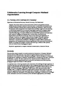
(a)

(b) Figure 3.1: Traces of one host’s behavior allow me to assess my architecture’s potential for true positives without the experimental overhead of an actual network of peers. By sampling the behavior of some binary on one host at different moments in time, as in (a), I can simulate sampling the behavior of that binary on multiple hosts at one moment in time, as in (b), as though the binary began executing on those hosts at different times (i.e., at different T0 ). prototype system, in order to focus on my proposed IDS’s risk of false positives in the actual wild. I select Windows XP with Service Pack 2 (SP2) for my simulation of peers, as the platform offers a richness of available worms (important in any behavioral study) and is a perpetual recipient of innovative attacks. And I utilize that platform’s native API, the nearest equivalent of Linux’s and UNIX’s system calls, as my proxy for behavior. For some time, patterns of system calls have proven to be effective summaries of processes’ behavior on Linux and UNIX [21, 30, 61, 78, 79]. With Windows’s native API officially undocumented, not to mention closed-source, monitoring thereof does prove a challenge itself (Sections 3.2.1 and 4.2.1). Using traces of calls into kernel


36

space by 9 worms and 25 non-worms, I ultimately apply my two measures of similarity to quantify the likelihood that snapshots of calls into kernel space do, in fact, belong to the same executable. To be sure, mere traces of processes might not perfectly reflect “normal activity,” if such can even be said to exist. But, insofar as I gather my traces in environments as deterministic as possible, I argue that they actually allow me to estimate lower bounds on peers’ ability to detect or mistake worms; it’s hard to imagine programs more cyclical (and thus worm-like) than those executing repeated tests or taking no input. In the section that follows, I pose a trio of questions that collectively motivate my simulations. In Section 3.2, I present the methodology with which I approached those questions. In Section 3.3, I present my results.

3.1

Questions

To detect novel worms by leveraging collaborative analysis of peers’ runtime behavior, I must demonstrate that worms tend to stand out in traces of system behavior based on calls to system services. Given two or more samples from those very same traces (i.e., snapshots of behavior), distinguishing an attacking worm from an otherwise benevolent application reduces to the following three questions. (1) How likely is a worm to look like itself ? The more similar a worm’s execution during some window of time to its execution during any other, the more capable should peers be to correlate actions. Moreover, the more similar a worm


37

with respect to itself, the less it should matter when peers sample their behavior. I thus inquire as to whether worms are temporally consistent. The more temporally consistent, the higher my architecture’s chances of true positives. (2) How likely is a non-worm to look like itself ? The more similar a non-worm’s execution during some window of time to its execution during any other, the more likely might peers be to think it a worm. I thus inquire as to whether nonworms are temporally consistent. The more temporally consistent, the higher my architecture’s chances of false positives. (3) How likely is a non-worm to look like a worm? The more similar a non-worm’s execution to that of a worm, the more likely might peers be to mistake the benign for the malevolent, I thus inquire as to whether worms manifest similarities with non-worms. The more similar actual worms are to actual non-worms, the more likely my architecture is to overstate an outbreak’s severity by mistaking the latter for former.

3.2

Methodology

Windows XP SP2’s native API comprises 284 functions, known also as system services, implemented in kernel space by NTOSKRL.EXE and exposed with stubs in user space by NTDLL.DLL, against which most higher-level Win32 APIs are linked. When called to invoke a system service, a stub in NTDLL.DLL invokes SharedUserData!SystemCallStub after moving into register EAX the service’s service ID and into register EDX a pointer to the call’s arguments. To trap from user- to kernel-


38

mode, SharedUserData!SystemCallStub then executes Intel’s SYSENTER instruction (for the Pentium II and newer) or AMD’s SYSCALL instruction (for the K7 or newer).1 Control is ultimately passed to _KiSystemService, which dispatches control to the appropriate service by indexing into _KeServiceDescriptorTable for the service’s address and number of parameters using the value in EAX. By inserting trampolines into this table can I effectively trace all processes’ behavior [17, 24, 25, 28, 58, 66].

3.2.1

Wormboy 1.0

To capture the behavior of Windows XP SP2 with respect to its system services, I implemented Wormboy 1.0, a kernel-mode driver that inserts hooks into _KeServiceDescriptorTable before and after all but two system services. (By default, _KeServiceDescriptorTable is read-only, so Wormboy first disables the WP bit in register CR0 [64, 77]. Alternatively, protection of kernel memory itself could be relaxed, albeit dangerously, by creating registry key HKEY LOCAL MACHINE\ SYSTEM\CurrentControlSet\Control\Session Manager\Memory Management\ EnforceWriteProtection with a DWORD value of 0x0 [68].) However, Windows XP SP2 appears to make certain assumptions about system services NtContinue and NtRaiseException, whereby it attempts to manipulate the stack frame based on register EBP [67]. Inasmuch as my hooks insert a frame of their own, I do not hook those particular services in order to avoid system crashes. Inspired by Strace for NT [68], as well as by work by Nebbett [54] and Dabak et al. [17], Wormboy 1.0 not only captures a call’s service ID and input parameters, 1

On older CPUs, SharedUserData!SystemCallStub executes a slower INT 2e instruction.


39

but also its output parameters and return value, along with a caller’s name, process ID, thread ID, and mode. Though Wormboy could ultimately serve as the core of a real-time defense, this particular version captures all such data to disk, timestamping and sequencing each entry per trace, thereby allowing me to experiment offline with different approaches to detection.

3.2.2

Traces of Worms and Non-Worms

To validate my claim of collaborative detection’s efficacy, I look to some of Windows XP SP2’s fastest worms and most common non-worms to date. I ultimately base my results on traces of 9 variants of worms and 25 non-worms, including 10 commercial applications and 15 binaries native to Windows XP SP2. Table 3.1 lists each of my subjects; I call the worms by their names according to AVG Free Edition 7.0.322 [23]. For each worm, I traced its live activity for 15 minutes, more than enough for its recurrent behavior to surface. For each commercial application save one, I traced its execution under PC Magazine’s WebBench 5.0 [56] or PC World’s WorldBench 5 [57] benchmarking suites. Separately, I traced Nullsoft Winamp 5.094 as it played an MP3 of James Horner’s 19-minute “Titanic Suite,” encoded at 160 kbps. For each native binary, I traced its execution during 24 hours of user-free intervention. I now base my results on all of these traces.


Worms

40

Non-Worms Commercial Applications

Windows XP SP2 Binaries

I-Worm/Bagle.Q

Adobe Photoshop 7.0.1

alg.exe

I-Worm/Bagle.S

Microsoft Access XP SP2

csrss.exe

I-Worm/Jobaka.A

Microsoft Excel XP SP2

defrag.exe

I-Worm/Mydoom.D

Microsoft Outlook XP SP2

dfrgntfs.exe

I-Worm/Mydoom.F

Microsoft Powerpoint XP SP2

explorer.exe

I-Worm/Sasser.B

Microsoft Word XP SP2

helpsvc.exe

I-Worm/Sasser.D

Network Benchmark Client 1.0.3

lsass.exe

Worm/Lovesan.A

Nullsoft Winamp 5.094

msmsgs.exe

Worm/Lovesan.H

Windows Media Encoder 9.0

services.exe

WinZip 8.1

spoolsv.exe svchost.exe wmiprvse.exe winlogon.exe wscntfy.exe wuauclt.exe

Table 3.1: Worms and non-worms whose traces I analyzed with Wormboy 1.0.

3.3

Results

I now answer my own Section 3.1 by way of experimental results. I first assess worms’ degrees of temporal consistency. I then assess non-worms’ degrees of the same. Finally, I consider just how similar actual worms might be to actual non-worms.

3.3.1

How likely is a worm to look like itself ?

A worm is remarkably likely to look like itself, though it depends on the measure of similarity. I find that, while Levenshtein distance allows us to notice with near certainty (at least 95%) the similarity, with respect to themselves, of I-Worm/Sasser.D,


I-Worm/Bagle.Q I-Worm/Bagle.S I-Worm/Jobaka.A I-Worm/Mydoom.D I-Worm/Mydoom.F I-Worm/Sasser.B I-Worm/Sasser.D Worm/Lovesan.A Worm/Lovesan.H

41 5 14% 14% 59% 92% 17% 60% 95% 99% 47%

15 11% 11% 50% 81% 31% 54% 97% 98% 95%

30 10% 11% 69% 73% 41% 72% 93% 93% 93%

60 5% 6% 76% 87% 60% 87% 87% 87% 87%

Table 3.2: Probability with which two peers, upon exchanging snapshots of their internal behavior, can decide using Levenshtein distance alone that they are, more likely than not, both executing the same worm during some window of time, for window sizes of 5, 15, 30, and 60 seconds. In other words, percentages of all possible pairs of samples from some worm for which 1 − max(|Sd1 |,|S2 |) > 0.5, where S1 and S2 are snapshots, treated as ordered sets, and d is the Levenshtein distance between them. I call these percentages degrees, τ , of temporal consistency.

Worm/Lovesan.A, and Worm/Lovesan.H, using a window size of 15 seconds, the metric proves less effective on other variants (Table 3.2), even for windows as wide as 30 or 60 seconds. Bagle’s variants, in particular, appear resistant to classification as temporally consistent using the metric, with no more than 14% of possible pairs of snapshots resembling each other. The disparity, though significant, is not surprising, if we consider the traces themselves. For instance, whereas Worm/Lovesan.A (Figure 3.2) and I-Worm/Sasser.B (Figure 3.3) manifest obvious, nearly constant, patterns, I-Worm/Bagle.Q (Figure 3.4) boasts a less obvious pattern, clouded by overlapping frequencies. With less precise measures, though, I can filter such noise. If I consider only calls’ intersection but not relative frequencies, more more trends are apparent. I now


42

3000

2500

number of calls

2000

1500

1000

500

0 0 84 0 81 0 78 0 75 0 72 0 69 0 66 0 63 0 60 0 57 0 54 0 51 0 48 0 45 0 42 0 39 0 36 0 33 0 30 0 27 0 24 0 21 0 18 0 15 0

12 90

60 30

0

time (seconds) NtAllocateVirtualMemory

NtClose

NtCreateFile

NtDeviceIoControlFile

NtRemoveIoCompletion

NtWaitForSingleObject

NtDelayExecution

Figure 3.2: Calls to system services by Worm/Lovesan.A per 30-second window of time. Point (i, j) indicates j calls to some service between times i and i + 30. Both Levenshtein distance and intersection capture this worm’s pattern of activity. notice with near certainty (97%), using a window size of 15 seconds, every one of our worms save Bagle; but now even Bagle appears temporally consistent with high τ (Table 3.3). Still worthy of note, though not unexpected, is Worm/Lovesan.H, which resists detection, no matter my metric, using a window size of 5 seconds. Such narrow windows simply fail to capture this worm’s periodicity (Figure 3.5); wider windows do capture its periodicity (Figure 3.6).


43

500 450 400 number of calls

350 300 250 200 150 100 50

90 12 0 15 0 18 0 21 0 24 0 27 0 30 0 33 0 36 0 39 0 42 0 45 0 48 0 51 0 54 0 57 0 60 0 63 0 66 0 69 0 72 0 75 0 78 0 81 0 84 0 87 0

60

30

0

time (seconds) NtClose

NtConnectPort

NtCreateFile


NtReadFile

NtWriteFile

Figure 3.3: Calls to system services by I-Worm/Sasser.B per 30-second window of time, representative of worms’ tendency toward simplicity and periodicity. Point (i, j) indicates j invocations of some system call between times i and i + 30. Omitted for visual clarity are similar patterns of invocations of other system calls. As with Worm/Lovesan.A (Figure 3.2), windows of 30 seconds are sufficient to capture this worm’s cycles. It is on this worm’s snapshots that Chapter 2’s Figures 2.3 and 2.4 were based.

3.3.2

How likely is a non-worm to look like itself ?

A non-worm is not nearly as likely to resemble itself as is a worm to resemble itself. Of all the non-worms examined, only Nullsoft Winamp and alg.exe boasted traces for which more than 90% of 15-second snapshots resembled each other, no matter the metric (Figure 3.7). And only alg.exe boasted a trace for which more than 90% of 30-second snapshots resembled each other, no matter the metric. But alg.exe, during my 24-hour run, made only 2,295 calls to system services, an average of no more than one per second. By contrast, even the “slowest” of worms, I-Worm/Jobaka.A, averaged 64 such calls per second. Insofar as processes averaging


44

2500

number of calls

2000

1500

1000

500

0 0 84 0 81 0 78 0 75 0 72 0 69 0 66 0 63 0 60 0 57 0 54 0 51 0 48 0 45 0 42 0 39 0 36 0 33 0 30 0 27 0 24 0 21 0 18 0 15 0

12 90

60 30

0


NtDelayExecution


NtQueryDirectoryFile

NtQueryInformationFile

NtSetInformationFile

NtUnmapViewOfSection


Figure 3.4: Calls to system services by I-Worm/Bagle.Q per 30-second window of time. Point (i, j) indicates j calls to some service between times i and i+30. For visual clarity, less frequently called system services are not pictured. Levenshtein distance fails to capture this worm’s pattern of activity because of overlapping frequencies; intersection does capture the pattern. nearly zero calls per second do not likely belong to fast-moving worms, I can simply require that snapshots not be so empty for some process to be deemed a worm. Nullsoft Winamp, by contrast, averaged 896 calls to system services per second, so its high degree of temporal consistency necessitates more intelligent filtration. I explore filters for cases like it in the next chapter.


I-Worm/Bagle.Q I-Worm/Bagle.S I-Worm/Jobaka.A I-Worm/Mydoom.D I-Worm/Mydoom.F I-Worm/Sasser.B I-Worm/Sasser.D Worm/Lovesan.A Worm/Lovesan.H

45 5 80% 82% 99% 99% 99% 99% 99% 99% 49%

15 76% 76% 97% 97% 97% 97% 97% 97% 97%

30 81% 73% 93% 93% 93% 93% 93% 93% 93%

60 76% 78% 87% 87% 87% 87% 87% 87% 87%

Table 3.3: Probability with which two peers, upon exchanging snapshots of their internal behavior, can decide using intersection alone that they are, more likely than not, both executing the same worm during some window of time, for window sizes of 5, 15, 30, and 60 seconds. In other words, percentages of all possible pairs of samples |S1 ∩S2 | from some worm for which max(|S > 0.5, where S1 and S2 are snapshots, treated 1 |,|S2 |) as unordered sets. I call these percentages degrees, τ , of temporal consistency.

3.3.3

How likely is a non-worm to look like a worm?

Through exhaustive comparison of every possible snapshot from each worm against every possible snapshot from each non-worm, I find that only one non-worm’s behavior resembles, more often than not, that of a worm: Network Benchmark Client is similar to I-Worm/Jobaka.A, I-Worm/Sasser.B, and I-Worm/Sasser.D, if intersection is the metric. But the resemblance is neither surprising nor troubling, as Network Benchmark Client is practically a worm itself, designed to fork 5 threads, each of which induces stress on a server by initiating TCP sockets in rapid succession.


46

number of calls

500 400 300 200 100 0 0

895


NtCreateFile



Figure 3.5: Calls to system services by Worm/Lovesan.H per 5-second window of time. Point (i, j) indicates j calls to some service between times i and i+5. For visual clarity, less frequently called system services are not pictured; similarly are most xaxis labels omitted. 5-second windows are not adequate to capture periodicity in this worm’s behavior.

3.4

Summary

Host-based detection of worms via collaboration among peers is possible. I base this claim on simulations that have allowed me to analyze 9 variants of worms and 25 non-worms on Windows XP SP2. These results follow from a definition of anomalous behavior as correlation among otherwise independent peers’ behavior. For the set of worms and non-worms tested, I find that two peers, upon exchanging one window’s worth of snapshots of their internal behavior, defined in terms of frequency distributions of calls to system services, can detect execution of some worm between 76% and 97% of the time because of worms’ temporal consistency. More significantly, the risk of false positives appears low. In the chapter that follows, I corroborate these results and propose filters for worm-like non-worms. I transition from simulation to actual implementation and deployment of a prototype of my vision. I focus, in particular, on my system’s likelihood


47

number of calls

1200 1000 800 600 400 200

,

0 0

895


NtCreateFile



Figure 3.6: Calls to system services by Worm/Lovesan.H per 15-second window of time. Point (i, j) indicates j calls to some service between times i and i + 15. For visual clarity, less frequently called system services are not pictured; similarly are most x-axis labels omitted. 15-second windows are adequate to capture periodicity in this worm’s behavior. of false positives in the wild. I continue to exploit temporal consistency, but I adopt for the next chapter the superior of this chapter’s measures—that based on intersection—as it has herein proved tolerant not only of offsets in timing but also of differences in hosts’ speeds and configuations. Hereinafter, then, I shall judge the similarity of two snapshots, S1 and S2 , by way of S1 ∩ S2 .

48

2

2

2

2

2

2

2

2

2

2

2

2

2

2

.$

$$ / / 2, '+/ $ * ,$ & $ . $ $$ $ $ & $ $, -. $ $& $ 5 .* & - $ 5 ,& + -' $ 5 $. ' 5 '+/ 4 4. +

2

"

" -' " 8,"

% $$ & $ ! -. " & ' )* $ $ ' -. /+" + $ ( * -. -. $ .. , " $ / $ + $ " $ /+ /+"3 12. "0) ") 6 - 5 4+ " 0 " ) ) +5 . $ , "0 " ) /+ -' )" " " +" -' 64 0) ) $ ' 5 /+ .* "0 " ) $" " )" -' "7 ) "1 , - ' '. " + %

$$

! " #

τ


Figure 3.7: Degrees, τ , of temporal consistency of worms versus non-worms, using 15-second windows. Of all the non-worms examined, only Nullsoft Winamp and alg.exe boasted traces for which more than 90% of 15-second snapshots resembled each other, no matter my metric for similarity. All but two of the worms examined, meanwhile, boasted τ > 90%.

Chapter 4 False Positives In this chapter, I build upon the results of the previous chapter and evaluate my ideas “in the wild.” I implement and deploy an actual prototype of my vision, Wormboy 2.0, to a network of 29 hosts running Windows XP SP2. I use this implementation to monitor and analyze 10,776 processes, inclusive of 511 unique non-worms (873 if one considers unique versions to be unique non-worms). I further investigate a hostbased, collaborative architecture’s rates of true positives and false positives, focusing all the more on the latter. As a result of this prototype, I identify properties that distinguish worms from nonworms. Using those properties, my architecture accurately classifies 99% of processes as non-worms. I also find that this collaborative architecture, using patterns of system calls and simple heuristics, can detect worms running on multiple peers. And, because of the unlikely appearance on many peers simultaneously of non-worm processes with worm-like properties, I find that collaboration among peers significantly reduces the risk of false positives. In the section that follows, I offer a new trio of questions. In Section 4.2, I describe Wormboy’s new role and offer implementation details. In Section 4.3, I validate my 49

Chapter 4: False Positives

50

vision’s efficacy on real systems: I quantify the number of non-worm processes that might, if not handled carefully, be mistaken for worms by a collaborative architecture; I establish empirically that a collaborative network can detect processes with similar behavior running on multiple hosts; and I demonstrate that collaboration among peers reduces the risk of false positives.

4.1

Questions

To validate the efficacy of host-based, collaborative detection in the wild with real systems, I now focus on this trio of questions. (1) Are non-worms, like worms, temporally consistent? If so, I must identify properties that distinguish the two. Alternatively, I must identify thresholds beyond which τ actually indicates worms. (2) Can I detect processes with similar behavior on multiple hosts? If so, I can detect the outbreak of a worm, the behavior of which across hosts is likely to be similar. Again, bounded by time as are fast-moving worms by definition, there are only so many ways for them to achieve some effect on a host quickly. A worm’s filename and executable, by contrast, can be too easily altered during propagation (as through metamorphosis) and are, thus, less reliable than more dynamic techniques. Presumably, the more “worm-like” a process (i.e., the more temporally consistent), the more likely I am to detect it if running on multiple hosts.


51

(3) Can I avoid mistaking popular non-worms for worms? I cannot assume that processes common to many hosts (e.g., explorer.exe) are necessarily worms, lest I infer incorrectly that an attack is in progress. And I should not confuse a non-worm running on one host with a worm running on another, even if behaving similarly, lest I overstate an outbreak’s severity. To answer these questions, I transition from simulation to actual implementation of my prototype. I deploy Wormboy 2.0 to dozens of hosts running hundreds of non-worms in order to evaluate collaborative detection’s efficacy in the wild through collection and analysis of real-world data. In the section that follows, I offer implementation details for Wormboy 2.0 to make clear my data’s origins and manner of collection.

4.2

Methodology

Again modeling hosts’ behavior in terms of snapshots, I implemented Wormboy 2.0, a prototype of a host-based, collaborative system with one purpose: to collect and analyze snapshots from real systems. Ultimately the foundation for a worm-focused IDS, Wormboy now includes both client and server sides that, together, implement a network of peers per my vision (Figure 2.1). With one such network alone, I am able to collect and analyze data from real-world hosts.


4.2.1

52

Wormboy 2.0: Peers’ Client

On the client side, Wormboy 2.0 is implemented as a cooperation between a kernel-mode driver (WORMBOY.SYS) and a user-mode application (WORMBOY.EXE), both written in C. Inspired by work by Sabin [68], Nebbett [54], Harris [26], and Dabak et al. [17], Wormboy’s client currently supports Windows XP with Service Pack 2. With minor modifications, Wormboy’s client could also support Windows NT (with and without Service Packs 3 through 6), Windows 2000 (with and without Service Packs 1 through 4), Windows XP (with and without Service Packs 1 and 2), and Windows 2003 Server (with and without Service Pack 1). Upon load, WORMBOY.SYS hooks all but three system services by inserting trampolines into _KeServiceDescriptorTable. (For this version of Wormboy, I no longer hook NtQueryInformationProcess, as my other hooks invoke undocumented features of this service themselves.) These hooks effectively log (to unpaged memory) each invocation of a system service during some window of time, capturing not only the call’s service ID but also the caller’s PID and path. At the end of each window, WORMBOY.EXE polls WORMBOY.SYS for that window’s snapshots, the structure of which appears in Figure 4.1. The application then transmits those snapshots to Wormboy’s snapshot server via XML-RPC [27, 93]. I propose more efficient alternatives to XML-RPC for snapshots’ transport in Section 5.3. For reasons of privacy, Wormboy 2.0 does not capture hooked calls’ parameters. The implication, a result of Windows XP SP2’s design, is that it cannot detect network activity with certainty using service IDs alone. For my answers to Section 4.1’s questions, I therefore infer network activity from frequent calls to NtCreateFile (the


53

typedef struct { ULONG counts[NUM_SERVICES]; ULONG pid; CHAR path[MAX_PATH]; } snapshot; Figure 4.1: Wormboy 2.0’s definition of a snapshot. On the client-side, Wormboy’s kernel-mode driver maintains in non-paged memory one of these structures for each live process. On some schedule, Wormboy’s user-mode application polls the driver for those structures (after which the driver zeroes counts) and marshals them over XML-RPC to Wormboy’s snapshot server for analysis. service involved in sockets’ creation), NtDeviceIoControlFile (the service involved in packets’ transmission), and NtCloseFile (the service involved in sockets’ termination) [33]. Though I might overestimate some processes’ network activity as a result, that risk actually motivates my exploration of additional heuristics for worms’ detection (Section 4.3.1).

4.2.2

Wormboy 2.0: The Snapshot Server

On the server side, Wormboy 2.0’s snapshot server is implemented quite simply in Java as a XML-RPC listener (WormboyD). Upon receipt of a window’s worth of snapshots from Wormboy clients, WormboyD analyzes the structures for similarities, as per my measure based on intersection. The server then logs the results of its analyses to disk for later review. For scalability’s sake, I explore efficient implementations (in C++) of snapshots’ comparison in Section 5.4.


4.3

54

Results

I present in this section my results for Section 4.1’s inquiries. To answer those questions using real-world data, I deployed Wormboy 2.0 for 24 hours to a network of 29 actively used, independent hosts (spread across domains throughout North America) running Windows XP SP2. With this deployment, I was ultimately able to monitor and analyze 10,776 processes, inclusive of 511 unique non-worms (873 if we consider unique versions to be unique non-worms). Though these hosts, as real systems on the Internet, were by nature exposed to worms, I did not inject worms into this network myself. Nor did I set out to detect actual worms; this chapter’s focus remains on non-worms and the avoidance of false positives. I present this experiment’s results in turn. I first quantify the number of nonworm processes that a collaborative network might tend to mistake for worms, were it not for certain properties unique to the latter (Section 4.3.1). I then demonstrate empirically, using non-worms with worm-like properties as proxies for worms, that a collaborative network can, in fact, detect worms executing on multiple hosts (Section 4.3.2). Finally, I show how collaboration among peers reduces the likelihood of false positives (Section 4.3.3).

4.3.1

Identifying

τ , r, and r0

In Chapter 3, I investigated the degree to which 25 non-worms were temporally consistent. Through simulation, I found that only 2 of those 25 (8%) boasted traces for which τ > 90% using windows of 15 seconds; only one of the 25 boasted a trace for


55

which τ > 90% using windows of 30 seconds. With simple heuristics, I then distinguished those non-worms from worms, despite their apparent similarity. For instance, I considered for each process not only its τ but also its rate of calls, r, into kernel space. In particular, one potential false positive averaged no more than r = 1 call into kernel space per second, whereas even the “slowest” of worms, I-Worm/Jobaka.A, averaged r = 64 calls per second. Insofar as processes averaging nearly zero calls per second do not likely belong to fast-moving worms, I required that large τ , to be worrisome, be accompanied by non-negligible rates of calls (e.g., r ≥ 64). By way of analysis with Wormboy 2.0 of not 25 but thousands of processes, I have since found it advantageous to identify an additional property besides τ and r that distinguishes worms from non-worms. For each of the processes for which WormboyD received snapshots over the course of 24 hours, I reviewed up to an hour’s worth of data, exhaustively measuring the similarity of each snapshot received during that frame against every other snapshot received during the same. No matter my windows’ size, I find that at least 315 of the 10,776 non-worm processes boast τ ≥ 76% and r ≥ 64. Those 315 processes belong to 85 (17%) of our 511 unique non-worms. But if I further require that some process actually utilize the network at a rate, r0 , no slower than that of our slowest of worms, I fare even better. I now find, using a window of 15 seconds, that only 145/10, 776 ≈ 1% of processes appear to be worms and, equivalently, that 99% of processes appear not to be worms. And those 145 processes belong to just 15 (2.9%) of our 511 unique non-worms (Table 4.1). I summarize these results in Table 4.2. Figure 4.2, meanwhile, testifies that worms do tend to stand out among non-worms based on their values of τ , r, and r0 , plotting in three


56 15

aexplore.exe aolsoftware.exe ApntEx.exe BESClient.exe CCPROXY.EXE cvpnd.exe explorer.exe iexplore.exe ntbackup.exe OUTLOOK.EXE QCWIZARD.EXE SNDSrvc.exe sshd.exe ViewMgr.exe war3.exe

30 1.EXE aexplore.exe aolsoftware.exe ApntEx.exe BESClient.exe ccApp.exe CCPROXY.EXE cvpnd.exe explorer.exe iexplore.exe ntbackup.exe OUTLOOK.EXE QCWIZARD.EXE sshd.exe ViewMgr.exe war3.exe wmplayer.exe WRSSSDK.exe

Table 4.1: Nineteen non-worms that exhibit worm-like behavior, for windows of 15 and 30 seconds. Of the 511 unique non-worms in my study, I might mistakenly classify as worms just 15 (2.9%) using windows of 15 seconds and 18 (3.5%) using windows of 30 seconds. Processes common to both windows are aligned for visual clarity.

dimensions each of those values for worms and non-worms alike. Worthy of note is that the worms cluster together. The figure also makes clear how a worm might try to “hide” among non-worms: by lowering its rate of network activity. That particular recourse, though, would only slow a worm down, which, again, would constitute success for my IDS’s collaborative approach. Though I earlier found through simulation 8% (2 of 25) non-worms to resemble worms, I now lower that bound to 1%, using real-world data filtered not only by τ and r but also by r0 . Other filters may very well be possible. But that only 15 of


Non-Worm Processes . . . w/ τ ≥ 76%, r ≥ 64 . . . w/ τ ≥ 76%, r ≥ 64, r 0 > δ

57 15 s 10,776 (511) 351 (77) 145 (15)

30 s 10,776 (511) 315 (85) 112 (18)

Table 4.2: Results of exhaustive, worst-case examination of 10,776 non-worm processes for worm-like behavior, where τ denotes a process’s degree of temporal consistency, r denotes a process’s rate of calls to system services, r0 denotes a process’s rate of network activity, and δ denotes a threshold (the slowest rate of network activity witnessed among my 9 worms). Listed parenthetically are the numbers of unique non-worms (irrespective of version) to which processes belong. With intelligent filtration, as few as 15 (2.9%) of 511 unique non-worms resemble worms.

511 remain after these filters alone reinforces the potential of collaborative detection, insofar as so few out of hundreds of non-worms might potentially evince worm-like behavior on many hosts at once.

4.3.2

Detecting Processes across Peers

Chapter 3 suggests that worms can be detected across peers because of worms’ degrees of temporal consistency (e.g., τ > 90%), while the current chapter maintains that certain “worm-like” non-worms, if not properly filtered, might be detected as well. I now confirm these hypotheses in this section. In particular, I look for positive correlation between some process’s τ and the probability with which our collaborative network recognizes that process’s execution on multiple peers. Rather than inject worms into my network of 29 hosts, I look to the network’s most worm-like of nonworms (Section 4.3.1) as proxies for worms. For the purposes of this inquiry, I treat those non-worms with particularly high τ as representative of worms. I expect that large τ should imply high rates of recognition, whereas the smallest of τ should imply


58

Figure 4.2: τ versus r versus r0 for worms and non-worms, averaged over an hour’s worth (or less) of execution for each process, presented in three dimensions to highlight worms’ clustering. Axes are scaled for visual separation of worms from non-worms. few, if any, matches in snapshots from peers. If I examine each of my 29 peers’ non-worms over 24 hours, I find that only for large τ are multiple peers likely to recognize a common process. Figure 4.3 depicts this result, plotting non-worms’ rates of recognition against non-worms’ degrees of temporal consistency. I define rate of recognition as follows: if some non-worm is executing during some window on n ≥ 2 peers, and we determine that m such instances are similar, then that non-worm’s rate of recognition for that window is said to be m/n. By similar, I mean that, for each pair of processes among the m,


59

Figure 4.3: Rates of recognition of non-worms as a function of those non-worms’ degrees, τ , of temporal consistency, averaged over an hour’s worth (or less, for shortlived processes) of activity during 24 hours of analysis using windows of 30 seconds. If some non-worm is executing during some window on n peers, and m such instances are judged similar, then that non-worm’s rate of recognition is said to be m/n. All non-worms depicted boasted rates of calls into kernel space, r, greater than 64 per second (the rate of my slowest of worms). As I expected for actual worms, only processes with large τ are detected at non-negligible rates. Dots representing large τ but low rates of detection belong to processes that, because of their brevity or relative unpopularity, tended not to appear among my 29 hosts simultaneously. Shaded is this figure’s upper-right quadrant, which includes six non-worms with τ ≥ 76% that were detected at least 10% of the time. I expect actual worms to fall within this quadrant as well, per Chapter 3. |S1 ∩S2 | max(|S1 |,|S2 |)

> 0.5, where S1 and S2 are snapshots, for at least 76% (Chapter 3’s least

worrisome τ ) of the snapshots submitted for the processes (over the course of an hour). Informally, I judge two processes similar if at least 76% of their snapshots look “mostly the same.” This judgement is thus independent of those processes’ filenames and any other distinguishing marks (e.g., hashes) that might be all too easily altered by worms’ authors. In terms of cliques, a rate of recognition of m/n for some process during some


60

window implies recognition of an m-clique of similarity among snapshots from all of our peers, n of which are actually executing that process. (It is not necessarily the case that an n-clique also exists during that window, as processes with τ < 100% might not “look the same” across all peers during some window.) Because no cliques in my study exceeded m = 6, I compiled the results for Figures 4.3 and 4.4 using brute-force analysis. Cooperative networks boasting larger n (and, in turn, larger m) demand more efficient approaches, per Chapter 5. To be clear, n is not necessarily the network’s size but, rather, the number of hosts on the network executing some non-worm. As such, m/n is simply a rate of recognition, not a rate of infection. Though peers’ average rates of recognition are not strictly correlated with rising τ , in no 30-second window during my 24 hours of data do multiple peers detect processes common to them at non-negligible rates if those processes’ τ are below 65%. For τ ≥ 65%, I do detect common processes at non-negligible (i.e., double-digit) rates, except for processes (whose points fall on Figure 4.3’s x-axis) that, because of their brevity or relative unpopularity, tended not to appear among my 29 hosts simultaneously. My intent, though, is to detect fast-moving worms, whose activity, by nature, is more likely to be ongoing than brief. That processes with τ ≥ 65% are, in fact, recognized across peers reinforces host-based, collaborative detection’s potential, inasmuch as τ for every one of my worms was at least 76% (Chapter 3). Because of worms’ relatively high degrees of temporal consistency, I expect they will fall within Figure 4.3’s shaded, upper-right quadrant, as do 6 of my study’s most worm-like non-worms.


61

rates of recognition (%)

100 ave

max

75 50 25

Ap nt Ex gc .e as xe S ib er mm v. es ex sa e ge s. ex Ap e oi nt .e wi xe na mp .e xe av gw tr .e il xe li * an ex .e pl xe or er .e xe vs mo n. fi ex re e fo go x. og e le xe ta lk . po ex in e t3 2 ss .e my xe pi cs .s Rt cr vs ca n. vi ex ew e mg r. ns e cs xe rv ce zl .e cl xe ie nt .e it xe un es .e xe sk yp e. se ex rv e ic es * .e OU xe TL OO K. sv EX ch E os t. ex e

*

0

non-worm

Figure 4.4: Average and maximal rates of recognition for non-worms whose average rates of recognition exceed 1%. Figure 4.3 plots these same average rates against non-worms’ degrees of temporal consistency. Only three of these non-worms (*) are worrisome in that they also appear in Table 4.1, boasting worm-like τ , r, and r0 .

4.3.3

Avoiding False Positives

Because my intent is to detect worms rapidly (ideally within, say, a single, 30second window), it is necessary to examine not only non-worms’ average rates of recognition but also their worst-case, maximal rate of recognition (i.e., the maximum of m/n seen over time). After all, even if some non-worm goes undetected most of the time, a single window’s worth of similar behavior across many peers might induce a false positive, whereby some non-worm is judged a worm. Figure 4.4 contrasts average and maximal rates of recognition for those non-worms whose average rates of recognition exceed 1%. Particularly worrisome are those non-worms whose maximal rates of recognition are 50% < m/n ≤ 100%, the result of which is that, on occasion, those non-worms were detected on most, if not all, of the hosts on which they were running. But in none of those cases were the non-worms running on most of the peers in my network. In fact, in none of these cases was m (or n) greater than 4, whereas my network consisted


62

of 29 peers, an apparent “infection” rate, ι, of 4/29 ≈ 14%. Accordingly, provided I set my threshold for detection at 14% (i.e., require, for a worm to be assumed present, that some process appear similar on ι > 14% of peers), my cooperative of 29 peers avoids a false positive. In other words, a high rate of recognition (m/n) does not imply a high rate of infection or, rather, in the case of non-worms, a likelihood of false positives. Based on these results, I propose, for now, ι = 14% as a threshold for host-based, collaborative detection: if a worm-like process (i.e., with worrisome r and r0 ) appears on more than 14% of peers in a network, a worm shall be assumed present. With additional data could this threshold be fine-tuned. My collaborative network’s potential for false positives is indeed less than Figure 4.4 suggests. If I cross-reference those non-worms in Figure 4.4 with those in Table 4.1, I find that only three are “worm-like,” insofar as they appear in both: ApntEx.exe, explorer.exe, and OUTLOOK.EXE. Filtration by τ , r, and r0 therefore limits our risk of false positives to the actions of just three of 511 non-worms. At least two of these non-worms (iexplore.exe and OUTLOOK.EXE) do involve frequent network activity, but not so frequent as my fastest of worms (Chapter 3). Moreover, it may, in fact, prove feasible to whitelist these most popular of non-worms (as with read-only hashes of their executables). My focus in this thesis remains on more generalized techniques. Of course, not only might false positives induce an IDS to infer incorrectly that an attack is in progress, they might also induce an IDS to overstate an actual outbreak’s severity. By confusing non-worms with actual worms, an IDS might conclude that


63

more hosts are infected than actually are, the result of which might be a premature or unnecessarily severe reaction, depending on the IDS’s mechanism for response. To determine the likelihood with which non-worms might resemble actual worms, I performed an exhaustive comparison of snapshots from my 19 most worm-like non-worms (15 of which appeared worm-like using windows of 15 seconds and 18 of which appeared worm-like using windows of 30 seconds) among my 511 unique non-worms (Table 4.1) with snapshots from Chapter 3’s 9 worms. The results are striking: 14 of the 19 non-worms appear similar to actual worms. More formally, the percentage of all possible pairs of snapshots for which

|S1 ∩S2 | max(|S1 |,|S2 |)

> 0.5 itself exceeds

50% for these 14 non-worms and is even as high as 100% for one (Table 4.3). Closer examination of these non-worms’ and worms’ snapshots offers some insight. If I consider, for instance, the most striking of these matches, sshd.exe vis-à-vis I-Worm/Mydoom.F, I see that, while the two manifest remarkable overlap in services utilized, their frequency distributions are markedly different (Figure 4.5), the implication of which is that consideration of either in filtration might, in fact, prove useful in such cases. But it is far simpler to filter based on non-worms’ rates, r0 , of network activity.

4.4

Summary

Inherent in automated, behavior-based IDSes for worms is a risk of false positives. I combat this risk with collaboration among peers. In this chapter, I vetted this idea using my implementation of Wormboy 2.0, a prototype for host-based, collaborative detection. I deployed my prototype to a network of 29 hosts running Windows,


64

where I monitored and analyzed 10,776 processes. Using the data gathered from this network, I exposed the utility of temporal consistency (similarity over time in worms’ and non-worms’ invocations of system calls) in collaborative detection. I identified properties that distinguish non-worms from worms 99% of the time. I found that a collaborative network, using patterns of system calls and simple heuristics, can detect worms running on multiple hosts. And I found that collaboration among peers reduces the risk of false positives because of the unlikely, simultaneous appearance across peers of non-worm processes with worm-like properties.


Non-Worm 1.EXE aolsoftware.exe apntex.exe besclient.exe ccproxy.exe cvpnd.exe

explorer.exe

iexplore.exe OUTLOOK.EXE SNDSrvc.exe sshd.exe ViewMgr.exe wmplayer.exe WRSSSDK.exe

65

Worm(s) I-Worm/Mydoom.F I-Worm/Sasser.D Worm/Lovesan.A I-Worm/Mydoom.F I-Worm/Mydoom.F I-Worm/Sasser.D I-Worm/Jobaka.A I-Worm/Sasser.B I-Worm/Mydoom.F I-Worm/Bagle.S I-Worm/Bagle.Q Worm/Lovesan.H I-Worm/Mydoom.F Worm/Lovesan.A I-Worm/Mydoom.D I-Worm/Mydoom.F Worm/Lovesan.H I-Worm/Sasser.D I-Worm/Mydoom.F I-Worm/Sasser.D I-Worm/Mydoom.F I-Worm/Mydoom.F I-Worm/Mydoom.F

Similarity 58% 74% 56% 97% 77% 73% 66% 64% 85% 61% 60% 58% 85% 71% 54% 64% 97% 72% 100% 74% 67% 51% 89%

Table 4.3: Similarity over time of 14 worm-like non-worms (per Table 4.1) with actual worms, determined using windows of 30 seconds. The striking similarities suggest that further reduction of a collaborative system’s probability of false positives requires further refinements in filtration (e.g., some consideration of calls’ order or relative frequencies).


66

(a) sshd.exe

(b) I-Worm/Mydoom.F Figure 4.5: Snapshots from (a) sshd.exe and (b) I-Worm/Mydoom.F, using windows of 30 seconds. For each window, the frequency of each service’s invocation is depicted as a percentage of the total number of calls into kernel space during that window. For visual clarity, snapshots are unlabeled; distinct shades imply distinct system services. Although sshd.exe and I-Worm/Mydoom.F appear similar to Wormboy (because the two invoke a large, common subset of system calls), the two differ in their relative frequencies of invocations.

Chapter 5 Scalability Thus far, I have focused on my proposed IDS’s potential for true positives and risk of false positives. The question remains, though, of whether this architecture actually scales. I now show in this chapter that collaborative detection indeed scales beyond 29 peers, much like the botnets it intends to detect. And I consider some of the threats thereto. In the section that follows, I provide a framework with which to assess the scalability of my proposed architectures. In Section 5.2, I assess the cost of peers’ monitoring of their own behavior. In Section 5.3, I model the cost of peers’ submission of snapshots. In Section 5.4, I model the most expensive of tasks, actual analysis of snapshots and discovery of cliques.

5.1

Framework for Assessment

As per my architecture (Chapter 2), detection of worms reduces to: (1) self-monitoring by peers of their own behavior; (2) submission of snapshots by peers to a snapshot server; and 67

Chapter 5: Scalability

68

(3) analysis of snapshots for similarities by snapshot server, which itself reduces to: (a) pairwise comparison of snapshots; and (b) searching for cliques across peers, whereby snapshots are vertices and similarities are edges. The scalability of my architecture therefore reduces to the costs of these processes vis-à-vis real-world limits thereupon. In the sections that follow, I model these costs and propose designs for minimization thereof. My proposed units of measure are limited resources: time (i.e., CPU cycles) and space (i.e., bandwidth and memory). To be not only scalable but viable as well, I recognize that my architecture must respect real-world limits on resources. Lest the cure for worms, so to speak, be worse than the disease, my architecture must not prevent peers from getting actual work done. I therefore restrict my own architecture’s design. I assume that it may use megabytes but not gigabytes of peers’ memory (both primary and secondary). I assume that peers can download megabits per second (e.g., 1.5 Mbps) but only upload kilobits per second (e.g., 364 kbps). I assume that snapshot servers have access to less limited resources. And I require that submission of snapshots and analysis thereof be rapid, less than or equal to one window’s worth of time, lest my architecture “fall behind” in its analyses.

5.2

Self-Monitoring By Peers

However peers’ behavior happens to be defined, my architecture assumes some form of constant monitoring thereof. The cost of such monitoring, then, is of par-


Benchmark Adobe Photoshop 7.0.1 Adobe Premiere 6.5 Ahead Software Nero Express 6.0.0.3 Microsoft Office XP SP2 Microsoft Windows Media Encoder 9.0 Mozilla 1.4 MusicMatch Jukebox 7.10 Roxio VideoWave Movie Creator 1.5 WinZip Computing WinZip 8.1

69

Calls 258,549 13,379,755 46,869,089 2,317,059 1,672,449 51,956,045 308,793 2,287,867 4,775,630

Runtime w/o w/ 1574 s 1589 s 1830 s 1864 s 2536 s 2610 s 1054 s 1065 s 2141 s 2164 s 2883 s 3002 s 2680 s 2699 s 1553 s 1569 s 1704 s 1717 s

Overhead 0.95% 1.9% 2.9% 1.0% 1.1% 4.1% 0.71% 1.0% 0.76%

Table 5.1: Results of executing PC World’s WorldBench 5 [57] benchmarking suite without (w/o) and with (w/) Wormboy 2.0’s client running on a 550MHz Pentium III with 384MB RAM atop Windows XP SP2, averaged over 10 runs of the suite, the standard deviations for which varied from 4 to 23 seconds. Wormboy’s average impact on runtime did not exceed 4.1%.

ticular concern, lest my architecture impede peers’ actual work. I evaluate my own proxy for behavior to provide a sense of these costs. With calls into kernel space as this thesis’s proxy, the performance of Wormboy 2.0’s client is of particular concern, lest hooking as many as thousands of calls per second interfere with peers’ actual work. Not only, then, does Wormboy log calls to unpaged memory, it also executes few instructions to perform its logging. To determine Wormboy’s impact on peers, I executed PC World’s WorldBench 5 [57] benchmarking suite without and with Wormboy’s client running on a 550MHz Pentium III with 384MB RAM atop Windows XP SP2. Though further optimization is certainly possible, Wormboy’s impact on peers’ runtime already appears reasonable. Per Table 5.1, Wormboy increased the running time of the suite’s applications by no more than 4.1%.


5.3

70

Submission of Snapshots

The next cost to consider is that of submission of snapshots. As per my architecture, this process involves transmission of some number of bits by some number of peers to some centralized server within some window of time. My architecture assumes neither synchronization of peers’ behavior nor synchronization of snapshots’ submission (Section 2.3). Though peers do submit sets of snapshots every n seconds, they might very well submit at different moments within n-second windows of time. For scalability’s sake, then we can distribute snapshots’ submission over this window of time. Each n seconds, the snapshot server will simply analyze what snapshots it has; the next snapshots received will be analyzed during the next window of time. The bandwidth (in bits per second) required of this centralized server is thus

bandwidth =

number of bits per peer × number of peers . size of window in seconds

(5.1)

Equivalently, the number of peers allowed by a window of some size is

number of peers =

bandwidth × size of window in seconds . number of bits per peer

Per Chapters 3 and 4, windows’ size is best dictated by peers’ own behavior. With system calls my proxy for behavior and intersection my basis for snapshots’ comparison, 30 seconds, for instance, worked well. With bandwidth ultimately limited by dollars or line speeds, at least one parameter remains within in our control: the number of bits per peer also dictates our number of peers.


71

Although Wormboy’s client currently has peers submit snapshots via XML-RPC (for simplicity), more efficient submissions are possible. “Terseness in XML markup is of minimal importance” [98], after all, and XML-RPC is by no means compact. If my architecture is to scale, not only must peers be able to submit snapshots quickly, the receiving snapshot server must be able to handle the load. The fewer bits that peers need to submit, then, the more peers the snapshot server might handle. I look to my data from Wormboy 2.0 (Chapter 4) to motivate more efficient design. Over the course of my 24-hour deployment of Wormboy, my 29 peers submitted a total of 1,029,665 snapshots. In each 30-second window of time, peers submitted between 1 and 185 snapshots each. On average, though, each peer submitted only 22 snapshots, with a standard deviation of 9. However, many of those snapshots prove irrelevant with regard to detection of worms, which, by nature, should involve network activity. On average per window, peers submitted only 3 snapshots involving network activity (i.e., invocation of NtOpenFile, NtDeviceIoControlFile, and NtCloseFile), the implication of which is that peers need not submit the other 22 − 3 = 19. Table 5.2 summarizes these findings. The challenge at hand, then, is to submit an average of 3 snapshots per peer in a format conducive to both transmission and analysis. Of course, snapshots themselves can vary in size. As unordered sets of system services’ IDs, they necessarily range from 1 to 284 in cardinality. Over Wormboy 2.0’s 24-hour deployment, though, I found that, in practice, snapshots contained between 1 and 122 IDs, with small snapshots more common than large (Figure 5.1). The size of a snapshot, on average, was 11 (Table 5.3); the overall median was just 7. If we assume fixed-width encoding of


snapshots per window per peer

snapshots w/ network activity per window per peer

72 median

mean

std. dev.

min.

max.

20

22

9

1

185

3

3

2

0

172

Table 5.2: Numbers of snapshots received per 30-second window from each of my 29 peers over the course of 24 hours, during which my snapshot server received 1,029,665 snapshots in total. On average, each peer submitted 22 snapshots to the snapshot server per window of time. However, on average, only 3 of those snapshots involved network activity (i.e., invocation of NtOpenFile, NtDeviceIoControlFile, and NtCloseFile). The most snapshots ever submitted by a peer for some window was 185 (172 if we only consider those with network activity). As the low standard deviations suggest, that peer proved to be an outlier; it was a research machine running dozens of instances of sshd.exe.

IDs (to avoid computational costs of compression), we need 2 bytes per ID and, thus, 16 × 11 = 176 bits per snapshot on average. In the extreme, though, a snapshot might contain 122 IDs (or, worse, 284), thereby proving 122/11 ≈ 11 (or 284/11 ≈ 26) times larger than usual, the implication of which is 1,100% (or 2,600%) as much work (i.e., comparisons) for the snapshot server receiving that load. For scalability’s sake, I desire more predictable loads. Better, then, to represent snapshots with 36-byte arrays of bits, b0 b1 · · · b283 0000, whereby bi = 1 if and only if ID i belongs in the snapshot. For peers, uploading an average of 3 snapshots per, say, 30-second window, each of which totals just 36×8 = 288 bits, is certainly reasonable. Of greater interest, though, is just how many such snapshots a snapshot server could handle. Assuming overhead of 20 bytes for TCP [60], 20 bytes for IP [59], and 18 bytes for Ethernet [34], each peer’s submission of 3 36-byte snapshots involves upload of 3×36+20+20+18 = 166 bytes (1,328 bits). Accordingly, the bandwidth required by the snapshot server varies


73

160,000

140,000

120,000

frequency

100,000

80,000

60,000

40,000

20,000

0 1

122 sizes of snapshots

Figure 5.1: Sizes of snapshots received (i.e., number of unique system services invoked) per 30-second window from each of my 29 peers over the course of 24 hours, during which my snapshot server received 1,029,665 snapshots in total. Snapshots’ sizes ranged from 1 to 122. On average, peers’ processes each invoked 11 unique system services per window, per Table 5.3. Most snapshots were relatively small in size. Over 140,000 of the 1,029,665 snapshots, for instance, contained the ID of just one system service. linearly with the number of peers, per Equation 5.1. Of the snapshot server, then, 100 peers would demand 1, 328 × 100 number of bits per peer × number of peers = ≈ 4, 427 size of window in seconds 30 bits per second, while as many as 10,000 peers would still only demand approximately 442,667 bits per second, per Table 5.4. Such loads as these are well within reasonable limits (e.g., T-1 speeds). Even if 10,000 peers happen to submit at once, today’s


sizes of snapshots

74 median 7

mean 11

std. dev. 12

min. 1

max. 122

Table 5.3: Sizes of snapshots received (i.e., number of unique system services invoked) per 30-second window from each of my 29 peers over the course of 24 hours, during which my snapshot server received 1,029,665 snapshots in total. Snapshots’ sizes ranged from 1 to 122. On average, peers’ processes each invoked 11 unique system services per window. As the difference between median and mean suggests, most snapshots were relatively small in size, per Figure 5.1.

peers 100 500 1,000 5,000 10,000

bandwidth 4,427 bps 22,133 bps 144,267 bps 221,333 bps 442,667 bps

Table 5.4: Estimates of bandwidth required for transmission of 3 36-byte snapshots from each peer, for various numbers of peers, assuming windows of 30 seconds and overhead of 20 bytes for TCP [60], 20 bytes for IP [59], and 18 bytes for Ethernet [34]. These estimates suggest that my architecture could scale, based on bandwidth alone, to thousands of hosts.

networks (e.g., T-3 speeds) could handle the flow. Of course, resources besides bandwidth are also limited. Servers suffer concurrency limits as well, whereby only so many connections can be handled at once (whether by separate threads or separate processes). But, these days, even 10,000 connections per second are possible [41, 42]. Of course, we cannot spend all of our time simply receiving these snapshots. We must allow time to analyze those snapshots. How many and how fast we might analyze is the next question at hand.


5.4

75

Analysis of Snapshots

Upon receipt of, say, 3 snapshots from each of n peers, analysis thereof must begin. And it must complete before the next window’s worth arrives. The challenge at hand reduces conceptually to searching for cliques in a graph, whereby snapshots are vertices, and edges exist between any two deemed to be similar. I explore in this section the costs of these searches.

5.4.1

Pairwise Comparison of Snapshots

Finding similarities among 3n snapshots involves pairwise comparisons, the running time of which is in O(n2 ). In this assessment of scalability, though, constant factors are important. Fortunately, comparison of snapshots is symmetric. After all, two snapshots, S1 and S2 , are judged similar if

λ(S1 , S2 ) =

|S1 ∩ S2 | > 0.5. max(|S1 |, |S2 |)

As such, λ(S1 , S2 ) = λ(S2 , S1 ), the implication of which is that we need only compare half as many tuples as pairwise comparisons might otherwise suggest. Moreover, we need not look for similarities among a peer’s own 3 snapshots, as we only seek correlations across peers. The net result, then, is that our snapshot server faces a total of 3(n − 1) + 3(n − 2) + · · · + 3


76

comparisons, the summation of which is

3·

n−1 X i=1

i=3·

3n2 − 3n (n − 1)((n − 1) + 1) = . 2 2

To determine the largest value of n that 30-second windows might permit, I return to my data for system services’ actual distribution across snapshots in order to generate 3 snapshots each for various numbers of peers. For each of Windows XP SP2’s 284 system services, I have counted its frequency among my 1,029,665 snapshots. Their distribution appears in Figure 5.2. While some system services do not appear at all, several appear quite frequently. Over half of these 1,029,665 snapshots, for instance, contain the ID of NtClose (i.e., 25) and/or NtWaitForSingleObject (i.e., 271). In Figure 5.1, meanwhile, I already have a distribution for snapshots’ sizes. With this distribution, I can now generate pseudorandomly any number of representative 36-byte snapshots in order to measure their cost of comparison.1 Informally, since snapshots are represented as bitsets, Figure 5.1 tells me how many bits to turn on in each snapshot, while Figure 5.2 tells me which bits to turn on. With time my constraint and scalability my goal, minimization of instructions is now ultimately of interest. With snapshots represented as bitsets, calculation of

λ(S1 , S2 ) =

|S1 ∩ S2 | max(|S1 |, |S2 |)

effectively reduces to intersection of bits (i.e., bitwise AND) and counting of 1s. 1

In generating snapshots pseudorandomly according to this distribution, I am ignoring any dependencies that might exist among services. For instance, invocation of NtOpenFile typically implies eventual invocation of NtClose.


77

1,029,665

772,249

frequency

25 271 514,833

257,416

0 0

283 system service (ID)

Figure 5.2: Distribution of system services across snapshots received from my 29 peers over the course of 24 hours, during which my snapshot server received 1,029,665 snapshots. Over half of the snapshots received, for instance, contained the ID of NtClose (25) and/or NtWaitForSingleObject (271). I can thus determine efficiently (in, say, C++) the similarity of two snapshots as per Figure 5.3. Counting of 1s (i.e., pop_array), meanwhile, can be implemented efficiently (in, again, C++) according to Warren [95], as per Figure 5.4. With these implementations have I simulated comparison of

3n2 −3n 2

snapshots, for

n ∈ {100, 200, . . . , 6000}, on a 2.4GHz AMD Athlon 64 X2 4800+ with 2GB RAM, per Figure 5.5. Beyond n = 5500, the time required for comparison would exceed windows of 30 seconds, especially if transmission of snapshots requires some of those 30 as well. Of course, we cannot spend all 30 seconds on comparison alone. We must still find our cliques.


78

BOOL similar ( uint32 a [] , uint32 b []) { uint32 c [9]; for ( int i = 0; i < 9; i ++) c [ i ] = a [ i ] & b [ i ]; if ( pop_array ( c ) / ( double ) max ( pop_array ( a ) , pop_array ( b )) > 0.5) return TRUE ; else return FALSE ; }

Figure 5.3: Implementation (in C++) of snapshots’ comparison. With snapshots |S1 ∩S2 | effectively represented with bitsets, implementation of λ(S1 , S2 ) = max(|S reduces 1 |,|S2 |) to intersection of bits (i.e., bitwise AND) and counting of 1s, the latter of which is implemented with pop_array (Figure 5.4).

5.4.2

Searching for Cliques

If some number of peers among n are executing some worm, and we detect pairwise similarities among at least ι · n peers behavior as a result, we effectively have graph with ι · n · (ι · n + 1)/2 edges interconnecting those peers. We therefore are faced with a clique, but the challenge is to notice as much quickly, before the current window of analysis expires. A clique is a subgraph of some graph in which each pair of nodes is connected with an edge; a k-clique has k such nodes. A maximum clique, meanwhile, is the largest clique present in some graph. Unfortunately, scouring vertices and edges for cliques of particular sizes (e.g., ι · n) is not easy. It is, in fact, NP-hard. Even the simplest algorithm (i.e., checking all possible subgraphs) runs in O(n!). Pairwise comparison of snapshots proved expensive (Section 5.4.1), and it was only in O(n2 ). Even searching 29 nodes for k-cliques, for k ≤ 29, proved slow (Section 4.3.2). We must, therefore, look to efficient, if approximate, algorithms for


79

int pop_array ( uint32 A []) { int i , j , lim ; uint32 s , s8 , x ; s = 0; for ( i = 0; i < 9; i = i + 31) { lim = min (9 , i + 1); s8 = 0; for ( j = i ; j < lim ; j ++) { x = A [ j ]; x = x - (( x >> 1) & 0 x55555555 ); x = ( x & 0 x33333333 ) + (( x >> 2) & 0 x33333333 ); x = ( x + ( x >> 4)) & 0 x0F0F0F0F ; s8 = s8 + x ; } x = ( s8 & 0 x00FF00FF ) + (( s8 >> 8) & 0 x00FF00FF ); x = ( x & 0 x0000ffff ) + ( x >> 16); s = s + x; } return s ; }

Figure 5.4: Implementation (in C++) of 1-bit counting. With snapshots effectively |S1 ∩S2 | represented with bitsets, implementation of λ(S1 , S2 ) = max(|S reduces to inter1 |,|S2 |) section of bits (i.e., bitwise AND) and counting of 1s, the latter of which pop_array implements efficiently [95]. worms’ detection if detection is to remain rapid. Of course, it is NP-hard even to approximate maximum cliques within a ratio of n² , for ² > 0 [4, 9]. But it is not maximum cliques that we necessarily seek. Rather, we seek cliques of some minimum size (e.g., ι · n). In fact, dense subgraphs (i.e., cliques with some edges missing) might be more reasonable still; larger deployments of my proposed IDS would tell. Recall Chapter 3’s emphasis of worms’ τ . If we confine detection to single windows of time, then τ < 100% implies that, out of ι · n · (ι · n + 1)/2 possible edges, some will quite likely


80

30

25

time (seconds)

20

15

10

5

0 0

1,120

2,240

3,360

4,480

5,600

peers

Figure 5.5: Time required for centralized analysis of snapshots for similarity by one snapshot server, based on simulations using a 2.4GHz AMD Athlon 64 X2 4800+ with 2GB RAM. Simulations assume 3 snapshots per window per peer, as per Table 5.2, with system services distributed as per Figure 5.2. Analysis is centralized in that snapshot server compares all snapshots pairwise. As expected, the time required for these comparisons increases quadratically with the number of peers. These simulations suggest that a wholly centralized architecture scales to thousands of peers. Eventually, though, the time required to analyze a window’s worth (i.e., 30 seconds) of snapshots exceeds the size of the window itself, in which case detection of worms would not longer be rapid. be missing, especially for large values of n. Of course, we could mitigate this risk at some cost in rapidity by “waiting” for edges to appear over multiple windows of time. Suppose, for instance, that some worm with τ = 97% is indeed executing on two peers. The implication is that with probability 3% we will fail to detect an edge between them. If, though, we wait for a second window’s worth of data, the probability that we fail to detect an edge during both windows falls to 3% × 3% ≈ 0%. Of course,


81

the probability that we detect an edge between two peers executing some worm-like non-worm might also rise. Thus does acceptance of dense subgraphs present an attractive alternative to reliance upon multiple windows. Larger deployments of my proposed IDS would provide additional data with which to vet both approaches. For this discussion of scalability, though, I seek lower bounds on how many peers my proposed architecture might actually support. For this reason do I return to my focus on the concept of cliques, as I daresay they represent worst-case computational costs. For the detection of cliques, though, we can again leverage worms’ temporal consistency. In my simulations with worms’ traces, I found that two infected peers are quite likely to detect using intersection that they are executing the same process (Section 3.3.1). In other words, I found that

|S1 ∩S2 | max(|S1 |,|S2 |)

> 0.5 for most pairs of snapshots

from worms. For 15-second windows, as many as τ = 97% proved similar (Table 3.3). The implication, then, is that among peers (i.e., vertices) executing some worm, discovery of edges (Section 5.4.1) is quite likely. If all n peers are executing some worm, we, ideally, would discover n(n + 1)/2 = N edges among them. If the probability of an edge between two peers is not 100%, though, but instead p, the number of edges we are likely to find in reality (X) follows a binomial distribution, whereby µ ¶ N x p (1 − p)N −x , Pr(X = x) = x where p = τ . For τ = 97%, then, µ ¶ N Pr(X = x) = 0.97x (0.03)N −x x


82

describes the number of edges we should expect to discover. Per Figure 5.6, such high p implies high expected numbers of edges (e.g., E[X] = N · p ≈ 4, 899 for N = 5, 050 and p = 0.97). The implication is density of edges among those peers infected. To find cliques exceeding some size among large numbers of peers, we could seek maximal cliques, which are simply cliques not contained within other cliques. (A maximum clique, then, is simply the largest among all maximal cliques.) To be sure, maximal cliques might not be as large as a graph’s maximum. But we can find them more efficiently [1, 3, 44]. Among the simpler approaches is to sort vertices by their degree (i.e., numbers of edges), add the vertex with highest degree to an otherwise empty set, and proceed iteratively to check every other vertex against those in the set; if an edge exists between them, it too is added to the set [76]. Figure 5.7 simulates this approach for n ∈ {0, 100, . . . , 6000} peers. Although its running time is quadratic, we, again, need not a maximum clique; the algorithm can short-circuit once a clique of some size is discovered. This algorithm, too, is not without many alternatives. With maximal cliques in graphs of particular relevance to data mining, bioinformatics, and graph theory in general, efficient algorithms have been shown to exist for graphs even larger than 10,000 nodes [18, 94, 99].

5.5

Summary

I argued in this chapter that my architecture indeed scales, just like the adversaries it seeks to impede. I first reduced my architecture’s scalability to measurement of a trio of costs: (1) self-monitoring by peers of their own behavior; (2) submission of snapshots by peers to snapshot server; and (3) analysis of snapshots for similarities


83

0.016 0.014 0.012

Pr(X = x)

0.01 0.008 0.006 0.004 0.002 0 0

1,000

2,000

3,000

4,000

5,000

edges (x)

Figure 5.6: Probabilities of edges ¡ ¢among peers are given by a binomial distribution. Pictured here is Pr(X = x) = Nx px (1 − p)N −x , where N = 5, 050 and p = 97%, the latter of which is my largest measure of worms’ temporal consistency, τ , using 15-second windows (Section 3.3.1). According to this distribution, I expect to find N · p ≈ 4, 899 out of the 100(100 + 1)/2 = 5, 050 edges possible edges among 100 peers. The implication is density in edges, which facilitates discovery of cliques. by snapshot server. I modeled two of those costs with sets of equations that allowed me to generalize my architecture’s costs in time and space. I found that self-monitoring slows peers’ runtime by no more than 4.1%. I showed that submission of snapshots requires just kilobits of bandwidth, with the cost to each peer measured in only hundreds of bits per second. And I showed that analysis of snapshots is possible for far more than 29 peers. Assuming windows of 30 seconds, I found that the architecture can scale to thousands of peers.


84

0.5

time (seconds)

0.4

0.3

0.2

0.1

0 0

1,000

2,000

3,000

4,000

5,000

6,000

peers

Figure 5.7: Time required for discovery of maximal cliques by a snapshot server, based on simulations using a 2.4GHz AMD Athlon 64 X2 4800+ with 2GB RAM. Simulations treat snapshots as vertices in a graph, with edges between those pairs of snapshots judged to be similar (whether by the snapshot server itself during centralized analysis or by peers themselves during distributed analysis). Although this plot does not appear smooth (because of insufficient granularity in time’s measurement), the time required to find maximal cliques increases only quadratically with the number of peers.

Chapter 6 Conclusions and Future Work Botnets exist because we are not very good at keeping our systems secure. But we can at least detect when our systems are no longer under just our control. I do not set out to prevent botnets’ attacks in this work. Indeed, I allow and expect them to be waged. But exceed a particular threshold (e.g., ι = 14%), and detection kicks in. This thesis has put forth that collaborative detection of these botnets can work. And with detection comes actual opportunity to respond. The overarching question herein has been whether or not we can build IDSes for botnets of worms that are not only automated and rapid but also high in true positives and low in false positives. This thesis answers that we can. Indeed, we can even tolerate bugs, complexity, monocultures, and interconnectivity alike. Inherent in automated, behavior-based IDSes for worms is a risk of false positives. But I combat it with collaboration among peers. I presented in this thesis an architecture for detection of worms that leverages collaborative networks of peers to achieve high rates of true positives and low rates of false positives. That architecture embodies my own definition of anomalous behavior, whereby a system’s behavior is anomalous if it correlates all too well with other 85

Chapter 6: Conclusions and Future Work

86

networked, but otherwise independent, systems’ behavior. It is not only automated but rapid as well, relying on narrow windows of time to detect like behavior across peers. I validated my ideas in both simulation and the wild alike. Through simulations with traces of 9 variants of worms and 25 non-worms, I found that two peers, upon exchanging summaries of system calls recently executed, can decide that they are, more likely than not, both executing the same worm between 76% and 97% of the time. I deployed an actual prototype of my architecture to a network of 29 systems with which I monitored and analyzed 10,776 processes, inclusive of 511 unique non-worms (873 if unique versions constitute unique non-worms). Using that data, I exposed the utility of temporal consistency (similarity over time in worms’ and non-worms’ invocations of system calls) in collaborative detection. I identified properties with which to distinguish non-worms from worms 99% of the time. I found that a collaborative network, using patterns of system calls and simple heuristics, can detect worms running on multiple hosts. And I found that collaboration among peers reduces the risk of false positives because of the unlikely, simultaneous appearance across peers of non-worm processes with worm-like properties. I demonstrated with that my architecture indeed scales like the adversaries it seeks to detect. A natural next step would be to deploy this architecture to more peers than 29, with an eye on detection of new botnets and worms altogether. A natural next step would be to refine some of the modules herein (e.g., those for behavior

Chapter 6: Conclusions and Future Work

87

and similarity thereof) and improve even further this thesis’s rates of false and true positives. In the meantime, I have taken at least one step toward more level ground with our adversaries. They might still have it easier overall. But if they wish to stay under our radar, they’ll need to work harder.

Bibliography [1] F.N. Abu-Khzam, N.E. Baldwin, M.A. Langston, and N.F. Samatova. On the Relative Efficiency of Maximal Clique Enumeration Algorithms, with Applications to High-Throughput Computational Biology. In Proceedings of the International Conference on Research Trends in Science and Technology, Beirut, Lebanon, 2005. [2] Advanced Micro Devices, Inc. AMD’s Virtualization Solutions. http: //enterprise.amd.com/us-en/Solutions/Consolidation/virtualization. aspx. [3] E. A. Akkoyunlu. The Enumeration of Maximal Cliques of Large Graphs. SIAM Journal on Computing, 2(1):1–6, 1973. [4] N. Alon, U. Feige, A. Wigderson, and D. Zuckerman. Derandomized Graph Products. Comput. Complex., 5(1):60–75, 1995. [5] E. Anderson and J. Li. Aggregating Detectors for New Worm Identification. In USENIX 2004 Work-in-Progress Reports. USENIX, June 2004. [6] R. Anderson. Why Information Security is Hard-An Economic Perspective. In ACSAC ’01: Proceedings of the 17th Annual Computer Security Applications Conference, page 358, Washington, DC, USA, 2001. IEEE Computer Society. [7] F. Apap, A. Honig, S. Hershkop, E. Eskin, and S. Stolfo. Detecting Malicious Software by Monitoring Anomalous Windows Registry Accesses. In Proc. of the 5th Int’l Symposium on Recent Advances in Intrusion Detection, 2002. [8] Apple Computer, Inc. QuickTime. http://www.apple.com/quicktime/. [9] S. Arora, C. Lund, R. Motwani, M. Sudan, and M. Szegedy. Proof verification and the Hardness of Approximation Problems. J. ACM, 45(3):501–555, 1998. [10] P. Barford and V. Yegneswaran. An Inside Look at Botnets. Advances in Information Security, 27:171–191, March 2007.

88

Bibliography

89

[11] R. M. Brady, R. J. Anderson, and R. C. Ball. Murphy’s Law, the Fitness of Evolving Species, and the Limits of Software Reliability. Technical Report UCAM-CL-TR-471, University of Cambridge, Computer Laboratory, September 1999. [12] Bugtraq. Microsoft Windows Csrss HardError Messages Multiple Vulnerabilities. http://www.securityfocus.com/bid/16074, January 2007. [13] Bugtraq. Microsoft Windows ReadDirectoryChangesW Information Disclosure Vulnerability. http://www.securityfocus.com/bid/22664, Februrary 2007. [14] Bugtraq. Microsoft Windows Vista Voice Recognition Command Execution Vulnerability. http://www.securityfocus.com/bid/22359, March 2007. [15] Bugtraq. Microsoft Windows Vista Windows Mail Local File Execution Vulnerability. http://www.securityfocus.com/bid/23103, March 2007. [16] B. Calder, A. Chien, J. Wang, and D. Yang. The Entropia Virtual Machine for Desktop Grids. In Proc. of the 1st Int’l Conference on Virtual Execution Environments, pages 186–196, Chicago, IL, June 2005. [17] P. Dabak, S. Phadke, and M. Borate. Undocumented Windows NT. M&T Books, 1999. [18] N. Du, B. Wu, L. Xu, B. Wang, and X. Pei. A Parallel Algorithm for Enumerating All Maximal Cliques in Complex Network. Sixth IEEE International Conference on Data Mining - Workshops, pages 320–324, 2006. [19] D. R. Ellis, J. G. Aiken, K. S. Attwood, and S. D. Tenaglia. A Behavioral Approach to Worm Wetection. In Proc. of the 2004 ACM Workshop on Rapid Malcode, pages 43–53, New York, NY, USA, 2004. ACM Press. [20] E. Eskin. Anomaly Detection over Noisy Data Using Learned Probability Distributions. In Proc. of the 17th International Conference on Machine Learning, 2000. [21] S. Forrest, S. A. Hofmeyr, A. Somayaji, and T. A. Longstaff. A Sense of Self for Unix Processes. In Proc. of the 1996 IEEE Symposium on Research in Security and Privacy, pages 120–128. IEEE Computer Society Press, 1996. [22] G. Goth. Fast-Moving Zombies: Botnets Stay a Step Ahead of the Fixes. IEEE Internet Computing, 11(2):7–9, 2007. [23] Grisoft Inc. http://www.grisoft.com/.

Bibliography

90

[24] J. Gulbrandsen. How Do Windows NT System Calls REALLY Work? http://www.codeguru.com/Cpp/W-P/system/devicedriverdevelopment/ article.php/c8035/, August 2004. [25] J. Gulbrandsen. System Call Optimization with the SYSENTER Instruction. http://www.codeguru.com/Cpp/W-P/system/devicedriverdevelopment/ article.php/c8223/, October 2004. [26] J. Harris. YAC: Yet Another Caller ID Program. http://sunflowerhead.com/ software/yac/. [27] B. Henderson. XML-RPC for C and C++. http://xmlrpc-c.sourceforge. net. [28] N. P. Herath. Adding Services To The NT microsoft.public.win32.programmer.kernel, October 1998.

Kernel.

[29] S. A. Hofmeyr. An Immunological Model of Distributed Detection and Its Application to Computer Security. PhD thesis, 1999. [30] S. A. Hofmeyr, S. Forrest, and A. Somayaji. Intrusion Detection Using Sequences of System Calls. Journal of Computer Security, 6(3):151–180, 1998. [31] G. Hoglund and G. McGraw. Exploiting Software: How to Break Code. Pearson Higher Education, 2004. [32] Honeynet Project. [33] R. Hu and A. K. Mok. Detecting Unknown Massive Mailing Viruses Using Proactive Methods. In Proc. of the 7th Int’l Symposium on Recent Advances in Intrusion Detection, 2004. [34] IEEE Computer Society. IEEE Std 802.3-2005, December 2005. [35] Intel Corp. Intel Virtualization Technology. technology/computing/vptech/.

http://www.intel.com/

[36] J. Jung, V. Paxson, A. W. Berger, and H. Balakrishnan. Fast Portscan Detection Using Sequential Hypothesis Testing. In Proc. of the IEEE Symposium on Security and Privacy, May 2004. [37] H. Kim and B. Karp. Autograph: Toward Automated, Distributed Worm Signature Detection. In USENIX Security Symposium, pages 271–286, 2004. [38] O. Kolesnikov and W. Lee. Advanced Polymorphic Worms: Evading IDS by Blending in with Normal Traffic. Technical Report GIT-CC-05-09, Georgia Institute of Technology, 2005.

Bibliography

91

[39] P. M. Kolla. Spybot - Search & Destroy. http://www.safer-networking.org/. [40] W. Lee, S. J. Stolfo, and P. K. Chan. Learning Patterns from Unix Process Execution Traces for Intrusion Detection, pages 50–56. AAAI Press, 1997. [41] LiteSpeed Technologies, Inc. Web Server Performance Comparison: LiteSpeed 2.1 VS. http://litespeedtech.com/library/benchmarks/benchmark r3/, April 2007. [42] C. MacCárthaigh. Scaling Apache 2.x beyond 20,000 concurrent downloads. Technical report, July 2005. [43] R. Mahajan, S. M. Bellovin, S. Floyd, J. Ioannidis, V. Paxson, and S. Shenker. Controlling High Bandwidth Aggregates in the Network. SIGCOMM Comput. Commun. Rev., 32(3):62–73, 2002. [44] K. Makino and T. Uno. New Algorithms for Enumerating All Maximal Cliques. Lecture Notes in Computer Science, 3111:260–272, 2004. [45] McAfee, Inc. http://www.mcafee.com/. [46] McAfee, Inc. Virus Profile: W32/Bagle@MM. http://us.mcafee.com/ virusInfo/default.asp?id=description&virus k=100965. [47] McAfee, Inc. Virus Profile: W32/Lovsan.worm.a. http://us.mcafee.com/ virusInfo/default.asp?id=description&virus k=100547. [48] McAfee, Inc. Virus Profile: W32/Mydoom@MM. http://us.mcafee.com/ virusInfo/default.asp?id=description&virus k=100983. [49] McAfee, Inc. Virus Profile: W32/Sasser.worm.a. http://us.mcafee.com/ virusInfo/default.asp?id=description&virus k=125007. [50] Microsoft Corporation. 100 Reasons You’ll Be Speechless. http://www. microsoft.com/windows/products/windowsvista/100reasons.mspx, 2007. [51] D. Moore, V. Paxson, S. Savage, C. Shannon, S. Staniford, and N. Weaver. Inside the Slammer Worm. IEEE Security and Privacy, 1(4):33–39, 2003. [52] D. Moore, C. Shannon, G. M. Voelker, and S. Savage. Internet Quarantine: Requirements for Containing Self-Propagating Code. In INFOCOM, 2003. [53] National Security Agency. Defense in Depth. support/defenseindepth.pdf, June 2001.

http://www.nsa.gov/snac/

[54] G. Nebbett. Windows NT/2000 Native API Reference. MTP, 2000.

Bibliography

92

[55] J. Newsome, B. Karp, and D. Song. Polygraph: Automatically Generating Signatures For Polymorphic Worms. In USENIX Security Symposium, 2005. [56] PC Magazine. WebBench 5.0. http://www.pcmag.com/benchmarks/. [57] PC World Communications, Inc. WorldBench 5. http://www.worldbench.com/. [58] M. Pietrek. Poking Around Under the Hood: A Programmer’s View of Windows NT 4.0. Microsoft Systems Journal, August 1996. http://www.microsoft.com/ msj/archive/s413.aspx. [59] J. Postel. Internet Protocol. RFC 791 (Standard), September 1981. Updated by RFC 1349. [60] J. Postel. Transmission Control Protocol. RFC 793 (Standard), September 1981. Updated by RFC 3168. [61] N. Provos. Improving Host Security with System Call Policies. In USENIX Security Symposium, pages 257–272, 2003. [62] M. A. Rajab, J. Zarfoss, F. Monrose, and A. Terzis. A Multifaceted Approach to Understanding the Botnet Phenomenon. In IMC ’06: Proceedings of the 6th ACM SIGCOMM on Internet Measurement, pages 41–52, New York, NY, USA, 2006. ACM Press. [63] A. Ramachandran and N. Feamster. Understanding the Network-Level Behavior of Spammers. In SIGCOMM ’06: Proceedings of the 2006 Conference on Applications, Technologies, Architectures, and Protocols for Computer Communications, pages 291–302, New York, NY, USA, 2006. ACM Press. [64] T. J. Robbins. Windows NT System Service Table Hooking. http://www. wiretapped.net/∼fyre/sst.html. [65] P. Roberts. Mydoom Sets Speed Records. http://www.pcworld.com/news/ article/0,aid,114461,00.asp. [66] M. Russinovich. Inside the Native API. Information/NativeApi.html, 1998.

http://www.sysinternals.com/

[67] T. Sabin. Personal correspondence. [68] T. Sabin. Strace for NT. http://www.bindview.com/Services/RAZOR/ Utilities/Windows/strace readme.cfm. [69] Sana Security, Inc. http://www.sanasecurity.com/.

Bibliography

93

[70] G. P. Schaffer. Worms and Viruses and Botnets, Oh My!: Rational Responses to Emerging Internet Threats. IEEE Security and Privacy, 4(3):52–58, 2006. [71] S. Schechter, J. Jung, and A. W. Berger. Fast Detection of Scanning Worm Infections. In 7th Int’l Symposium on Recent Advances in Intrusion Detection, French Riviera, France, September 2004. [72] S. E. Schechter and M. D. Smith. Access for Sale: A New Class of Worm. In WORM ’03: Proceedings of the 2003 ACM Workshop on Rapid Malcode, pages 19–23, New York, NY, USA, 2003. ACM Press. [73] Bruce Schneier. Beyond Fear: Thinking Sensibly about Security in an Uncertain World. Springer-Verlag New York, Inc., Secaucus, NJ, USA, 2003. [74] V. Sekar, N. G. Duffield, O. Spatscheck, J. E. van der Merwe, and H. Zhang. LADS: Large-scale Automated DDoS Detection System. In USENIX Annual Technical Conference, General Track, pages 171–184, 2006. [75] S. Singh, C. Estan, G. Varghese, and S. Savage. Automated Worm Fingerprinting. In OSDI, pages 45–60, 2004. [76] S. S. Skiena. The Algorithm Design Manual. Springer-Verlag, New York, 1997. [77] V. Smirnov. Re: Hooking system call from driver. NTDEV – Windows System Software Developers List, April 2002. [78] A. Somayaji and S. Forrest. Automated Response Using System-Call Delays. In Proc. of the 9th USENIX Security Symposium, August 2000. [79] A. B. Somayaji. Operating System Stability and Security through Process Homeostasis. PhD thesis, 2002. [80] E. H. Spafford. Scientific American, chapter Recreations: Of Worms, Viruses and Core War, page 110. March 1989. [81] S. Staniford, D. Moore, V. Paxson, and N. Weaver. The Top Speed of Flash Worms. In Proc. of the 2004 ACM Workshop on Rapid Malcode, pages 33–42, New York, NY, USA, 2004. ACM Press. [82] S. Staniford, V. Paxson, and N. Weaver. How to 0wn the Internet in Your Spare Time. In Proc. of the 11th USENIX Security Symposium, August 2002. [83] S. J. Stolfo, F. Apap, E. Eskin, K. Heller, S. Hershkop, A. Honig, and K. Svore. A Comparative Evaluation of Two Algorithms for Windows Registry Anomaly Detection, volume 13 of Journal of Computer Security, pages 659–693. 2005. [84] Symantec Corporation. http://www.symantec.com/.

Bibliography

94

[85] Symantec Corporation. W32.Beagle.B@mm. http://www.symantec.com/ security response/writeup.jsp?docid=2004-021713-3625-99. [86] Symantec Corporation. W32.Blaster.Worm. http://www.symantec.com/ security response/writeup.jsp?docid=2003-081113-0229-99. [87] Symantec Corporation. W32.Mydoom.M@mm. http://www.symantec.com/ security response/writeup.jsp?docid=2004-072615-3527-99. [88] Symantec Corporation. W32.Sasser.Worm. http://www.symantec.com/ security response/writeup.jsp?docid=2004-050116-1831-99. [89] Symantec Corporation. How to Protect Against Spyware, June 2005. [90] P. Ször and P. Ferrie. Hunting for Metamorphic. In Proc. of the Virus Bulletin Conference, pages 123–144, September 2001. [91] B. Tucker. SoBig.F breaks virus speed records. http://www.cnn.com/2003/ TECH/internet/08/21/sobig.virus/. [92] J. Twycross and M. M. Williamson. Implementing and Testing a Virus Throttle. In USENIX Security Symposium, pages 285–294, 2003. [93] UserLand Software, Inc. XML-RPC Home Page. http://www.xmlrpc.com/. [94] J. Wang, Z. Zeng, and L. Zhou. CLAN: An Algorithm for Mining Closed Cliques from Large Dense Graph Databases. In Proceedings of the 22nd International Conference on Data Engineering, April 2006. [95] H. S. Warren. Hacker’s Delight. Addison-Wesley Longman Publishing Co., Inc., Boston, MA, USA, 2002. [96] N. Weaver, S. Staniford, and V. Paxson. Very Fast Containment of Scanning Worms. In USENIX Security Symposium, pages 29–44, 2004. [97] M. M. Williamson. Throttling Viruses: Restricting propagation to defeat malicious mobile code. Technical Report HPL-2002-172R1, HP Labs, December 2002. [98] World Wide Web Consortium. Extensible Markup Language (XML) 1.0 (Fourth Edition). September 2006. [99] Y. Zhang, F. N. Abu-Khzam, N. E. Baldwin, E. J. Chesler, M. A. Langston, and N. F. Samatova. Genome-Scale Computational Approaches to Memory-Intensive Applications in Systems Biology. page 12, 2005.

Rapid Detection of Botnets through Collaborative ... - Computer Science

Rapid Detection of Botnets through Collaborative ... - Computer Science

Suggest Documents

computer intrusion detection through statistical ... - Computer Science

Detection of fast- ux botnets through DNS tra c ... - Computer Science

On Cellular Botnets - Computer Science Penn State

Detection of fast-ux botnets through DNS tra c analysis

Collaborative Science Workflows in SQL - Computer Science ...

ANALYSIS OF BOTNETS THROUGH LIFE-CYCLE

PicoTales: Collaborative Authoring of Animated ... - Computer Science

Collaborative Learning through Computer-Mediated ... - CiteSeerX

Collaborative Learning through Computer-Mediated ... - CiteSeerX

through Computer-supported collaborative learning (CSCL) - CiteSeerX

Botnets

Detecting Botnets Through Log Correlation - arXiv

Recognizing P2P Botnets Characteristic Through TCP Distinctive ...

Learning Science through Collaborative ... - Semantic Scholar

Teaching Migration Studies THROUGH Collaborative ... - Science Direct

Recognizing P2P Botnets Characteristic Through TCP Distinctive ...

Botnets Detection Based on IRC-Community - CiteSeerX

Collaborative Learning for Constraint Solving - Computer Science ...

Session A COLLABORATIVE BACHELOR'S ... - Computer Science

Towards Collaborative Intelligent Tutors - Computer Science

Exploring Collaborative Learning in Rensselaer's ... - Computer Science

Collaborative Diffusion: Programming Antiobjects - Computer Science

Distributed Collaborative Filtering with Domain ... - Computer Science

Distributed and collaborative visualization - UT Computer Science