made during system design with Figure 1. Figure 1(a) contains ... ble partitioning of the design into two groups, CHIP1 ... In addition he/she may specify a xed number of ... These decisions require estimates of how often a pro- .... X. nj2N csteps(nj). (2). Algorithm 3.1 : Operator-Use method. CreateNodes(P, N) ..... (2x, 1+, 1â).
Rapid Performance Estimation For System Design y Sanjiv Narayan Viewlogic Systems Inc. Marlboro, MA 01752, USA
Daniel D. Gajski Dept. of Computer Science Univ. of California, Irvine, CA 92717, USA
Abstract
The ability to gauge the e�ect of any design decision on system performance is important in the design process. Given a behavioral description and the functional-unit allocation, we describe a method for rapidly estimating the number of control steps required to implement the design. Extensions for pipelined functional units and multi-port memory accesses are also presented. Using ow-analysis, we then show how process execution times and related performance metrics can be computed to aid design space exploration.
1 Introduction
System design maps objects in a design speci cation (such as processes/procedures, variables, and communications channels) to a set of system components (such as ASICs, memories, processors and buses). Design space exploration forms an important phase in the system design process, allowing the designer to choose the best implementation that meets the constraints on design parameters such as area, performance, packaging and power dissipation. We will illustrate some of the tradeo�s that can be made during system design with Figure 1. Figure 1(a) contains a partial description of a process that calls procedures FILLBUF , XFM and SENDBUF to receive data from bus B into array BUF 1, transform and store this data into BUF 2, and send out the result over bus B respectively. Figure 1(b) shows one possible partitioning of the design into two groups, CHIP1 and CHIP2. Several design decisions can be made that could possibly a�ect system performance. The designer might allocate a speci c number of functional units to implement process COMP . Alternatively, the designer may decide to use pipeline functional units to implement some or all of the computations in the design. In addition he/she may specify a xed number of memory elements with a speci c number of ports to implement variables BUF 1 and BUF 2. Each decision will impact the number of control steps and overall execution time required by process COMP . The designer may decide to inline procedure calls in the process (as shown for procedures FILLBUF and yThis
work at U.C. Irvine was supported by the Semiconductor Research Corporation (grant #94-DJ-146). EURO-DAC ’96 with EURO-VHDL ’96 0-89791-848-7/96 $4.00 1996 IEEE
SENDBUF) or implement a procedure as a separate logic block (as shown for procedure XFM) depending on the communication overhead associated with calling a procedure. Variables in the speci cation such as BUF1 and BUF2 may be implemented using either the same memory or distinct memory elements (as shown in Figure 1(b)). The communications channels between process COMP, procedure XFM and variables BUF1 and BUF2 may be implemented as distinct buses or merged together into a single bus based on how often data is transferred between them. These decisions require estimates of how often a procedure is called within a process, how often a variable is accessed in a process/procedure and/or how often is data exchanged by a process over abstract communication channels. For any given speci cation, the set of possible design implementations is usually large enough to preclude evaluation of each design point after synthesizing an implementation it completely. Consequently, rapid estimates of physical implementation parameters are required to guide system-level partitioning decisions. In this paper we will discuss the estimation methods for several performance related metrics. First, we will describe a method to estimate the number of control steps required for implementing a process with a given functional-unit allocation. Extensions for multiport memories and pipelined functional units will be presented. Using probability-based ow-graph analysis, we will then demonstrate how the execution time of the entire process, and average number of accesses to procedures, variables, and communication channels can be estimated. CHIP1
type BUS is record REQ, ACK : bit; DATA : integer; end record signal B : BUS
process COMP J FILLBUF
process COMP type MTYPE is array (255 downto 0) of integer; variable BUF1, BUF2 : MTYPE; procedure FILLBUF (M : in MTYPE ....); procedure XFM (M1, M2 : in MTYPE; ....); procedure SENDBUF ( data : out integer ....); begin FILLBUF ( BUF1, B ); −− read bus B for J in 1 to 255 loop XFM ( BUF1, BUF2, J); −− xfm data end loop; for K in 1 to 255 loop SENDBUF (BUF2(K), B); −− write bus B end loop; end process P; (a)
Figure 1:
SENDBUF
K
BUF1
XFM
B BUF2
CHIP2 (b)
Mapping spec. objects to system components
2 Previous Work
Several system design tools have incorporated performance estimation to assist the designer in make design tradeo�s. Aparty [1] is an architectural partitioner which divides the behavior of a system into multiple partitions, each of which may represent a chip or a block on a chip. The input to the estimators in Aparty is a set of clusters, each consisting of several operations of the design. Execution time is estimated as the number of control steps produced by scheduling the functional speci cation using a scheduler. The input to the BUD [2] high-level synthesis system is a value trace (VT) representation of a behavior and a trace le containing the number of times each operation was executed during simulation. BUD uses a hierarchical clustering algorithm for partitioning the operations of a single process into clusters. By assuming an allocation of a single functional-unit for each operation type, the operations in the cluster are assigned to control steps using a list scheduler. From the trace les provided for the VT, the probability of execution of each control step is determined, from which the average execution time for the design is computed. CHOP [3] predicts the feasibility of tentative partitions using a behavioral area-delay estimator. The inputs to the estimator are a data ow graph representing the behavior, the clock cycle and the design library, and the output consists of a set of area-delay pairs each of which represents a feasible implementation of the design. The estimator employs a statistical model for the estimation of the number of registers, multiplexers, and wiring lengths and delays. The Vulcan [4] partitioning tool represents the behavior as a graph where vertices represent the operations in the behavior and dependence edges represent the dependencies between the operations A delay cost is associated with each vertex representing the maximum propagation delay of the corresponding operation. The execution time for the graph is computed as the sum of the delays of the vertices in the longest start-to- nish path. If an edge connects two vertices assigned to di�erent partitions, a unit delay is associated with the edge to re ect the communication cost involved. Partif [5] transforms a set of hierarchicallystructured processes into a set of attened processes. Partif uses a set of well-de ned partitioning primitives (move, cut, split, merge and map) to achieve this hierarchical re-organization. The number of control steps depend on the number of states in the FSM representing the process. When FSMs are merged together during partitioning, the number of control steps is simply the addition or product of the number of control steps in the FSMs, depending on whether they are being combine sequentially or concurrently. None of the above methods (with the exception of BUD) compute the overall execution time of the de-
sign in the presence of iteration/control constructs. A Loop-Directed Scheduling (LDS) algorithm was presented in [6] which analyzed branch probabilities to determine the number of times each state was executed, and used this to determine the total control steps in the design. A similar approach was used in [7] to evaluate control- ow based scheduling algorithms based on total number of clock cycles required to execute a behavioral description. The performance estimation methods in each of the above approaches falls into one of two categories. Aparty, BUD, and LDS fall into the rst category where scheduling is used to determine the number of control steps in the design. Scheduling gives accurate results but is computationally expensive, typically O(n2 ), and using scheduling for evaluating hundreds (or even thousands) of design points may be impractical. CHOP, Vulcan and Partif belong to the second category, where simpli ed estimation models are employed to obtain quick performance estimates. However the results are not likely to be very accurate. For example, simply adding the number of states in two graphs (as in VULCAN) or two FSMs (Partif) that are merged will grossly overestimate the number of control steps required for the merged graph/FSM (as potential sharing is not taken into account). Clearly, an estimation technique is required that provides that approaches the accuracy that scheduling provides, while still avoiding the computational complexity associated with it. We will now present one such method.
3 Control-Step Estimation
A control step corresponds to a single state of the control unit state machine. Operations in the speci cation (such as addition and multiplication) are assigned to these control steps during synthesis. Given a straight-line code process description and the allocation functional-units, we now describe an estimation method for determining the number of control steps for implementing the process.
3.1 The Operator-Use method
The Operator-Use method rst partitions all statements in the process into a set of nodes in such a way that all statements in a node could be executed concurrently. Let T represent the number of distinct types of operations in a process P. Let num(ti ) and delay(ti ) represent the number and delay (in whole number of clock cycles) of functional units available to implement operations of type ti . Then, if there are occur(ti ) occurrences (or uses) of an operation type ti in any node, (t ) then at least d occur num(t ) � delay(ti )e control steps are needed to execute operations of type ti . The number of control steps needed for any node nj , csteps(nj ), is i
i
equal to the maximumnumber of control steps needed to perform operations of any type in the node; that is, csteps(nj ) = max [ d occur(ti ) e � delay(ti ) ] (1) t 2T num(t ) i
i
Once the control steps for each of the N nodes have been determined, the total number of control steps required by the process P is determined as follows csteps(P) = csteps(nj ) (2)
X
nj 2N
Algorithm 3.1 : Operator-Use method CreateNodes(P, N) csteps(P ) = 0 for each node nj 2 N loop csteps(nj ) = 0 for each operation type ti 2 T loop (t ) csteps(nj ; ti) = [ d occur num(t ) e � delay(ti ) ] if csteps(nj ; ti ) > csteps(nj ) then csteps(nj ) = csteps(nj ; ti) i
i
end if end loop csteps(P) = csteps(P ) + csteps(nj ) end loop return csteps(P)
Algorithm 3.1 shows the Operator-Use method to determine the total number of control steps for process P described with straight-line code. The procedure CreateNodes partitions the statements in process P into a set of N nodes. The statements in the process are merged into nodes in such a way that dependencies between the statements are maintained and the total number of nodes is minimal. If statement S2 is dependent upon statement S1 , then S2 is assigned to a node that succeeds the node to which S1 is assigned. It is worth noting that unlike scheduling, the Operator-Use method simply groups the statements together into nodes independent of the clock cycle and the amount of resources allocated to the design. For each node, Algorithm 3.1 computes the number of control steps required to carry out operations of each of the T di�erent operation types. The variable csteps(nj ; ti) represents the number of control steps needed in node nj for computing operations of type ti . The variable csteps(nj ), computed by Equation 1, represents the number of control steps required to execute all the operations in node nj . The number of control steps determined for each node are then summed, as in Equation 2, to determine the total number of control steps for the entire process. If there are n operations in the process, the method has a computational complexity of O(n). The Operator-Use method is illustrated with the example in Figure 2. The HDL statements of process SumOf8 in Figure 2(a) compute two outputs o1 and o2 as functions of eight inputs I1 , i2 ... i8 . Figure 2(b)
maximum node control steps
process SumOf8 a1 := i1 + i2; a2 := i3 + i4; a3 := i5 + i6; a4 := i7 + i8; m1 := a1 x a2; m2 := a3 x a4; o1 := m1 + m2; o2 := a1 + a2 + a3 + a4;
n 1
n
a1 := i1 + i2 a2 := i3 + i4 a3 := i5 + i6 a4 := i7 + i8
add: (4/2)*1= 2
max (2) = 2
m1 := a1 x a2 m2 := a3 x a4 2 o2 := a1 + a2 + a3 + a4
add: (3/2)*1= 2 mult: (2/2)*4= 4
max (2 , 4) = 4
(a) add: (1/2)*1= 1
ti
num(ti ) delay(ti )
add mult
2 2
(b)
1 4
n
3 o1 := m1 + m2
max (1) = 1
Estimated total control steps
=7
(c)
Figure 2:
Operator-Use method: (a) HDL statements, (b) allocation and delays, (c) control step estimates on nodes.
shows the resource allocation and delays in clock cycles for the adder and multiplier used for implementing the design. In Figure 2(c), the statements are merged into three nodes n1; n2, and n3 as was described for procedure CreateNodes in Algorithm 3.1. Figure 2(c) shows the computation of the number of control steps for each node using Equation 1. For example, consider the node n2 , which has three additions and two multiplication operations, that is, occur(+) = 3 and occur(�) = 2. Since two multipliers are allocated and each multiplication requires four clock cycles, the two multiplication operations will require at least four control steps to complete. The three add operations in the node will have to be performed by the two adders allocated for the design, and will thus require at least two control steps to complete. From Equation 1, we estimate that node n2 requires at least four control steps to perform its operations. Summing the number of control steps over all the nodes in the process, by using Equation 2, we estimate that 7 control steps are required to implement the process described in Figure 2(a).
3.2 Extensions for Multi-Port Memories
We can extend the Operator-Use method for multiport memories by simply treating memory accesses as operations. Accesses to the memory in a node are then identical to the \occurrences" of an operator, the number of ports available for accessing the memory are equivalent to the number of functional units allocated for implementing the design, and the memory access time is equivalent to the delay of the functional unit. Thus, for each array variable M (that will be implemented with a memory) accessed within a node, de ne an operator tM such that, occur(tM ): no. of accesses to M within a node num(tM ): no. of ports in memory implementing M delay(tM ): memory access delay (in clock cycles)
Equation 1 can now be directly used to determine the number of control steps for a given node.
e
i
where TP represents the set of all pipelined functional units allocated for the design. It is interesting to note that Equation 4 reduces to Equation 1 if we consider each non-pipelined functional unit as being a single-stage pipelined functional unit (stages(ti ) = 1).
4 Probability-based ow analysis
Before we discuss estimation of execution time and other performance metrics, we will brie y discuss a method to determine the execution frequency of each node in a control- ow graph, given the transition probabilities between the nodes in the graph. Consider a graph G = (V; E), where V is the set of vertices, and E is the set of directed edges eij connecting vertex vi to vj . The transition or branch probability of any edge eij is a measure of how often node vj is executed, once control reaches vertex vi . Branch probabilities may be determined in two ways. First, probabilities may be computed statically. For example, in the case of loop statements where then number of iterations, n, is known, a probability of n 1 is assigned to the back-edge and n1 to the exit edge in the corresponding control ow graph. Second, the probabilities may be obtained dynamically by simulating the process on several sets of sample data, recording how often the various branches were executed and consequently, deriving the probabilities for the individual branches. We will illustrate probability-based ow analysis with the ow-graph in Figure 3(a). To determine
e 35
(0.5)
3.3 Extensions for Pipelined Units
We can apply the Operator-Use method when pipelined functional-units are used to implement certain operations. Consider an operation of type ti which is implemented by a pipelined functional unit. Let stages(ti ) represent the number of pipeline stages in the functional unit. If there are occur(ti) occurrences of operator type ti in a node, then each of the num(ti ) functional units allocated will on the average perform doccur(ti ) � num(ti )e operations from that node. The functional unit pipeline will produce the result of the rst operation after stages(ti ) steps, and the results of the remaining (doccur(ti ) � num(ti )e 1) operations to be executed on that functional-unit will require an additional (doccur(ti ) � num(ti )e 1) control steps. Thus, the contribution to a node's control steps as a result of operations implemented with pipelined functional units is given by: i) csteps(nj ) = tmax [ (stages(ti ) + d occur(t 2TP num(ti ) e 1) (3) � delay(ti ) ]
V3
23
V 1
V e 12
2
(0.5)
e
e 24
V 4 e
44
V 5 45
(0.1)
(0.9)
(a) freq(v1) = 1.0 freq(v2) = 1.0 x freq(v1) freq(v3) = 0.5 x freq(v2) freq(v4) = 0.5 x freq(v2) + 0.9 x freq(v4) freq(v5) = 1.0 x freq(v3) + 0.1 x freq(v4)
freq(v1) = 1.0 freq(v2) = 1.0 freq(v3) = 0.5 freq(v4) = 5.0 freq(v5) = 1.0
(b)
(c)
Figure 3:
(a) ow-graph with branch probabilities, (b) corresponding ow equations, (c) node execution frequencies.
the execution frequencies of each node, we must rst construct a set of ow-equations. The execution frequency for any node vj depends on the execution frequency of all its immediate predecessor nodes vi weighted by the branch probability of the edge between vi and vj . For example, consider node v5 , which has two predecessor nodes v3 and v4 . Node v5 will be executed once for every execution of node v3 , and 0:1 times for every execution of node v4 . Thus, freq(v5 ) = 1:0 � freq(v3 ) + 0:1 � freq(v4 ) The complete set of ow-equations for all the nodes in the graph is shown in Figure 3(b). These can be solved using techniques like Gaussian Elimination to obtain individual node execution frequencies as shown in Figure 3(c).
5 Execution Time Estimation
The execution time of a design is de ned as the average start to nish time required by the computations in the design. Estimating the execution time is important for two reasons. First, a performance constraint may have been speci ed for certain portions of the design. The designer must be able to evaluate the impact of any design decision on the execution time of computations performed in the design. Second, execution time constraints will in uence the technology or component libraries that can be used for design implementation. We now present a technique for estimating the total execution time of a process. If a process is described by straight-line code (i.e. consists of a single basic block), the start-to- nish execution time for the process can be determined by rst estimating the number of control steps using the Operator-Use method described in Section 3. Let csteps(P) be the number of control steps estimated for process P and let clk be the clock cycle selected for the design implementation. Then the execution time, ExecTime(P), for the process is: ExecTime(P) = csteps(P ) � clk
(4)
In the general case, a process may consist of sequential statements that have branching and iteration constructs (such as loops, if and case statements). First, we determine the set of basic blocks in the process. We then create an equivalent control ow graph model for the basic blocks in the process, determine the branching probabilities, and apply ow-analysis as presented in Section 4 to determine the execution frequency of each basic block. Since each basic block consists of a set of sequential assignment statements, we can determine the execution time for each basic block by rst estimating the number of control steps it requires using the OperatorUse method and then applying Equation 4. To determine the execution time for the entire process, the execution frequency freq(bi ) of each basic block bi needs to be weighed by the execution time, ExecTime(bi ), for the basic block. ExecTime(P ) =
X ExecTime(bi) � freq(bi) (5)
bi 2P
Algorithm 5.1 : Execution Time Estimation CreateBasicBlocks(P) PerformFlowAnalysis(P) for each basic block bi 2 P loop csteps(bi ) = Operator-Use (bi ) ExecTime(bi ) = csteps(bi ) � clk
end loop
ExecTime(P) =
X ExecTime(bi) � freq(bi)
bi 2P
return ExecTime(P) The estimation of execution time is summarized in Algorithm 5.1. Given the description of process P, the the procedure CreateBasicBlocks creates the basic blocks for process P and procedure PerformFlowAnalysis performs ow analysis on the control ow graph as outlined in Section 4 to determine the execution frequencies for each basic block. Then Operator-Use method is applied to determine the number of control steps and consequently, the execution time for each basic block. Finally, Equation 5 is used to determine the execution time for the entire process P.
6 Other Performance-related Metrics
While the Probability-based Flow Analysis method has also been used in other e�orts [6, 7] to determine the execution time for a process, it can be extended to compute other useful performance related metrics. In Equation 5, by associating with each node the execution time of the corresponding basic block and performing ow analysis, we were able to compute the
Node Weight in Flow Graph
Design Metric Estimated after Flow−Graph Analysis
No. of Control Steps for node operations
Total Execution Time for process
No. of Calls to a procedure in node
Total Calls to procedure by process
No. of Accesses to a variable in node
Total Accesses to variable by process
No. of Accesses to a channel/bus in node
Total Accesses to channel by process
Figure 4:
Using Flow Analysis for Performance Estimates
execution time for the entire process. By associating di�erent quantities with each node corresponding to a basic block of a process, we can derive other performance related estimates (summarized in Figure 4). For example, if instead of ExecTime(bi ) in Equation 5, we weigh each basic block by the number of times it calls a procedure, we will obtain the total number of calls to the procedure by the entire process after ow analysis. This metric would be useful in nding those procedures that are called very frequently by a process and perhaps inlining them for a faster design implementation. Similarly, we could determine the total number of accesses to a variable within a process by associating with each node the number of accesses to each variable made by the corresponding basic block. Variables that are accessed more frequently are more likely to be grouped during system partitioning in the same partition as the process that accesses it to avoid o�-chip access delays. Finally, by weighing each node with the number of accesses to channels/buses in the corresponding basic block, we can determine the total accesses to those channels/buses by the entire process. This channel access frequency estimate is extremely useful while determining the rates at which data is transferred over the channel by the process. For example, if Access(P; C) denotes the number of times a channel C is accessed by process P (as determined after owanalysis), and Bits(C) represents the number of bits transferred with each access, then the average rate at which the process transfers data over the channel, C can be computed as: C) � Bits(C) (6) AveRate(P; C) = Access(P; ExecTime(P) Such data transfer rate estimates are extremely useful for deciding which channels can be implemented as a single bus to minimize interconnect costs [8].
7 Experimental Results
The Operator-Use method has been implemented as part of a system-level design framework [9] and integrated with a constraint-driven system partitioner that partitions a system to satisfy area and performance constraints. Figure 5 compares the estimates produced by the Operator-Use method with the actual number of control steps obtained by using a mobility-based list
Design example
Operator−use method
List scheduling
Estimation Error
SumOf8 (Figure 2)
7
7
0%
Elliptical filter
22
19
16 % 0%
Linear phase B−spline interpolated filter
6
6
Differential equation
14
13
8%
AR lattice filter
14
11
27 %
Figure 5:
Comparing Operator-Use with List scheduling.
scheduler on the example of Figure 2 and a number of high-level synthesis benchmarks such as the Elliptical lter [10], the Linear phase B-spline interpolated lter [11], the Di�erential equation [12], and the AR lattice lter [13]. For each benchmark, an identical allocation was used for both the Operator-Use method and the list-scheduler. The average error involved with the control step estimation method is about 11%. The Operator-Use method can be used to quickly generate a large number of design points fairly accurately by varying the resource allocation for the design. For the Di�erential Equation example, Figure 6 shows a plot of the number of controls steps (estimated by the Operator-Use method and produced by a list scheduler) against varying resource allocations. There are two causes of discrepancies in the number of control steps estimated by the Operator-Use method and those determined by scheduling. First, the Operator-Use method operates at a statementlevel granularity and ignores the dependencies between the operations within a statement. For example, if two adders with a delay of one clock cycle are available, the method will conclude that the statement A := B + C + D can be executed in one control step. However, two control steps are needed in reality { one to compute the partial sum \B + C", and another to add D to the partial sum. Second, the Operator-Use method does not account for the possibility of overlapped execution of operations which may be in different nodes. In such cases, the Operator-Use method will usually overestimate the number of control steps for a behavior. Control Steps
Operator Use Estimate List Scheduler
25 20 15
10 5
Resource Allocation
(1x, 1+, 1−)
Figure 6:
(2x, 1+, 1−)
(3x, 1+, 1−)
(4x, 1+, 1−)
Operator-Use method: Design space exploration
8 Conclusions
The need to explore large design spaces at the system level requires rapid estimates of quality metrics. In this paper we have presented a method for rapid estimation of the number of control steps required to implement a design. Our experiments have demonstrated that the Operator-Use method can estimate the number of control steps with an average error of 11% as compared to scheduling. Unlike other approaches, our estimation technique does not perform computationally-expensive scheduling nor does it make simplistic assumptions such as single functionalunit allocation or summation of delays associated with operator vertices. We have shown how the estimation technique can be extended to incorporate multi-port memory accesses and pipelined functional-units. We have shown how ow analysis can be used to estimate the overall execution times for complex behavioral descriptions, and to determine average accesses/calls to procedures, variables, and channels/buses made by a process. We believe that this technique is well-suited for rapidly estimating performance during design space exploration.
References
[1] E. Lagnese and D. Thomas, \Architectural partitioning for system level synthesis of integrated circuits," IEEE Transactions on Computer-Aided Design, July 1991. [2] M. McFarland and T. Kowalski, \Incorporating bottomup design into hardware synthesis," IEEE Transactions on Computer-Aided Design, September 1990. [3] K. Kucukcakar and A. Parker, \CHOP: A constraintdriven system-level partitioner," in Proceedings of the Design Automation Conference, 1991. [4] R. Gupta and G. DeMicheli, \Partitioning of functional models of synchronous digital systems," in Proceedings of ICCAD, 1990. [5] T. Ismail, K. O'Brien, and A. Jerraya, \Interactive systemlevel partitioning with Partif," in Proceedings of the European Conference on Design Automation (EDAC), 1994. [6] S. Bhattacharya, S. Dey, and F. Brglez, \Performance analysis and optimization of schedules for conditionaland loopintensive speci cations," in dac, 1994. [7] M. Rahoumi and A. Jerraya, \Formulation and evaluation of of schedulingtechniques for control ow graphs," in Proceedings of the European Design Automation Conference (EuroDAC), 1995. [8] S. Narayan and D. Gajski, \Synthesis of system-level bus interfaces," in Proceedings of the European Design and Test Conference, 1994. [9] D. Gajski, F. Vahid, S. Narayan, and J. Gong, Speci cation and Design of Embedded Systems. Englewood Cli�s, NJ: Prentice Hall, 1994. [10] S. Kung, H. Whitehouse, and T. Kailath, VLSI and Modern Signal Processing. Prentice-Hall, 1985. [11] D. Pang and L. Ferrari, \Uni ed approach to general IFIR lter design using the B-spline function," in Proceedings of Asilomar Conference on Signals, Systems & Computers, 1989. [12] P. Paulin, J. Knight, and E. Girzyc, \HAL: A multiparadigm approach to datapath synthesis," in Proceedings of the Design Automation Conference, 1986. [13] R. Jain, M. Mlinar, and A. Parker, \Area-time model for synthesis of non-pipelined designs," in Proceedings of ICCAD, 1988.