rapid space trajectory generation using a fourier series shape-based

Michigan Technological University

Digital Commons @ Michigan Tech Dissertations, Master's Theses and Master's Reports Dissertations, Master's Theses and Master's Reports - Open 2014

RAPID SPACE TRAJECTORY GENERATION USING A FOURIER SERIES SHAPE-BASED APPROACH Ehsan Taheri Michigan Technological University

Copyright 2014 Ehsan Taheri Recommended Citation Taheri, Ehsan, "RAPID SPACE TRAJECTORY GENERATION USING A FOURIER SERIES SHAPE-BASED APPROACH", Dissertation, Michigan Technological University, 2014. http://digitalcommons.mtu.edu/etds/834

Follow this and additional works at: http://digitalcommons.mtu.edu/etds Part of the Aerospace Engineering Commons, and the Mechanical Engineering Commons

RAPID SPACE TRAJECTORY GENERATION USING A FOURIER SERIES SHAPE-BASED APPROACH

By Ehsan Taheri

A DISSERTATION Submitted in partial fulfillment of the requirements for the degree of DOCTOR OF PHILOSOPHY In Mechanical Engineering-Engineering Mechanics

MICHIGAN TECHNOLOGICAL UNIVERSITY 2014

c 2014 Ehsan Taheri

This dissertation has been approved in partial fulfillment of the requirements for the Degree of DOCTOR OF PHILOSOPHY in Mechanical Engineering-Engineering Mechanics.

Department of Mechanical Engineering - Engineering Mechanics

Dissertation Advisor: Dr. Ossama Abdelkhalik.

Committee Member: Dr. Robert J. Nemiroff.

Committee Member: Dr. L. Brad King.

Committee Member: Dr. Nina Mahmoudian.

Department Chair:

Dr. William W. Predebon

To my father Khalil and my mother Massoumeh for their unlimited support, encouragement and love without which I would have not been able to succeed.

To my brother Yaser and my sisters Soheila and Zhila I have been fortunate to have you all in my life.

I would also like to express my gratitude to my advisor, Dr. Ossama Abdelkhalik, for his support, patience, and encouragement throughout my graduate studies.

Last but not least, I would like to express my gratitude for all of my friends who have been always in support of me throughout my graduate studies here in the beautiful city of Houghton.

Contents

List of Figures . . . . . . . . . . . . . . . . . . . . . . . . . . . . . . . . . . . . . xiii

List of Tables . . . . . . . . . . . . . . . . . . . . . . . . . . . . . . . . . . . . . . xvii

Preface . . . . . . . . . . . . . . . . . . . . . . . . . . . . . . . . . . . . . . . . . xix

Abstract . . . . . . . . . . . . . . . . . . . . . . . . . . . . . . . . . . . . . . . . . xxi

1 Introduction . . . . . . . . . . . . . . . . . . . . . . . . . . . . . . . . . . . .

1

1.1

Overview . . . . . . . . . . . . . . . . . . . . . . . . . . . . . . . . . . .

1

1.2

Low-Thrust Propulsion . . . . . . . . . . . . . . . . . . . . . . . . . . . .

3

1.3

Low-Thrust Trajectory Optimization . . . . . . . . . . . . . . . . . . . . .

4

1.4

Motivations and Objectives . . . . . . . . . . . . . . . . . . . . . . . . . .

6

1.5

Organization of the Thesis . . . . . . . . . . . . . . . . . . . . . . . . . .

7

1.6

Contributions . . . . . . . . . . . . . . . . . . . . . . . . . . . . . . . . .

8

2 Planar Finite Fourier Series Method . . . . . . . . . . . . . . . . . . . . . . . 11 2.1

Introduction . . . . . . . . . . . . . . . . . . . . . . . . . . . . . . . . . . 11

2.2

The Finite Fourier Series Approach . . . . . . . . . . . . . . . . . . . . . . 16 vii

2.3

2.4

2.5

Initial Guess for Fourier Coefficients . . . . . . . . . . . . . . . . . . . . . 22 2.3.1

Orbit changing problems . . . . . . . . . . . . . . . . . . . . . . . 23

2.3.2

Phasing problems . . . . . . . . . . . . . . . . . . . . . . . . . . . 24

2.3.3

Coefficient calculations . . . . . . . . . . . . . . . . . . . . . . . . 25

Test Cases . . . . . . . . . . . . . . . . . . . . . . . . . . . . . . . . . . . 27 2.4.1

Earth-Mars transfer . . . . . . . . . . . . . . . . . . . . . . . . . . 28

2.4.2

LEO to GEO orbit transfer (rendezvous) . . . . . . . . . . . . . . . 30

2.4.3

LEO to GEO orbit raising . . . . . . . . . . . . . . . . . . . . . . . 36

2.4.4

LEO Phasing Maneuver . . . . . . . . . . . . . . . . . . . . . . . 38

Conclusions . . . . . . . . . . . . . . . . . . . . . . . . . . . . . . . . . . 41

3 Fourier Series for Modulated Thrust . . . . . . . . . . . . . . . . . . . . . . . 43 3.1

Introduction . . . . . . . . . . . . . . . . . . . . . . . . . . . . . . . . . . 43

3.2

Problem Formulation . . . . . . . . . . . . . . . . . . . . . . . . . . . . . 44

3.3

Test Cases . . . . . . . . . . . . . . . . . . . . . . . . . . . . . . . . . . . 46

3.4

3.3.1

Earth-Mars transfer . . . . . . . . . . . . . . . . . . . . . . . . . . 47

3.3.2

LEO to GEO orbit transfer (rendezvous) . . . . . . . . . . . . . . . 48

3.3.3

LEO Phasing Maneuver . . . . . . . . . . . . . . . . . . . . . . . 50

Conclusions . . . . . . . . . . . . . . . . . . . . . . . . . . . . . . . . . . 52

4 Finite Fourier Series: Three-dimensional . . . . . . . . . . . . . . . . . . . . 53 4.1

Introduction . . . . . . . . . . . . . . . . . . . . . . . . . . . . . . . . . . 53

4.2

Finite Fourier Series Method . . . . . . . . . . . . . . . . . . . . . . . . . 54 viii

4.2.1

Coordinate System and Equations of Motion . . . . . . . . . . . . . 55

4.2.2

States Fourier Approximation . . . . . . . . . . . . . . . . . . . . 57

4.2.3

Problem description . . . . . . . . . . . . . . . . . . . . . . . . . . 60

4.3

Unknown Fourier Coefficients Initialization . . . . . . . . . . . . . . . . . 64

4.4

Results . . . . . . . . . . . . . . . . . . . . . . . . . . . . . . . . . . . . . 66

4.5

4.4.1

Earth to Mars . . . . . . . . . . . . . . . . . . . . . . . . . . . . . 68

4.4.2

Earth to Asteroid 1989ML . . . . . . . . . . . . . . . . . . . . . . 72

4.4.3

Earth to comet Tempel-1 . . . . . . . . . . . . . . . . . . . . . . . 75

4.4.4

Earth to asteroid Dionysus . . . . . . . . . . . . . . . . . . . . . . 78

Conclusion . . . . . . . . . . . . . . . . . . . . . . . . . . . . . . . . . . 80

5 Finite Fourier Series: Three-Body-Problem . . . . . . . . . . . . . . . . . . . 83 5.1

Introduction . . . . . . . . . . . . . . . . . . . . . . . . . . . . . . . . . . 83

5.2

Dynamical Equations and Coordinate Systems . . . . . . . . . . . . . . . . 85

5.3

States Fourier Approximation . . . . . . . . . . . . . . . . . . . . . . . . . 89

5.4

Problem description . . . . . . . . . . . . . . . . . . . . . . . . . . . . . . 92

5.5

Independent and Dependent Design variables . . . . . . . . . . . . . . . . 93

5.6

Solution Procedure . . . . . . . . . . . . . . . . . . . . . . . . . . . . . . 95

5.7

5.6.1

Preliminary Calculations . . . . . . . . . . . . . . . . . . . . . . . 96

5.6.2

Outer-level solver . . . . . . . . . . . . . . . . . . . . . . . . . . . 99

5.6.3

Inner-level Solver . . . . . . . . . . . . . . . . . . . . . . . . . . . 100

Design Variables Limits and Initialization Technique . . . . . . . . . . . . 102 ix

5.7.1

Fourier Coefficients Initialization: Escape and Capture Phases . . . 103

5.7.2

Intermediate Phase Fourier Coefficients Initialization . . . . . . . . 104

5.8

Initial Trajectory Approximation . . . . . . . . . . . . . . . . . . . . . . . 105

5.9

Results . . . . . . . . . . . . . . . . . . . . . . . . . . . . . . . . . . . . . 109 5.9.1

First Case Study . . . . . . . . . . . . . . . . . . . . . . . . . . . . 109

5.9.2

Second Case Study . . . . . . . . . . . . . . . . . . . . . . . . . . 112

5.9.3

Third Case Study . . . . . . . . . . . . . . . . . . . . . . . . . . . 115

5.9.4

Fourth Case Study . . . . . . . . . . . . . . . . . . . . . . . . . . 118

5.10 Conclusion . . . . . . . . . . . . . . . . . . . . . . . . . . . . . . . . . . 121

6 Thesis Conclusion . . . . . . . . . . . . . . . . . . . . . . . . . . . . . . . . . 123 6.1

Dissertation summary and contributions . . . . . . . . . . . . . . . . . . . 123

6.2

Suggestions for Future work . . . . . . . . . . . . . . . . . . . . . . . . . 125

References . . . . . . . . . . . . . . . . . . . . . . . . . . . . . . . . . . . . . . . 127

A Related Papers . . . . . . . . . . . . . . . . . . . . . . . . . . . . . . . . . . . 137 A.1 Journal Papers . . . . . . . . . . . . . . . . . . . . . . . . . . . . . . . . . 137 A.2 Conference Papers . . . . . . . . . . . . . . . . . . . . . . . . . . . . . . . 138

B Planar Finite Fourier Series . . . . . . . . . . . . . . . . . . . . . . . . . . . . 139 B.1 First Eight Fourier Coefficients Formulae: Rendezvous Case . . . . . . . . 139 B.2 First Seven Fourier Coefficients Formulae for Orbit Raising Problems . . . 142 B.3 Derivation of the cubic polynomial coefficients . . . . . . . . . . . . . . . 144 x

B.4 Derivation of the two jointed cubic polynomials coefficients . . . . . . . . . 145 B.5 Matrix and vector definition for initial coefficients calculation of r fourier approximation . . . . . . . . . . . . . . . . . . . . . . . . . . . . . . . . . 146 C Three-dimensional Fourier Relations . . . . . . . . . . . . . . . . . . . . . . 149 C.1 Reduced Forms of States and Their Derivatives . . . . . . . . . . . . . . . 149 C.2 Matrix Representation of States and Their Derivatives . . . . . . . . . . . . 154 C.3 Cubic Polynomial Approximation . . . . . . . . . . . . . . . . . . . . . . 156 D Three-Body Problem Fourier Relations . . . . . . . . . . . . . . . . . . . . . 159 D.1 Combined Equations of Motion (Escape and Capture Segments) . . . . . . 159 D.2 Reduced Forms of States and Their Derivatives . . . . . . . . . . . . . . . 161 D.3 Matrix Representation of States and Their Derivatives . . . . . . . . . . . . 164 D.4 Cubic Polynomial Approximation . . . . . . . . . . . . . . . . . . . . . . 165 E Copyright Correpondance

. . . . . . . . . . . . . . . . . . . . . . . . . . . . 167

xi

xii

List of Figures

2.1

Nominal trajectory variables . . . . . . . . . . . . . . . . . . . . . . . . . 18 (a)

Trajectory Variables . . . . . . . . . . . . . . . . . . . . . . . . . . 18

(b)

Definition of angles . . . . . . . . . . . . . . . . . . . . . . . . . . . 18

2.2

Two jointed CPs approximation for r profile of the phasing problem . . . . 25

2.3

Earth to Mars trajectory . . . . . . . . . . . . . . . . . . . . . . . . . . . . 29

2.4

Earth to Mars thrust profile . . . . . . . . . . . . . . . . . . . . . . . . . . 29

2.5

LEO to GEO trajectories using IP methods . . . . . . . . . . . . . . . . . . 31

2.6

TA profiles for the LEO to GEO trajectories using IP methods . . . . . . . 32

2.7

LEO to GEO TA profile using FFS method . . . . . . . . . . . . . . . . . . 33

2.8

LEO to GEO trajectory profile using FFS method . . . . . . . . . . . . . . 33

2.9

LEO to GEO radius profile using FFS method . . . . . . . . . . . . . . . . 34

2.10 LEO to GEO raising using FFS method - TA profile . . . . . . . . . . . . . 36 2.11 LEO to GEO raising using FFS method - Trajectory . . . . . . . . . . . . . 37 2.12 LEO to GEO raising using FFS method - radius profile . . . . . . . . . . . 37 2.13 LEO to GEO raising using FFS method - polar angle profile . . . . . . . . . 37 2.14 Phasing trajectory - 90o phasing . . . . . . . . . . . . . . . . . . . . . . . 40 xiii

2.15 Phasing thrust profile - 90o phasing . . . . . . . . . . . . . . . . . . . . . . 40 2.16 Phasing trajectory - 180o phasing . . . . . . . . . . . . . . . . . . . . . . . 41 2.17 Phasing thrust profile - 180o phasing . . . . . . . . . . . . . . . . . . . . . 41 3.1

Three interval schematic view of thrust profile and slack variables . . . . . 46

3.2

Earth to Mars trajectory . . . . . . . . . . . . . . . . . . . . . . . . . . . . 47

3.3

Earth to Mars thrust profile . . . . . . . . . . . . . . . . . . . . . . . . . . 48

3.4

LEO to GEO thrust acceleration profile using FFS method . . . . . . . . . 50

3.5

LEO to GEO trajectory profile using FFS method . . . . . . . . . . . . . . 50

3.6

Phasing trajectory - 90o phasing . . . . . . . . . . . . . . . . . . . . . . . 51

3.7

Phasing thrust profile - 90o phasing . . . . . . . . . . . . . . . . . . . . . . 52

4.1

∆V contour for Earth to Mars mission . . . . . . . . . . . . . . . . . . . . 68

4.2

Trajectory of the best Earth to Mars solution . . . . . . . . . . . . . . . . . 69

4.3

TA of the best Earth to Mars solution . . . . . . . . . . . . . . . . . . . . . 69

4.4

Comparison between the thrust profile of the best solution of 3D-FFS and GPOPS for Earth to Mars rendezvous mission . . . . . . . . . . . . . . . . 70

4.5

Earth to Mars TA profile of the lowest feasible TA limit . . . . . . . . . . . 71

4.6

∆V contour for Earth to Asteroid 1989ML mission . . . . . . . . . . . . . . 72

4.7

Trajectory of the best Earth to asteroid 1989ML solution . . . . . . . . . . 73

4.8

TA of the best Earth to asteroid 1989ML solution . . . . . . . . . . . . . . 74

4.9

Comparison between the thrust profiles of the best solution of 3D-FFS and GPOPS for the Earth to asteroid 1989ML rendezvous mission . . . . . . . . 74 xiv

4.10 Trajectory of the best Earth to comet Tempel1 solution . . . . . . . . . . . 76 4.11 TA of the best Earth to comet Tempel1 solution . . . . . . . . . . . . . . . 76 4.12 Comparison between the 3D-FFS and GPOPS thrust profile of the Earth to comet Tempel1 best solution . . . . . . . . . . . . . . . . . . . . . . . . . 77 4.13 Earth to asteroid Dionysus trajectory . . . . . . . . . . . . . . . . . . . . . 78 4.14 Earth to asteroid Dionysus TA profile . . . . . . . . . . . . . . . . . . . . . 79 4.15 Earth to asteroid Dionysus thrust profile . . . . . . . . . . . . . . . . . . . 80 5.1

Definition of the Earth- and Moon-centered cartesian and polar coordinate systems . . . . . . . . . . . . . . . . . . . . . . . . . . . . . . . . . . . . 86

5.2

Parametric velocity vs parametric radius . . . . . . . . . . . . . . . . . . . 107

5.3

First case trajectory depicted in ECRF CS . . . . . . . . . . . . . . . . . . 110

5.4

First case TA profile of the escape phase . . . . . . . . . . . . . . . . . . . 111

5.5

First case TA profile of the intermediate phase . . . . . . . . . . . . . . . . 111

5.6

First case TA profile of the capture phase . . . . . . . . . . . . . . . . . . . 112

5.7

Second case trajectory depicted in ECRF CS . . . . . . . . . . . . . . . . . 113

5.8

Second case TA profile of the escape phase . . . . . . . . . . . . . . . . . . 114

5.9

Second case TA profile of the intermediate phase . . . . . . . . . . . . . . 114

5.10 Second case TA profile of the capture phase . . . . . . . . . . . . . . . . . 115 5.11 Third case trajectory depicted in ECRF CS . . . . . . . . . . . . . . . . . . 116 5.12 Third case TA profile of the escape phase . . . . . . . . . . . . . . . . . . 117 5.13 Third case TA profile of the intermediate phase . . . . . . . . . . . . . . . 117 xv

5.14 Third case TA profile of the capture phase . . . . . . . . . . . . . . . . . . 118 5.15 Fourth case trajectory depicted in ECRF coordinate system . . . . . . . . . 119 5.16 Fourth case TA profile of the escape phase . . . . . . . . . . . . . . . . . . 120 5.17 Fourth case TA profile of the intermediate phase . . . . . . . . . . . . . . . 120 5.18 Fourth case TA profile of the capture phase . . . . . . . . . . . . . . . . . . 121

xvi

List of Tables

1.1

Features of typical propulsion systems . . . . . . . . . . . . . . . . . . . .

3

2.1

Input parameters and boundary conditions for Earth-Mars problem . . . . . 28

2.2

Input parameters and boundary conditions for the LEO-GEO problem . . . 32

2.3

Input parameters and BCs for the phasing problem: FFS and IP mehtods . . 39

3.1

Input parameters and boundary conditions for Earth-Mars problem . . . . . 47

3.2

Input parameters and boundary conditions for the LEO-GEO problem . . . 49

3.3

Input parameters and BCs for the phasing problem . . . . . . . . . . . . . . 51

4.1

Keplerian orbital elements of asteroids 1989ML, Dionysus and comet Tempel-1 . . . . . . . . . . . . . . . . . . . . . . . . . . . . . . . . . . . 67

4.2

Comparison of the best solutions of the Earth to Mars rendezvous mission . 70

4.3

Comparison of the best solutions of the Earth to asteroid 1989ML rendezvous mission . . . . . . . . . . . . . . . . . . . . . . . . . . . . . . 75

4.4

Comparison of the best solutions of the Earth to comet Tempel1 rendezvous mission . . . . . . . . . . . . . . . . . . . . . . . . . . . . . . . . . . . . 77

4.5

Earth to asteroid Dionysus solution comparison . . . . . . . . . . . . . . . 79 xvii

5.1

Independent and dependent variables of outer and inner levels . . . . . . . . 94

5.2

First Case: Input parameters for Earth-Moon problem . . . . . . . . . . . . 110

5.3

Second Case: Input parameters for Earth-Moon problem . . . . . . . . . . 113

5.4

Third Case: Input parameters for Earth-Moon problem . . . . . . . . . . . 116

5.5

Third Case: Input parameters for Earth-Moon problem . . . . . . . . . . . 118

5.6

Tabulated results of each case study . . . . . . . . . . . . . . . . . . . . . 121

xviii

Preface

The publications presented in this dissertation have been part of research work carried out at Michigan Technological University, during my PhD in the period of 2010-2014 under the supervision of my avisor Dr. Ossama Abdelkhalik. My advisor has been the only co-author in all of the papers that has been already published or are under review or will be submitted.

Chapter 2 presents the initial implementation of the Finite Fourier series on the planar transfers. The contents of this chapter has been published in AIAA Journal of Spacecraft and Rockets with the copyright permission being provided at Appendix E. My contribution to this article includes modeling the dynamics, running the simulations, analyzing the results and writing the paper. My co-author provided the technical assistance. He also analyzed the results and proofread the manuscript.

Chapter 3 presents the inclusion of thrust modulation in the Finite Fourier series formulation with several examples. The contents of this chapter has been published by AIAA Journal of Spacecraft and Rockets with the copyright permission being provided at Appendix E. My contribution consists of dynamic modeling, running the simulations, gathering and analyzing the data along with the writing of the paper. My co-author provided the technical assistance. He also analyzed the results and proofread the manuscript.

Chapter 4 addresses the three dimensional low-thrust trajectory design using the Finite xix

Fourier series representation of the position states. The contents of this chapter will be submitted to AIAA Journal of Spacecraft and Rockets. My contribution includes modeling the dynamics, running the simulations, analyzing the results and writing the paper. My co-author provided the technical assistance. He also analyzed the results and proofread the manuscript.

Chapter 5 extends the Finite Fourier series approach to a more complex dynamic model of three-bodies. The contents of this chapter has been submitted to the AIAA Journal of Guidance, Control and Dynamics and it is still under review. My contribution consists of dynamic modeling, running the simulations, gathering and analyzing the data and figures along with the writing of the paper. My co-author provided the technical assistance. He also analyzed the results and proofread the manuscript.

xx

Abstract

With the insatiable curiosity of human beings to explore the universe and our solar system, it is essential to benefit from larger propulsion capabilities to execute efficient transfers and carry more scientific equipments. In the field of space trajectory optimization the fundamental advances in using low-thrust propulsion and exploiting the multi-body dynamics has played pivotal role in designing efficient space mission trajectories. The former provides larger cumulative momentum change in comparison with the conventional chemical propulsion whereas the latter results in almost ballistic trajectories with negligible amount of propellant. However, the problem of space trajectory design translates into an optimal control problem which is, in general, time-consuming and very difficult to solve.

Therefore, the goal of the thesis is to address the above problem by developing a methodology to simplify and facilitate the process of finding initial low-thrust trajectories in both two-body and multi-body environments. This initial solution will not only provide mission designers with a better understanding of the problem and solution but also serves as a good initial guess for high-fidelity optimal control solvers and increases their convergence rate. Almost all of the high-fidelity solvers enjoy the existence of an initial guess that already satisfies the equations of motion and some of the most important constraints. Despite the nonlinear nature of the problem, it is sought to find a robust technique for a wide range of typical low-thrust transfers with reduced computational intensity.

xxi

Another important aspect of our developed methodology is the representation of low-thrust trajectories by Fourier series with which the number of design variables reduces significantly. Emphasis is given on simplifying the equations of motion to the possible extent and avoid approximating the controls. These facts contribute to speeding up the solution finding procedure. Several example applications of two and three-dimensional two-body low-thrust transfers are considered. In addition, in the multi-body dynamic, and in particular the restricted-three-body dynamic, several Earth-to-Moon low-thrust transfers are investigated.

xxii

Chapter 1

Introduction

1.1 Overview

Space has played an important role in providing a better knowledge about our existence and interplanetary space travels made the space exploration possible. The problems of spacecraft trajectory design and optimization attracted the attention of researchers since the mid 1920s when Walter Hohmann published his work on trajectory design [1]. The natural motion of a spacecraft around a celestial body is described by a second order vectorial differential equation assuming that the spacecraft is attracted only by a perfect sphere celestial body [2]. A fundamental task in the design process of any space mission is to design the trajectories of the spacecraft [3].

1

The mission objectives could be: rendezvous with another planet or asteroid, deflecting hazardous near-earth objects, landing on a moon, a round-trip mission to get samples from a planet and return to Earth, or discover life in other galaxies. In such missions, it is usually desired to minimize the fuel budget of the mission to allow for more payload to be carried, or to reduce the overall weight of the flight spacecraft. For this reason, the mission trajectory scenario may turn out to be composed of several trajectory segments. One or more segments may have continuous thrust applied at different thrust levels and in different directions. A fundamental task in a global trajectory optimization tool is to find the optimal trajectory for a continuous-thrust trajectory segment, where the spacecraft needs to depart from a current state (planet or asteroid) and arrive at another one in a given time of flight.

This chapter introduces low-thrust trajectories and their associated optimal design. First, low-thrust propulsion is briefly introduced along with the description of the most relevant missions that relied on this technology as the main source of propulsion. A summary of the current state-of-the-art low-thrust trajectory optimization tools is given. Finally, the motivations and objectives of this work are presented.

2

1.2 Low-Thrust Propulsion

The main purpose of a propulsion systems is to provide the necessary overall velocity change of the mission. The measure for characterizing different propulsion systems in efficient consumption of the propellant is called specific impulse, Isp . According to the definition, it represents the force with respect to the amount of propellant used per unit time. The other decisive factor in categorizing propulsion systems is the level of the thrust, T . Table 1.1 provides a list of typical propulsion systems with their associated features. The Table 1.1 Features of typical propulsion systems Propulsion system Cold gas Chemical Electrical Solar Sail

Thrust [N] 0.05 - 200 0.1 - 1.0e6 1.0e-5 - 5 0.001-0.1

Isp [sec] 50-250 140-460 150-8000 ∞

main reason of using cold gas thrusters is due to their simplicity and reliability while their performance is the lowest. They are the primitive propulsion systems and are mostly used as vernier engines for controlling the attitude. Chemical engines are used on the launchers and launch vehicles for both endo and exo-atmoshperic phases of flight to put a spacecraft onto a park orbit. The important feature of these engines is their highest value of thrust, T required for orbit injection. Yet, they have a low value of Isp . The word "low-thrust" can attribute to the electric and solar-sail thrusters with much emphasis on Electrical Propulsion

3

(EP). Electrical engines work according to the principle of ejecting charged particles by using electrical energy. High Isp and low thrust are the main characteristics of these engines. The immediate consequence of using low thrust is that the thruster has to operate for longer periods of time to provide a desired velocity increment. On the brighter side, the higher Isp indicates that the same mission can be carried out with less propellant. A thorough survey of EP engines is given in Ref. [4] and Ref. [5]. Deep Space 1 [6], opened a new era in the low-thrust trajectory design by using an EP as the primary propulsion system for the first time. Smart 1 [7], is the European Space Agency (ESA) spacecraft that used EP for getting into an orbit around the moon launched at 2003. The next two famous missions are Japan’s Hayabusa [8] and the Dawn mission [9]. The task of the former was to return an asteroid sample whereas the latter is aimed at reaching asteroids Ceres and Vesta. The Dawn mission would not have been possible using the chemical engines because the required velocity increment is beyond the capability of such engines. In the next section, the low-thrust trajectory optimization is explained.

1.3 Low-Thrust Trajectory Optimization

The trajectory design and optimization is a fundamental step in designing space missions. The problem can be stated as to find the optimal continuous-thrust trajectory, where the spacecraft needs to depart from a current state (planet or astroid) and arrive at another one in a given time of flight and satisfy all of the existing technological and path constraints. 4

The optimality is measured with respect to fuel or time i.e. fuel-optimal and time-optimal. In regard to the low-thrust trajectories, both the direction and magnitude of the engine thrust have to be determined over longer time periods (see section 1.2) in comparison with the overall mission time. In other words, the problem of optimal low-thrust trajectory design migrates from a domain of finite continuous design variables (impulses in chemical engines) to a more challenging realm of infinite continuous design variables. This problem becomes even more challenging knowing the existence of sequences of thrust modulation (on and off) that affects the optimality and are not known a priori. The mentioned reasons make the overall low-thrust trajectory design and optimization more challenging.

There are a bunch of techniques developed over the years to tackle this problem and all of these techniques can be assessed through some defined criteria i.e. robustness, speed, accuracy and flexibility. Robustness can be defined as the sensitivity of the method to the quality of the initial guess. Speed is simply the required time to find a solution and it is preferred to have a fast technique. Accuracy is the criterion for measuring the optimality of the final solution and satisfying the dynamics. Flexibility points at the fact that the technique should be applicable to a wide range of problems. In the literature there are numerous techniques for solving low-thrust problems [10, 11, 12]. A comprehensive survey on the various tools used at NASA is given in Ref. [13].

The continuous-thrust trajectory optimization can be modeled as a two or multiple points boundary value problem, of which there is no general analytic closed-form solution to

5

date [14]. There are two general techniques for solving this type of problem: direct and indirect methods [11] and both of them depend on the availability of some sort of an initial guess for the design variables. In essence, direct methods convert the problem into a nonlinear programming (NLP) problem by using different schemes of control and states parametrization. Although direct methods produce less optimal solutions, they are usually preferred due to two main reasons. The first one is the reduced sensitivity of the problem to initial guesses and the second one is due to the development of powerful packages and codes that can efficiently solve the resulting NLP problem. The indirect methods, on the other hand, provide the optimal solution by resorting to the calculus of variation techniques and Pontryagin’s maximum principle. Indirect methods depend strongly on the accuracy of the initial guess, and also double the size of the problem by introducing the so-called co-states which are not physically intuitive. The latter requires less number of design variables whereas the radius of convergence (of the usually unknown terminal co-states) is so small that makes the solution procedure extremely hard.

1.4 Motivations and Objectives

All in all, the existing optimization methods that are mentioned in section 1.3 do not consider all of the aforementioned criteria (see section 1.3) and trade one or some of them for the others. That said, the overall intent of this thesis is to focus on the development of a robust technique that provides a relatively fast feasible initial low-thrust trajectory for 6

various problems. It is huge advantage to have some sort of an initial guess for almost all of the existing algorithms. The list of the objectives in this thesis can be briefly mentioned as

† To develop a robust and fast technique for fining feasible low-thrust trajectories † To investigate the Finite Fourier Series (FFS) and their application for low-thrust trajectory generation † To investigate the FFS for approximating on-off thrust profile † To extend the FFS to the general three-dimensional dynamic † To investigate the FFS for generating trajectories in multi-body dynamic systems

1.5 Organization of the Thesis

This thesis is laid out with six chapters that covers the individual components described as objectives in the previous section. These chapters are mainly based on the papers written during this research.

In chapter 2, the concept of FFS is introduced and its application for generating planar low-thrust trajectories with some examples are presented. In chapter 3, application of FFS for providing an on-off thrust acceleration profile is sought. In chapter 4, FFS technique 7

is extended to the general three-dimensional low-thrust trajectories with detailed examples as well as the comparison of the results with those of a high-fidelity solver that uses a direct approach. A new representation of states is also presented in chapter 4. In chapter 5, FFS is investigated on dynamics with more than one central body i.e. multi-body dynamic. In particular, low-thrust trajectories in the restricted-circular three-body problem of Earth-Moon is addressed. Finally, Chapter 6 summarizes the findings of this research and concludes with recommendations for future work.

There are four appendices in this thesis. Appendix A gives the list of conference and journal papers that are either published or are under review related to this work and the research on trajectory optimization. Appendix B presents

1.6 Contributions

The body of work presented and proposed herein advances the state of the art in rapid generation of feasible low-thrust trajectories. The contents of this dissertation have been submitted so far as four journal papers. The complete list of papers (conference and journal) related to this research can be found in Appendix A. The following summary lists the contributions of this research.

Finite Fourier approximation 8

Representation of states and their associated derivatives in a reduced compact form which is suitable for the development of a robust and fast technique for fining feasible low-thrust trajectories Planar and three-dimensional modeling Consideration of both planar and three-dimensional coordinate systems Thrust profile indirect approximation of on-off thrust profile using FFS Multi-body dynamic the first and only representation and generation of the so-called Fourier shape-based methods for a multi-body dynamic model

9

Chapter 2

Planar Finite Fourier Series Method

2.1 Introduction

In this chapter1 , the Finite Fourier series method is explained. The continuous-thrust trajectory optimization problem has received a great deal of attention in the literature. Analytical solutions to the special cases of radial thrust for escape trajectories from circular orbits have been developed [16, 2, 17, 18]. Reference [19] extended these methods (assuming radial thrust direction) to the case of elliptical orbits. References [20, 21] studied the case of tangential thrust for the problems of orbit raising and escape trajectories. The minimum time low-thrust ascent from an initial circular planetary orbit to some specified final energy level orbit was analytically investigated in [22, 23]. Reference [24] assumed 1 The

material of this chapter are copied in whole from Reference [15]

11

zero in-plane (pitch) and constant out-of-plane (yaw) thrust pointing angles and derived an analytic approximation for the total required velocity change to execute a low-thrust transfer between inclined circular orbits. In Reference [25] the same problem of Reference [24] was reconsidered with no constraints on the thrust pointing angles and better solutions were revealed. The aforementioned direct and indirect methods are not well suited for the preliminary low-thrust transfer design phase. The main reason is that they are not designed for general rendezvous cases between two asteroids or planets in eccentric inclined orbits, abundant in low-thrust trajectory problems.

Another set of recently growing optimization challenges are the Global Trajectory Optimization Competition (GTOC) problems [26]. In GTOC problems, a spacecraft leaves the earth with a certain budget of fuel and is usually required to rendezvous with as many asteroids as possible (selected from a long list of asteroids) within a given mission time frame. Sometimes, the spacecraft is required to carry out some scientific tasks in addition to the rendezvous maneuver, which adds more complexity to the problem. Continuous thrust is usually assumed in these asteroids missions. Any solution to a GTOC problem should have the list of visited asteroids and the trajectory between each two consecutive asteroids.

To that end, shape-based (SB) methods were developed to provide a fast initial guess for the continuous thrust trajectory. In SB methods, the trajectory shape is assumed to have the form of some function, and the problem boundary conditions are used to compute the

12

function parameters. For instance, one of the SB methods utilizes exponential sinusoid [27, 28, 29] for two-dimensional (2-D) problems:

r = k0 exp [k1 sin (k2 θ + φ )]

(2.1)

where k0 , k1 , k2 , and φ are constants. In the exponential sinusoid method, the low-thrust trajectory shape has a specified parametric form and is solved for the thrust magnitude and steering angle such that it satisfies the boundary conditions(BCs) and Equations of Motion(EoM). In a broader view, Reference [30] is of considerable importance as it successfully presents a SB method for three-dimensional rendezvous trajectories, based on the approximation of the pseudo-equinoctial elements. There, two shaping functions suitable for solar and nuclear electric propulsion systems were proposed. Recently, References [31] and [32] developed a two-dimensional, seven-parameter inverse polynomial (IP) for low-thrust rendezvous trajectories. The shape of the trajectories is assumed to always be of the form given in Eq. (2.2):

r=

1 a + bθ + cθ 2 + d θ 3 + eθ 4 + f θ 5 + gθ 6

(2.2)

GTOC problems usually require the assessment of several asteroid selections in terms of the feasibility of these selections. Because there is always a constraint on the maximum thrust level available onboard, not all asteroid selections are feasible. Hence, a computationally

13

efficient feasibility assessment tool for continuous thrust trajectories between two asteroids is needed. Both Eqs.(2.1) and (2.2) are applicable only to 2-D problems. Reference [31] presents an implementation of shape-based methods in solving a reduced-order planar version of the GTOC2 problem. The implementation in reference [31] for low-thrust problems is equivalent to the Lambert solver for impulsive trajectories. However, the SB methods provide an initial trajectory guess that satisfies only the problem BCs, without assessing its feasibility in terms of the thrust constraint. The tool presented in this paper will go one step further for feasibility assessment by taking into consideration the thrust constraints. The initial guess trajectory obtained from this tool can be used as an initial trajectory for the direct optimal control solvers.

Orthogonal functions have been implemented widely in solving engineering applications [33]. In recent years, the orthogonal polynomial functions have been implemented in solving various problems of dynamic systems. For example, Fourier series is used to approximate the states in solving the linear optimal control problem in [34]. The Chebyshev orthogonal functions are also used in approximating the states for the solution of the minimum-time orbit transfer problem [35]. The use of orthogonal functions in [35] and [34] reduced the original two-point boundary value problems to systems of algebraic equations; hence providing an alternate method for solving complex nonlinear, multivariable, constrained optimal control problems [36]. Fourier series is also implemented in systems identification of nonlinear differential equations [37]. Recently, references [38] and [39] used the Finite Fourier Series (FFS) for the representation of the thrust vector components,

14

in continuous thrust trajectories.

This chapter presents a new method that provides an initial trajectory that satisfies given thrust constraint and EoM at some discrete points, as well as the BCs. Shape-based methods assume a fixed shape for the trajectory. This method, however, does not assume a specific shape for the trajectory. Rather, it assumes an approximation for the trajectory shape in terms of FFS expansion of states. For every different selection of the Fourier coefficients, a different shape is obtained. BCs are used to evaluate some of the FFS coefficients. The EoM are discretized at some points and used, along with the thrust level constraints, to solve for the rest of the FFS coefficients. The proposed FFS method has the ability to solve problems with a greater number of free parameters than previous SB methods which gives it an advantage in terms of finding feasible solutions that satisfy both the flight time and thrust limitation constraints.

The chapter is organized as follows. In section 2.2 a FFS representation for the trajectory shape is presented. The use of FFS and discretization notions reduces the problem to a system of algebraic equations in the FFS coefficients. The solver requires an initial guess for these coefficients. Section 2.3, presents an efficient algorithm to find a good initial guess for the FFS coefficients. Section 2.4 presents applications of the proposed method on various 2-D problems. It compares results with other methods in the literature, and shows details of the resulting trajectories in terms of thrust acceleration profile, trajectory shape, and computational efficiency.

15

2.2 The Finite Fourier Series Approach

In general, any periodic function can be written in terms of an infinite sum of sine and cosine functions (Fourier series). If we consider the Fourier representations of two different functions, the only difference is in the coefficients of the sine and cosine functions and perhaps the number of terms in the Finite Fourier Series (FFS). In this paper, it is suggested that a 2-D trajectory shape is approximated by a FFS, with enough terms (free coefficients), rather than a fixed shape function as is the case in all previous SB methods. The sinusoid and IP shapes are only able to generate low thrust trajectories that have the shapes presented in the two equations (2.1) and (2.2), respectively. The coefficients in the exponential exponential sinusoid and IP shapes are used to guarantee the satisfaction of the BCs and the EoM. The coefficients in a FFS representation will not only satisfy the BCs, the EoM, and any other constraints such as thrust constraints, but also they can be varied to represent different solutions and different trajectory shapes. There are two options for approximating the trajectory shape. The first is to assume the radius r as a function of the polar angle

θ , and expand this function using a FFS. The second option is to assume two functions, r(t) and θ (t); each of them is a function of the independent time variable, t. In this paper, the second option is adopted. In a polar coordinate system, and assuming that there is a

16

solution, we approximate the radius, r, and the polar angle, θ , with FFS as follows:

 nπ   nπ o nr n a0 r(t) = + ∑ an cos t + bn sin t 2 n=1 T T

(2.3)

 nπ o  nπ  c0 nθ n + ∑ cn cos t + dn sin t 2 n=1 T T

(2.4)

θ (t) =

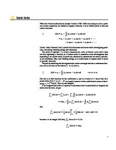
where T is the total time of flight and nr and nθ are the number of Fourier terms. Although there is no upper limit on the number of included Fourier terms (nr ≥ 2, nθ ≥ 2), the computational efficiency is an important consideration. The minimum number of 2 for Fourier terms is selected such that each Fourier approximation satisfies the BCs in the case of rendezvous. A discussion will follow in this paper in Section 2.4 on the appropriate values for nr and nθ for each type of trajectory. The governing equations of motion of a spacecraft in a two-body gravitational field can be written in the following polar forms using the Newton’s gravitational law [31]:     r¨ − rθ˙ 2 + µ2 = Ta sin (α ) r

(2.5)

   2˙rθ˙ + rθ¨ = Ta cos (α )

where, as shown in Fig.2.1(a), r is the magnitude of the position vector~r, v is the magnitude of the velocity vector ~v, θ is the polar angle, γ is the flight path-angle, α is the steering angle, Ta is the Thrust Acceleration(TA) magnitude, and µ is the gravitational parameter. In the 2-D trajectories, it is assumed that the thrust is aligned along or against the velocity

17

(a) Trajectory Variables

(b) Definition of angles

Figure 2.1: Nominal trajectory variables vector [27, 28, 20, 21, 31]. Thus, the thrust pointing angle α can be written as:

α = γ + nπ

(2.6)

where n is 0 or 1 for along or against the fight-path angle, respectively. From the second relation of Eq.(2.5) one can write:

2˙rθ˙ + rθ¨ 2˙rθ˙ + rθ¨ = Ta cos (α ) ⇒ Ta = cos (α )

(2.7)

Substituting the value for thrust acceleration into the first relation of Eq.2.5 one can write:



µ 2˙rθ˙ + rθ¨ r¨ − rθ˙ 2 + 2 = sin (α ) = 2˙rθ˙ + rθ¨ tan (α ) = 2˙rθ˙ + rθ¨ tan (γ ) r cos (α )

(2.8)

where the tangential thrust assumption can be written as:

tan (α ) =

r˙ rθ˙

(2.9)

18

Finally, one can derive one combined relation for EoM:




3 f (r, r˙, r¨, θ˙ , θ¨ ) = r2 θ˙ r¨ − r˙θ¨ + θ˙ µ − 2rr˙2 − rθ˙ = 0

(2.10)

The TA constraint (C) can also be written according to the following formula

Ta =

rθ˙ 2˙rθ˙ + rθ¨ ; cos (α ) = cos (γ ) = q
2 cos (α ) (˙r)2 + rθ˙  2 Ta C: ≤1 Ta,max

(2.11)

where Ta,max is the maximum allowed value for TA. Assuming specific values for nr and nθ , the FFS approximation is defined in terms of the unknown coefficients. The total number of unknowns are n = 2(nr + nθ + 1). The Fourier approximations for r and θ are constrained to satisfy the BCs. The BCs can be used to solve for some of the coefficients in terms of the rest of the coefficients. The selection of the specific coefficients, to be solved for, will affect the sensitivity of convergence. However, in this paper, the first eight coefficients are solved in terms of the rest of the coefficients for rendezvous problems, as they play important roles compared to low-order coefficients [35]. Appendix B.1 shows, for instance, how these constraints are used to derive relations between the coefficients in the rendezvous problem. Note that

θ f = θ0 + Nrev × 2π

(2.12)

19

The angle θ0 is the initial angle between ri and r f measured counterclockwise, as in Fig.2.1(b), and Nrev is the number of revolutions about the attracting central body. The value of Nrev is selected by trial and error in the test cases presented in this paper. In an optimization process, it can be one of the optimization parameters. Substituting the state approximations, Eqs.(2.3),(2.4) and (B.1) into Eq.(2.10), the differential equation is converted to a nonlinear algebraic equation, in which the only unknowns are the FFS coefficients and the independent time variable.

f (a0 , a1 · · · anr , b1 · · · bnr , c0 , c1 · · · cnθ , d1 · · · dnθ ;t) = 0

(2.13)

Suppose the number of unknown coefficients is n. Eq.(3.2) is true at all times, from the initial to the final times. In order to solve for the unknown coefficients, Eq.(3.2) will be computed at m points, called discretization points (DPs). We can write an equation at each of the DPs, to obtain m equations. There are generally several methods to solve the resulting nonlinear programming problem, given the constraints on TA.

Some nonlinear programming solvers minimize the summation of the squared residuals at all DPs, while other solvers find the exact solution if the system is square (number of equations is equal to the number of unknowns, n = m). In order to construct a square system, one should use a high number of terms in the Fourier series. Because the equations of motion are discretized at the DPs, the number of DPs should not be too low, in order to guarantee a feasible solution. The minimum number of DPs depends on the problem and

20

the duration of the maneuver. It is possible to figure out the minimum number of DPs for a specific problem after a few trials. Based on the cases presented in this paper, a safe choice of 10 points per revolution eliminates the need for trial and error. Also, the maximum number of terms in the FFS (after which no significant improvement in accuracy can be obtained) is determined by trial and error. However, the maximum number of FFS terms does not change much from one problem to another, as shown in the examples presented in this paper. Because the number of FFS terms is always less than the number of DPs, an over-determined system of equations is constructed (the number of equations is more than the number of unknowns, m > n).

For the rendezvous case the procedure can be summarized as follows. Given departure time, time of flight, Nrev , nr and nθ : (1) Compute the boundary values (ri , θi , r f , θ f , r˙i , θ˙i , r˙ f , θ˙ f ) using the terminal position and velocity vectors (2) Compute initial guesses for the unknown coefficients (a0 and c0 for the case with nr = nθ = 2) according to section 2.3. It should be noted that the number of unknown coefficients for this section is 2(nr + nθ ) − 6 since eight of the coefficients can be calculated enforcing the BCs, i.e. Eqs.(B.5), (3) Use Eqs.(B.5) to solve for eight of the coefficients using the coefficients from the previous step as well as boundary values, (4) Divide the time of flight into intervals and evaluate the equations of motion at the boundary points of these intervals to construct m algebraic nonlinear equations, (5) Divide the equation of constraint on thrust Eq.(3.1) according to the time discretization scheme to construct m equations, (6) Solve the resulting nonlinear programming problem (m equations), subject to the m constraint obtained in the previous

21

step. While the first m relations from the EoM are equalities the rest m relations from the constraint are inequalities. Therefore, there are 2m relations to be satisfied by the Fourier coefficients but m of them are inequalities. The minimum number of Fourier coefficients, nr and nθ , is problem dependent. The interesting feature of this method is that, once the time discretization is done, the cos and sine terms can be computed and stored once for the next iterations. This will help to reduce the computational time in constructing the equations. The case studies presented in this paper are from different categories of orbit maneuvers (rendezvous, orbit raising, and phasing). The value of nr and nθ presented in each of these examples may be considered as suggested values for all problems of the same category.

2.3 Initial Guess for Fourier Coefficients

The unknowns in the nonlinear programming problem are Fourier coefficients. Solving this nonlinear programming problem requires initial guesses for the coefficients. In the IP and exponential sinusoid SB methods, one of the states is transcribed in terms of the other states, e.g. r is represented as a function of θ . In the FFS method, the transcription of the states in terms of the independent variable time, makes it easier to calculate the initial guesses. To find a good initial guess, a simple shape is assumed for the trajectory and the corresponding Fourier coefficients for this shape are used as initial guesses. To efficiently provide this initial guess for the coefficients, two different categories of problems are considered: orbit 22

changing problems and phasing problems.

2.3.1 Orbit changing problems

For orbit changing problems, such as interplanetary transfers, the profile of the radius, r(t), increases (decreases), while the polar angle, θ (t), always increases. Two candidate functions can be used to represent r: the Tangent Hyperbolic(TH) function and the Cubic Polynomial(CP) function. For the TH approximation of r and θ , let:

   t − t0 1 (ar + br ) + (br − ar ) tanh r(t) = 2 ω

(2.14)

   1 t − t0 (aθ + bθ ) + (bθ − aθ ) tanh θ (t) = 2 ω

(2.15)

where ar = r0 , br = r f , aθ = θi , bθ = θ f ,t0 =

T and ω is a measure of the width of the 2

function and can change in the given range 1 ≤ ω ≤ 3 (in TU/rad) so as to provide reasonable gradual change. The TH provides a good approximation for the gradually changing r. The CP approximation can be used to represent both r and θ as follows:

r(t) = at 3 + bt 2 + ct + d

(2.16)

23

θ (t) = et 3 + f t 2 + gt + h

(2.17)

The BCs are used to compute all of the coefficients in Eqs.(2.16) and (2.17), as detailed in Appendix B.3.

2.3.2 Phasing problems

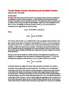
In a phasing maneuver, a spacecraft leaves its orbit and returns back to the same orbit, but phased, in order to rendezvous with another vehicle. Therefore, the final radius is the same as the initial one. Two jointed cubic polynomials are used for approximating the winding inside (or outside) orbits, as shown in Figure 2.2. Figure 2.2 shows the two possible phasing strategies: (i) increasing r, and then returning to the initial radius, and (d) decreasing r and then returning to the initial radius. In both strategies, the trajectory is divided into two segments: s1 and s2. The two segments meet at time tm , the time of maximum or minimum value of r, 0 < tm < t f .

rs1 (t) = as1

t3 + b

2 s1 t + cs1 t + ds1 ;



t∈ 0  3 2 rs2 (t) = as2t + bs2t + cs2t + ds2 ;t ∈ tm

tm tf





(2.18)

The coefficients in Eq. (2.18) can be computed from the BCs, as shown in Appendix B.4. For the polar angle (θ ) Eq.(2.17) is used.

24

i

S1(t)

t

m

rmax

S2(t)

d

r(t)

tm

t

f

i

S2(t) S1(t)

rmin d

t

Figure 2.2: Two jointed CPs approximation for r profile of the phasing problem

2.3.3 Coefficient calculations

Once the approximate functions for r and θ are computed, an initial guess for the Fourier coefficients is computed as follows. The approximate function for r(t) is evaluated at nr points, uniformly distributed in time.

r(ti ) =

                              

Ar T H (ti) or ArCP (ti )

; i = 0 · · · (nr − 1)

or A2CP r (ti )

25

(2.19)

where t0 = 0, tnr −1 = T and  nπ   nπ o nr n a0 r(ti ) = + ∑ an cos ti + bn sin ti 2 n=1 T T    1 ti − t0 TH Ar (ti ) = (ar + br ) + (br − ar ) tanh 2 ω ArCP (ti ) = ati 3 + bti 2 + cti + d     as1t 3 + bs1t 2 + cs1t + ds1 ; 0 ≤ t ≤ tm 2CP Ar =    as2t 3 + bs2t 2 + cs2 t + ds2 ; tm ≤ t ≤ t f

(2.20)

Similarly, the polar angle function is evaluated at nθ points:

θ (t j ) = Aθ CP (t j ) ; j = 0 · · · (nθ − 1)

(2.21)

where,

θ (t j ) =

 nπ o  nπ  c0 nθ n + ∑ cn cos t j + dn sin tj 2 n=1 T T

(2.22)

Aθ CP (t j ) = et j 3 + f t j 2 + gt j + h Using Eqs.(2.19) and (2.21) for r and θ one can form a set of linear equations and solve for the unknown coefficients with a simple matrix inversion for each one of the states, i.e. X = A−1 B, where matrix A, vector B, and calculation of the 2nr + 1 Fourier coefficients are discussed in Appendix B.5. This is the approach used to determine initial guesses for the coefficients to start the solver for both the constrained and unconstrained cases.

26

2.4 Test Cases

Four case studies for the application of the FFS method are presented in this section. The solutions are compared to the IP method solutions. For Earth to Mars transfer, canonical units are used such that 1 Distance Unit(DU) is 1 AU and 2 Time Unit(TU) is 1 year. For the rest of the problems, 1 DU is 1 earth radius and 1 TU is 806.8 sec. In each case, two FFS solutions are computed: one solution assumes no constraint on the thrust (UFF) and the second solution assumes a constraint on the TA value (CFF). For UFF and CFF problems, Matlab Fsolve and Fmincon functions are used respectively without any first or second order derivative information. Computational efficiency of the different algorithms are compared. The execution time, presented in the following case studies, includes the initialization of coefficients until convergence for the FFS, and the convergence for parameter d of the IP method. The difference between the time computation of both methods is important as the FFS method handles the trajectory and TA constraint explicitly while the IP method does it implicitly. Therefore, once the FFS solver converges the trajectory is totally defined while for the IP method the convergence defines the total coefficients of the shape and the trajectory needs to be constructed. The computational efficiency of the FFS method is independent of the coefficients initialization function (TH or CP). All of the test cases have been performed on an Intel Xeon Pentium 4 1.86 GHz with Windows XP. There are some points worth noting. This method does not provide a solution to any thrust level that is defined as a constraint. Thus, if a solution exists, the FFS 27

method finds it in a reasonable time. However, if a solution does not exit, the constraint FFS method needs more time to confirm that there is no solution. This drawback can be overcome by defining a maximum number of iterations for the solver.

2.4.1 Earth-Mars transfer

The Low-thrust Earth-Mars transfer is considered. A spacecraft is transferred from the Earth to rendezvous with Mars, given TA limitations [40]. The BCs and input parameters are listed in Table 3.1. Figure 2.3 also shows the solution trajectories for the unconstrained, Table 2.1 Input parameters and boundary conditions for Earth-Mars problem BCs ri = 1(DU ) θi = 0 (rad) r f = 1.5234 (DU) θ f = 9.831 (rad) r˙i = 0 (DU/TU) θ˙i = 1 (rad/TU) r˙ f = 0 (DU/TU) ˙ θ f = 0.5318 (rad/TU)

Input Parameters Nrev = 1 nr = 2 nθ = 5 Isp = 5.9728 × 10−4 (TU ) Ta,max = 0.02 (DU /TU 2 ) # of DPs = 22 T = 13.447 (TU)

constrained, and the IP method. Figure 2.4 shows the TA history for the three methods. As shown in Figure 2.4, the CFF was able to find a trajectory that satisfies the TA constraint; the constrained trajectory resembles the FFS unconstrained solution in many parts of the trajectory. The IP solution has a TA history that starts and ends at low levels and increases to its maximum magnitude at about mid course of the total flight time; this is a typical

28

profile for the TA obtained from the IP method. 1.5 1 Earth orbit

Y (DU)

0.5

Mars Orbit Constrained FF

0

IP Departure point Arrival point

−0.5

Unconstrained FF

−1 −1.5 −1.5

−1

−0.5

0 X (DU)

0.5

1

1.5

Figure 2.3: Earth to Mars trajectory

Ta (DU/TU2)

0.033 0.03

UFF IP CFF

0.02

0.01

0

0

5

10 t (TU)

Figure 2.4: Earth to Mars thrust profile

Two parameters affect the accuracy of the solution: the number of DPs and the number of terms in the FFS. The distribution of discretization points is selected to be uniform in time. The computational performance in terms of time for CFF and IP methods are 0.08 and 0.11 seconds, respectively where the number of descetization points per revolution is NDP = 11 and the total DPs is calculated according to (Nrev + 1)NDP which results in 22 DPs. If

29

the number of DPs is less than 15, it will not be possible to fully capture the trajectory topologies and the solver does not converge. If the number of DPs is more than 80 points, no better accuracy is attained due to an increase in the residuals. It has been observed that increasing the number of FFS terms, up to a limit, improves the solution accuracy. Beyond this limit, the accuracy may be degraded because of the round off errors. For the IP method, the initial value of d is set to zero as it was suggested in [31]. It is noted that, for the sake of comparison with the IP method, the value of the TA constraint is selected such that the IP solution violates it. In this example, it was found that the minimum thrust acceleration level for which there exists a solution is 0.017 DU /TU 2 .

2.4.2 LEO to GEO orbit transfer (rendezvous)

The transfer maneuver from a low-Earth circular orbit to a geostationary circular orbit is considered. The initial and final radii are: ri = 6, 570 Km and r f = 42, 160 Km [41]. The original finite burn problem, solved in a Cartesian coordinate system, has a total time of flight of about 120, 000 seconds [41]. The practical LEO to GEO orbit transfer problem is an orbit raising problem, in which the final value of the polar angle, θ f , is free. Shape based methods such as IP and exponential sinusoid methods cannot handle this problem in its general form; SB methods can only solve rendezvous problems. For the sake of comparing the FFS method to the IP method, a final value for the polar angle, θ f , will be assumed in this section. In section 2.4.3, the orbit raising problem will be solved using

30

FFS. In this section, we will fix the final value of the polar angle by assuming θ0 = π . The problem becomes a rendezvous-like problem. Reference [31] presents two shape-based IP methods. One of them is the 7th degree IP method and is used to solve rendezvous problems, with a fixed time of flight. The other method is a 6th degree IP method and it solves time free rendezvous maneuvers.

Assuming that the time of flight for the LEO to GEO transfer is 120, 000 seconds [41], and applying the 7th degree IP method to solve the problem, results in a trajectory that intersects the earth’s surface. The solution from the 7th degree IP method is shown in Figure 2.5 where the trajectory winds inside the Earth surface. Figure 2.6 shows the thrust profile for this non-feasible solution. The 6th degree IP method is used to solve the time free version of this problem. The obtained solution performs 7 revolutions and has a total flight time of 206, 331.4 seconds. The trajectory and the TA history are also shown in Figures 2.5 and 2.6.

6 4

Y (DU)

2 0 −2 −4 −6 −8

6th Degree IP LEO GEO 7th Degree IP

−10

−5

0

5

X (DU)

Figure 2.5: LEO to GEO trajectories using IP methods

31

0.04 7th degree IP 6th degree IP

0.03

Ta (DU/TU2)

0.02 0.01 0 −0.01 −0.02 −0.03 0

50

100

150 t (TU)

200

250

300

Figure 2.6: TA profiles for the LEO to GEO trajectories using IP methods The FFS method is implemented in this LEO to GEO transfer problem. The input parameters and BCs are listed in Table 3.2, where the value of θ f corresponds to θ0 = π . The time of flight is assumed to be 120, 000 seconds. Table 2.2 Input parameters and boundary conditions for the LEO-GEO problem BCs ri = 1.0313 (DU) θi = 0 (rad) r f = 6.61 (DU) θ f = 47.123 (rad) r˙i = 0 (DU/TU) θ˙i = 0.95652 (rad/TU) r˙ f = 0 (DU/TU) θ˙ f = 0.058842 (rad/TU)

Input parameters Nrev = 7 nr = 2 nθ = 3 Isp = 3.7183 (TU) # of DPs = 40 Ta,max = 0.0153 (DU /TU 2 ) T = 148.73 (TU)

Two cases are solved: no constraint on the thrust acceleration, and thrust acceleration is constrained to be less than Ta,max = 0.15m/s2 = 0.0153DU /TU 2 .

The trajectories and TA for both the unconstrained and constrained solutions are depicted in

32

0.02

2

Ta (DU/TU )

0.01 0 −0.01

CFF UFF

−0.02 −0.03 0

Ta,max 50

100

150

t (TU)

Figure 2.7: LEO to GEO TA profile using FFS method

6 4

Y (DU)

2 0 −2 −4 −6 −8

Unconstrained FF LEO GEO Constrained FF −10

−5

0

5

X (DU)

Figure 2.8: LEO to GEO trajectory profile using FFS method Figures 2.7 and 2.8. As it can be seen, the thrust constraint is active at the final point of the CFF solution. The UFF TA profile in general looks pretty similar to the CFF method. The distances from Earth for both solutions are also depicted in Figure 2.9. The two solutions (unconstrained and constrained thrust acceleration) do not intersect the earth’s surface, however, only the constrained version satisfies the TA constraint. For the Earth-bounded problems, there is no clear way for guessing an initial value for the d parameter in the IP method. Thus, three different values for d were tested in this problem. The computational 33

7 6

Unconstrained FF Constrained FF

r (DU)

5 4 3 2 1 0

50

100

150

t (TU)

Figure 2.9: LEO to GEO radius profile using FFS method performance of CFF method is 0.06 seconds. Starting the IP d parameter with a zero value leads to no convergence and the computational time for different initial d values of 0.001 and 3.5e-4 is 0.06 and 0.03 seconds respectively. The positive and negative values for the TA correspond to acceleration and deceleration situations. It is also important to take it into consideration that during the initial guess construction for a direct solver the direction of the TA vector is against the velocity vector for negative values of TA. The switching TA profile is another point worth noting. Since both the constrained and unconstrained versions of the problem show switching, it is not due to the TA constraint enforcement. A better explanation can be given in view of the results plotted in Figure 2.6. It is interesting to note that the seventh degree IP also results in negative values of TA for considerable amount of time during the initial phase of transfer which is counter intuitive and is a direct consequence of the time constraint ( in the rendezvous case) as well as the assumed shape to the extent that makes the resulted transfer trajectory infeasible. However, this phenomenon

34

is not observed in the sixth degree IP due to the freedom in the time of flight. For the constrained finite Fourier series the switching of TA profile happens at a bigger time and since the TA profile is increasing at the beginning of the transfer there is no encounter with the Earth surface. In fact, for this example if the time of flight is approximately bigger than 177000 seconds no TA profile switching is observed. Therefore, the time of flight constraint in the root cause for switching of the thrust acceleration.

35

2.4.3 LEO to GEO orbit raising

The FFS method can also handle problems with free arrival angle, θ f , as in the orbit-raising problems. The FFS algorithm, presented in section 2.2, will be used with a minor change. Because the final angle, θ f , is free, no boundary condition can be applied on θ f . Hence, the number of Fourier coefficients that can be computed from BCs reduces from eight to seven. The list of the seven coefficients and their expressions are listed in Appendix B.2. This adds one more unknown to the unknown coefficients that are computed from the equations of motion evaluated at the DPs; without affecting the solution algorithm of the nonlinear programming problem. To generate the initial guess for the coefficients, an approximate guess for the final value of the polar angle is assumed: θ f = 2π × Nrev (this is equivalent to θ0 = 0.) Note that this is merely an initial guess for θ f for the initialization scheme. 0.015 0.01

2

Ta (DU/TU )

0.005 0

CFF UFF

−0.005 −0.01 −0.015 Ta,max −0.02 −0.025 0

50

100

150

t (TU)

Figure 2.10: LEO to GEO raising using FFS method - TA profile

36

8

UFF LEO GEO CFF

6 4 Y (DU)

2 0 −2 −4 −6 −8 −10

−5

0 X (DU)

5

10

Figure 2.11: LEO to GEO raising using FFS method - Trajectory

7 6

r (DU)

5

UFF CFF

4 3 2 1 0

50

100

150

t (TU)

Figure 2.12: LEO to GEO raising using FFS method - radius profile

50

θ (rad)

40 CFF UFF

30 20 10 0 0

50

100

150

t (TU)

Figure 2.13: LEO to GEO raising using FFS method - polar angle profile

37

For this LEO to GEO orbit-raising problem, both the unconstrained and the constrained (Ta,max = 0.0102 (DU /TU 2 )) cases are solved using the FFS method. The problem BCs are the same as those in Table 3.2, except for θ f , which is now free, and for the number of Fourier terms. For the coefficients initialization of both CFF and UFF versions, the cubic polynomial is used as the approximation profile for both the radius and the polar angle. The total number of DPs is equal to 40. Figure 2.10 shows the TA profile for both cases. Again the switching TA profile is a consequence of the fixed time of flight constraint and it was explained in the previous test case. The trajectories of both cases are shown in Figure 2.11. Figures 2.12 and 2.13 show that the UFF and the CFF solutions are identical when the radius and the polar angle are plotted as functions of time. As it is shown the CFF method was capable of finding a satisfactory solution. In addition, the TA profiles of both UFF and CFF methods are similar to each other except for the last segment of the trajectory as shown in Figures 2.10. The final polar angle (θ f ) is 41.76 degrees. In addition, results show that the UFF solution has the capability to be used as an initial guess for the CFF method.

2.4.4 LEO Phasing Maneuver

The FFS method is applied to two phasing problems. In both problems, the spacecraft is in a 200 km altitude orbit. The required phasing, between initial and final positions, is 90o in one case, and is 180o in the other case. This problem is of a practical importance. Because

38

of the low altitude, some solution trajectories that attempt to go to a lower altitude for phasing may go below the Earth radius and are obviously infeasible. In addition, phasing maneuver problems differ from the other cases in that the radius returns to its initial value after, in general, multiple revolutions. Hence, the radius, r, does not follow a monotonically increasing or decreasing change. To provide a good initial guess for the FFS coefficients, in this category of problems, the initial guess trajectory is assumed to take the shape of two jointed cubic polynomials, as detailed in section 2.3. The problem BCs and input parameters are listed in Table 3.3. For both cases the following parameters are common: Nrev = 1, Isp = 3.7183(TU ), nr = 3, nθ = 6. The solution results for the FFS and the IP Table 2.3 Input parameters and BCs for the phasing problem: FFS and IP mehtods Parameters & BCs

Value 180o 0.0204 0.0051 60 60 8.924 10.262 1.0313 1.0313 0 0 0 0 0.9548 0.9548 1.0313 1.0313 0 0 7.8539 7.8539 0.9548 0.9548 90o

Ta,max (DU /TU 2) # of DPs T (TU) ri (DU) r˙i (DU/TU) θi (rad) θ˙i (rad/TU) r f (DU) r˙ f (DU/TU) θ f (rad) θ˙ f (rad/TU)

methods are shown in Figures 2.14 and 2.15 for the 90o phasing, and in Figures 2.16 and 2.17 for the 180o phasing.

39

1

Y (DU)

0.5

IP Trajectory Earth Surface Departure Point Arrival Point UFF CFF LEO (h=200 km)

0

−0.5

−1 −1

−0.5

0 X (DU)

0.5

1

Figure 2.14: Phasing trajectory - 90o phasing

0.06 IP UFF CFF

0.04

2

Ta (DU/TU )

Ta,max 0.02 0 −0.02 −0.04 −0.06 0

2

4 t (TU)

6

8

Figure 2.15: Phasing thrust profile - 90o phasing Clearly, the FFS solution is able to satisfy the thrust constraint in both phasing cases. From Figures 2.15 and 2.17, we can see that the unconstrained thrust profile resembles two accelerations near the beginning and the end of the phasing mission, while almost coasting during the rest of the trajectory. Adding the TA constraint increases the fluctuations in the thrust during the course of the flight time.

40

1

Y (DU)

0.5

IP Trajectory Earth Surface LEO (h=200 km) Departure Point Arrival Point UFF CFF

0 −0.5 −1 −1

−0.5

0

0.5

1

X (DU)

Figure 2.16: Phasing trajectory - 180o phasing

0.04 IP UFF CFF

0.03 Ta,max

0.01

2

Ta (DU/TU )

0.02

0 −0.01 −0.02 −0.03 −0.04 0

2

4 6 Time (TU)

8

10

Figure 2.17: Phasing thrust profile - 180o phasing

2.5 Conclusions

A new method is developed to provide feasible low-thrust trajectories based on using the finite Fourier series to approximate the shape of the trajectories inversely. The new method can handle constraints on the maximum thrust acceleration. Shape based methods typically assume a fixed shape for the trajectory. This method, however, does not assume a specific

41

shape for the trajectory. Rather, it assumes an approximation for the trajectory shape in terms of finite fourier series expansion of states. For every different selection of the Fourier coefficients, a different shape is obtained. Hence, it was possible to handle the thrust acceleration constraint by searching for the Fourier coefficients that represent a solution that satisfies the constraints. The ability of this method to solve problems with a greater number of free parameters than shape-based methods seems to be a key point. In addition, it can handle problems in both weak and strong gravity fields i.e. low Earth and interplanetary transfers as it was shown in test cases.

In the absence of thrust acceleration constraints, the computational time of the FFS method is observed to be in the same order of magnitude as the inverse polynomial shape-based method. When thrust acceleration constraints are imposed, the computational time of the FFS method depends on the existence of the solution. If a solution exists, the FFS method finds it in about the same time as the unconstrained FFS method. If a solution does not exist, the constraint FFS method needs more time to confirm that there is no solution.

42

Chapter 3

Fourier Series for Modulated Thrust

3.1 Introduction

In this chapter1 , based on the previously introduced concept of Finite Fourier series a new capability of thrust modulation for trajectory generation is sought. The solutions are of near thrust arcs and non-thrust arcs trend. In addition, the resulting solutions are good initial guesses for direct optimization techniques. Few case studies are presented: simple Earth-Mars rendezvous, LEO-to-GEO rendezvous, and phasing problems. Results, clearly depict the capability of this method for modulated thrust profile solutions.

The FFS representation and discretization strategy has already been introduced in section 1 The

material of this chapter are copied in whole from Reference [42]

43

2.2. The use of FFS and discretization notions reduces the problem to a system of algebraic equations in the FFS coefficients. However, the TA constraint is dealt with another approach and section 3.3 explains it. Section 3.3 presents applications of the proposed method on various 2-D problems. It compares results with other methods in the literature, and shows details of the resulting trajectories in terms of thrust acceleration profile, trajectory shape.

3.2 Problem Formulation

The approach to handle TA constraint (C) is different from the previous paper in the manner that it is translated to equality constraints and instead we are looking for the slack variables such that they satisfy the thrust constraint. In essence the constraint can be written according to the following formula

Ta =

2˙rθ˙ + rθ¨ rθ˙ ; cos (α ) = cos (γ ) = q
2 cos (α ) (˙r)2 + rθ˙ C:

Ta

Ta,max

(3.1)

+ σi = 1

where Ta,max is the maximum allowed value for TA and σi is the slack variable to be determined and can take on values from 0 to 2 corresponding to different thrust values of Ta,max , 0 and −Ta,max respectively.

44

Substituting the state approximations, Eqs.(2.3),(2.4) and (B.1) into Eq.(2.10), the differential equation is converted to a nonlinear algebraic equation, in which the only unknowns are the FFS coefficients and the independent time variable.

f (a0 , a1 · · · anr , b1 · · · bnr , c0 , c1 · · · cnθ , d1 · · · dnθ ;t) = 0

(3.2)

The same is true for Eq.(3.1) with the addition of slack variables:

C (a0 , a1 · · · anr , b1 · · · bnr , c0 , c1 · · · cnθ , d1 · · · dnθ ;t; σi) = 0

(3.3)

Here the slack variables are forced to take on the different prescribed values. Suppose the number of unknown coefficients is n. Eq.(3.2) is true at all times, from the initial to the final times. In order to solve for the unknown coefficients, Eq.(3.2) will be computed at m points, called discretization points (DPs). For the TA constraint i.e. Eq.(3.2) we will divide the whole time into some intervals. At each interval, the values of σ ′ s are equal to each other. By doing so, we will decrease the number of slack variables and this makes the execution time lesser. The schematic graph of a three interval thrust profile is shown in Figure 3.1. It is important to note that at each interval the sigma’s are equal to each other and in the provided figure there are only 3 slack variables to be determined and the other slack variables are assigned based on the interval they are at. We can write an equation at each of the DPs, to obtain m equations. There are generally several methods to solve the resulting Mixed-Integer nonlinear programming problem.

45

Figure 3.1: Three interval schematic view of thrust profile and slack variables

3.3 Test Cases

Three case studies for the application of the Modulated FFS method are presented in this section. For Earth to Mars transfer, canonical units are used such that 1 Distance Unit(DU) is 1 AU and 2 Time Unit(TU) is 1 year. For the rest of the problems, 1 DU is 1 earth radius and 1 TU is 806.8 sec. We have use Tomlab Matlab optimization toolbox for solving all of the cases. All of the test cases have been performed on an Intel Xeon Pentium 4 1.86 GHz with Windows XP. There are some points worth noting. This method does not provide a solution to any thrust level that is defined as a constraint.

46

3.3.1 Earth-Mars transfer

The Low-thrust Earth-Mars transfer is considered. A spacecraft is transferred from the Earth to rendezvous with Mars, given TA limitations [40]. The BCs and input parameters are listed in Table 3.1. Figure 3.2 also shows the solution trajectory. Figure 3.3 shows the Table 3.1 Input parameters and boundary conditions for Earth-Mars problem BCs ri = 1(DU ) θi = 0 (rad) r f = 1.5234 (DU) θ f = 9.831 (rad) r˙i = 0 (DU/TU) θ˙i = 1 (rad/TU) r˙ f = 0 (DU/TU) θ˙ f = 0.5318 (rad/TU)

Input Parameters Nrev = 1 nr = 20 nθ = 20 Isp = 5.9728 × 10−4 (TU ) Ta,max = 0.02 (DU /TU 2 ) # of DPs = 22 T = 13.447 (TU)

respected TA history. 1.5 1

Y (DU)

0.5 Earth Orbit transfer trajectory Mars Orbit

0 −0.5 −1 −1.5 −1.5

−1

−0.5

0 X (DU)

0.5

1

1.5

Figure 3.2: Earth to Mars trajectory

47

0.025

Ta (DU/TU2)

0.02 0.015 0.01 0.005 0 −0.005 0

5

10

15

t (TU)

Figure 3.3: Earth to Mars thrust profile Two parameters affect the accuracy of the solution: the number of DPs and the number of terms in the FFS. The distribution of discretization points is selected to be uniform in time. The number of descetization points per revolution is NDP = 11 and the total DPs is calculated according to (Nrev + 1)NDP which results in 22 DPs. If the number of DPs is less than 15, it will not be possible to fully capture the trajectory topologies and the solver does not converge. If the number of DPs is more than 80 points, no better accuracy is attained due to an increase in the residuals. It has been observed that increasing the number of FFS terms, up to a limit, improves the solution accuracy. Beyond this limit, the accuracy may get degraded because of the round off errors.

3.3.2 LEO to GEO orbit transfer (rendezvous)

The transfer maneuver from a low-Earth circular orbit to a geostationary circular orbit is considered. The initial and final radii are: ri = 6, 570 Km and r f = 42, 160 Km [41]. The

48

original finite burn problem, solved in a Cartesian coordinate system, has a total time of flight of about 120, 000 seconds [41]. The practical LEO to GEO orbit transfer problem is an orbit raising problem, in which the final value of the polar angle, θ f , is free. In this section, we will fix the final value of the polar angle by assuming θ0 = π . The problem becomes a rendezvous-like problem. The Modulated thrust FFS method is implemented in this LEO to GEO transfer problem. The input parameters and BCs are listed in Table 3.2, where the shown value of θ f corresponds to θ0 = π . The time of flight is assumed to be 120, 000 seconds. Table 3.2 Input parameters and boundary conditions for the LEO-GEO problem BCs ri = 1.0313 (DU) θi = 0 (rad) r f = 6.61 (DU) θ f = 47.123 (rad) r˙i = 0 (DU/TU) θ˙i = 0.95652 (rad/TU) r˙ f = 0 (DU/TU) θ˙ f = 0.058842 (rad/TU)

Input parameters Nrev = 7 nr = 20 nθ = 30 Isp = 3.7183 (TU) # of DPs = 40 Ta,max = 0.0153 (DU /TU 2 ) T = 148.73 (TU)

the thrust acceleration is constrained to be less than Ta,max = 0.15m/s2 = 0.0153DU /TU 2.The trajectories and TA for solutions are depicted in Figures 3.4 and 3.5.

49

−3

6

x 10

5

Ta (DU/TU2)

4 3 2 1 0 −1 0

50

100

150

t (TU)

Figure 3.4: LEO to GEO thrust acceleration profile using FFS method 8 Transfer trajectory LEO orbit GEO orbit

6

Y (DU)

4 2 0 −2 −4 −6 −8 −10

−5

0 X (DU)

5

10

Figure 3.5: LEO to GEO trajectory profile using FFS method

3.3.3 LEO Phasing Maneuver

The on/off thrust FFS method is applied to the phasing problem. The spacecraft is in a 200 km altitude orbit. The required phasing, between initial and final positions, is 90o [43]. Because of the low altitude, some solution trajectories that attempt to go to a lower altitude for phasing may go below the Earth radius and are obviously infeasible. The problem BCs and input parameters are listed in Table 3.3. In addition: Nrev = 1, Isp = 3.7183 (TU ), 50

nr = 6, nθ = 30. The solution results are shown in Fig. 3.6 and in Fig. 3.7. Table 3.3 Input parameters and BCs for the phasing problem Parameters & BCs Ta,max (DU /TU 2) # of DPs T (TU) ri (DU) r˙i (DU/TU) θi (rad) θ˙i (rad/TU) r f (DU) r˙ f (DU/TU) θ f (rad) θ˙ f (rad/TU)

Value 0.0204 60 8.924 1.0313 0 0 0.9548 1.0313 0 7.8539 0.9548

1

Y (DU)

0.5

Phasing orbit LEO orbit

0

−0.5

−1 −1

−0.5

0 X (DU)

0.5

1

Figure 3.6: Phasing trajectory - 90o phasing

51

0.04 0.03

T (DU/TU2)

0.02 0.01

a

0 −0.01 −0.02 −0.03 0

2

4

6

8

10

t (TU)

Figure 3.7: Phasing thrust profile - 90o phasing

3.4 Conclusions

A new method is developed to provide feasible low-thrust trajectories based on using the finite Fourier series to approximate the shape of the trajectories inversely. Besides the fast construction of space trajectories that satisfy given thrust constraints, the proposed method has the capability of generating on/off thrust profiles. This was possible by forcing the constraint slack variables to take only one of three discrete values. The three test cases presented in this Note demonstrated this capability. The drawback is that the computational time of the proposed on/off thrust finite Fourier series trajectory approximation is 3 to 4 orders of magnitude higher than that of the original finite Fourier series trajectory approximation method.

52

Chapter 4

Finite Fourier Series: Three-dimensional

4.1 Introduction

The main contribution of this chapter is the extension of the FFS approximation to the three-dimensional (3D) dynamic models 1 . In addition, a general reduced Fourier representation of the states and their associated derivatives is derived which diminishes the computational intensity. The proposed method provides initial trajectory guess that satisfies thrust constrains, the EoM, and the problem BCs. In essence, BCs are used to

1 The

material of this chapter will be submitted to the AIAA Journal of Spacecraft and Rockets

53

evaluate some of the FFS coefficients. The fourier approximation of the states are used to calculate the thrust acceleration inversely. The resulting thrust acceleration is evaluated at equally space distributed points in time to make a set of thrust acceleration constraints. The objective is to minimize ∆V , which is calculated through numerical integration of the thrust acceleration over time. Therefore, the problem converts to a NLP problem with Fourier coefficients as the unknown parameters.

The chapter is organized as follows. In section 4.2, the theory, EoM, objective function and TA constraints are explained. In addition, the initial FFS representation (and its reduced form) for the states is presented. The use of FFS and discretization notions reduces the problem to a system of algebraic equations in the FFS coefficients. A brief description of the overall problem along with the definition of independent and dependent design variables are given in sections 4.2.3. An efficient technique for the initialization of the unknown Fourier coefficients are explained in Section 4.3. Application of the proposed method on several missions is investigated is section4.4. Finally, section 4.5 presents a conclusion of the chapter.

4.2 Finite Fourier Series Method

In general, any periodic function can be written in terms of an infinite sum of sine and cosine functions (Fourier series). If Fourier representations of two different functions

54

are considered, the only difference is in the coefficients of the sine and cosine functions and perhaps the number of terms in the Finite Fourier Series (FFS). In this paper, it is suggested that a 3D trajectory shape is approximated by a FFS, with enough terms (free coefficients), rather than a fixed shape function which is a common practice among the existing SB methods. The coefficients in a FFS representation will not only satisfy the BCs, the EoM, and any other constraints such as TA constraints, but also they can be varied to represent different solutions and different trajectory shapes. The following sections explain the details of the solution procedure.

4.2.1 Coordinate System and Equations of Motion

Cylindrical coordinates are considered as the reference coordinate system mainly due to the fact that the dynamic EoM are simpler and involve fewer nonlinear terms compared to other coordinate systems. In addition, the polar and radial coordinates make the 3D approach quite similar to its planar two dimensional counterpart. The EoM in the cylindrical coordinates are as follows:

r¨ − rθ˙ 2 +

µ r = fr s3

(4.1)

rθ¨ + 2˙rθ˙ = fθ

(4.2)

55

z¨ +

µ z = fz s3

where s =

√

(4.3)

r2 + z2 ,µ is the gravitational parameter of the central body. fr , fθ and fz are

the thrust acceleration components of the low-thrust engine.

The construction of Fourier series and their associated derivatives is explained in section 4.2.2. Substituting the states and their respective first- and second-order derivatives into the left hand side of the EoM (Eq.(4.1),(4.2) and (4.3)), the required thrust acceleration along any coordinate can be computed. Then, the overall required thrust acceleration, Ta ,can be computed:

Ta =

q

fr 2 + fθ 2 + fz 2

(4.4)

In addition, the required total ∆V can be computed by numerical integration of the thrust acceleration over time:

∆V =

ZT

(4.5)

Ta dt

0

56

4.2.2 States Fourier Approximation

There are two options for approximating the trajectory shape. The first is to assume the states as a function of the polar angle θ , and expand this function using a FFS. The second option is to assume the approximation functions in the time domain. In this paper, the second option is adopted to avoid the introduction of extra constraint for time of flight. The physical position and velocity BCs are handled more efficiently in the time domain. In this paper, the cylindrical coordinates, radius, r, polar angle, θ and the axial coordinate, z, are approximated with Finite Fourier Series (FFS) as follows:

nr a0 r(τ ) = + ∑ {an cos(nπτ ) + bn sin(nπτ )} 2 n=1

(4.6)

c0 nθ + ∑ {cn cos(nπτ ) + dn sin(nπτ )} 2 n=1

(4.7)

θ (τ ) =

nz e0 z(τ ) = + ∑ {en cos(nπτ ) + fn sin(nπτ )} 2 n=1

where 0 ≤ τ =

t T

(4.8)

≤ 1 is the scaled time, T is the corresponding time of flight, nr and nθ

and nz are the number of Fourier terms (sum of sin and cos) for each state. The time of flight of is scaled to make the required discretization strategy (which is one of the steps of the solution procedure) independent of the time. In its general form, the Fourier series

57

approximations for r, θ and z are constrained to satisfy twelve rendezvous BCs

ri = r (τ = 0)

r f = r (τ = 1)

r′ i = r′ (τ = 0)

r′ i = r′ (τ = 1)

θi = θ (τ = 0)

θ f = θ (τ = 1)

θ′

θ′

i

θ ′ (τ

=

= 0)

f

= θ ′ (τ

(4.9)

= 1)

zi = z (τ = 0)

z f = z (τ = 1)

z′ i = z′ (τ = 0)

z′ f = z′ (τ = 1)

The prime denotes derivative with respect to the scaled time, τ , and subscripts "i" and "f" denote the initial and final conditions respectively. The relations between the time and scaled-time first and second derivatives are

d dt d2 dt 2

=

1 d T dτ

=

(4.10)

1 d2 T 2 dτ 2

Therefor, the twelve BCs can be related according to the following relations

ri = ri

rf = rf

r′ i = T r˙i

r′ f = T r˙ f

θi = θi

θf = θf

θ ′ i = T θ˙i

θ ′ f = T θ˙ f

zi = zi

zf = zf

z′ i = T z˙i

z′ f = T z˙ f 58

It is important to note that twelve BCs are associated with a rendezvous problem and it is advantageous to remove as much unknown Fourier coefficients as possible from the unknowns. The main reason of such strategy is that the BCs are physical meaningful quantities in contrast to the Fourier coefficients. In fact, the direct approximation of Fourier coefficients is not straightforward because the relation between the resulted value of the Fourier approximation of different frequencies is not evident. Therefore, it is easier and more physically meaningful to extract some of the unknown Fourier coefficients in terms of the physical sensible values and reduce the number of design variables. In general, this strategy does not affect the entirety of the problem whereas the physically meaningful BCs can be considered as design variables.

In this work, the first four Fourier coefficients (excluding the first constant number) of each approximation are derived in terms of the known BCs and the rest of the coefficients hence nr ≥ 2, nθ ≥ 2 and nz ≥ 2. To express which one of the coefficients in terms of the others will affect the sensitivity of convergence as the first coefficients play important roles compared to low-order coefficients [35]. For example, considering the four BCs on radius (ri , ri′ , r f , r′f ), four of the coefficients (a1 , b1 , a2 , b2 ) can be computed in terms of the given BCs and other coefficients. If these four coefficients are substituted into the Eq.(5.13) and rearranged, the radius Fourier approximation function can be written in the following reduced form:

nr

r(τ ) = Fr +Ca0 a0 + ∑ {Can an +Cbn bn } n=3

59

(4.11)

where the BCs appear only in term Fr and is a fixed vector for rendezvous problems. The equations for different terms and coefficients of the unknown parameters in Eq. (5.17) are

Fr =

1 2




ri − r f cos (πτ ) + 21π r′ i − r′ f sin (πτ ) + 21 ri + r f cos (2πτ )


+ 41π r′ i + r′ f sin (2πτ )

Ca0 = 21 [1 − cos (2πτ )]     cos(nπτ ) − cos(πτ ); Can =    cos(nπτ ) − cos(2πτ );     sin(nπτ ) − n sin(πτ ); Cbn =    sin(nπτ ) − n sin(2πτ ); 2

odd

(4.12)

even odd even

As can be seen, the coefficients of the unknown Fourier parameters (Can and Cbn ; n = 3 · · · nr ) depend on the discretization of the scaled-time variable ,τ , and can be used for reducing the computation time. Likewise, for the other two coordinates (θ and z) and their associated first and second τ -derivatives similar equations can be written (see Appendix C.1).

4.2.3 Problem description

The overall problem is to find a feasible low-thrust trajectory within the existing TA capability of the on-board propulsion system of a spacecraft. Equations. (4.1), (4.2) and (4.3) are true at all times. However, numerical integration is required for calculating total

60

∆V and it is required to evaluate the TA constraint at some discrete points. To solve for the unknown Fourier coefficients, each one of the thrust acceleration equations will be computed at m Discretization Points (DPs). The DPs are calculated according to the following relation

m = (Nrev + 1) × ppre

(4.13)

where Nrev is the number of revolutions and ppr is the corresponding points per revolution. For the current study Legendre-Gauss distribution of DPs is adopted,

τ0 = 0 < τ1 < · · · < τm−1 = 1

(4.14)

Because the EoM are discretized at the DPs, the number of DPs should not be too low, in order to guarantee a feasible smooth solution. The minimum number of DPs depends on the problem and the duration of the maneuver. It is also possible to figure out the minimum number of DPs for a specific problem after a few trials. It is also assumed that these DPs are fixed throughout the overall optimization. Since the number of DPs is fixed and the scaled-time vector is represented as a column vector, states and their associated first and second τ -derivatives can be written in a compact matrix notation form (See Appendix D.2). For instance r becomes

[r]m×1 = [Ar ]m×(2nr −3) [Xr ](2nr −3)×1 + [Fr ]m×1

61

(4.15)

where

[Ar ]m×(2nr −3) =

"

[Xr ](2nr −3)×1 =



Ca0 a0

Ca3 a3

Cb3 b3

Ca4 ···

and [Fr ] is defined in Eq. (5.18).

anr

Cb4 bnr

···

Canr

Cbnr

T

#

m×(2nr −3)

(4.16)

Altogether, for all of the states and their

associated τ -derivatives the coefficient matrix of the unknown Fourier coefficients ([Ar ] , [Ar′ ] , [Ar′′ ] , [Aθ ] , [Aθ ′ ] , [Aθ ′′ ], [Az ] , [Az′ ] , [Az′′ ]) are computed and will be stored once for later use in the solver for the evaluation of the objective functions and constraints. It should be noted that the BCs are fixed and no update of the F() vectors of the states and their associated derivatives is needed i.e. Fr , Fr′ , Fr′′ , Fθ , Fθ ′ , Fθ ′′ , Fz , Fz′ , Fz′′ .

In addition, once the number of Fourier terms (nr ) and Discretization Points (DPs) are determined the coefficient terms (Ca0 ,Ca3 ,Cb3 , · · · ,Canr ,Cbnr ) (see Appendix D.2) become fixed. These coefficients also can be calculated and stored once to enhance the computational efficiency. They also make the calculation of objective and constraints gradients easy.

Note that sin(πτ ), sin(2πτ ), cos(πτ ) and cos(2πτ ) appear in the

coefficients of the unknown parameters of the compact forms of states i.e. r(τ ) ,θ (τ ) and z(τ ) (see Appendix D.2).

The thrust acceleration equations can be written, using the matrix notation form of the

62

states and their associated first and second derivatives, in the following form,

[ fr ] = fr (Xr , [r] , [r′′ ] , [θ ′ ] , [z] , [z′′ ]) [ fθ ] = fθ (Xθ , [r] , [r′ ] , [θ ′ ] , [θ ′′ ])

(4.17)

[ fz ] = fz (Xz , [r] , [z] , [z′′ ]) likewise the thrust acceleration Eq. (4.4) can be written as

[Ta ] =

q

[ fr ]2 + [ fθ ]2 + [ fz ]2 ≤ Ta,max

(4.18)

The resulting NLP problem can be written in the following form

min

Xr ,Xθ ,Xz

s.t.

∆V Ta ≤ Ta,max

where Xr , Xθ and Xz are the unknown Fourier parameters and Ta,max is the maximum limit of the TA value. Given the number of Fourier terms, the total number of unknown Fourier parameters becomes 2(nr + nθ + nz ) − 9.

63

4.3 Unknown Fourier Coefficients Initialization

In this section initialization technique is explained. The basic idea is to provide an approximation of the states (r and θ ) at some discrete points and fit the considered Fourier series functions to these set of discrete points and calculate the Fourier parameters. In other words, this in similar to the curve-fitting of a Finite Fourier series to a set of known data points with the exception that some of the BCs have already been forced to be satisfied (or a boundary-forced data fitting). For instance, consider a case where the number of Fourier terms (nr , nθ and nz ) have already been specified. The radius fourier approximation function (see Appendix D.2) can be written in the following form,

−1    [Xr ](2nr −3)×1 = [Ar ]nApp ×(2nr −3) rApp n

App

− [Fr ]nApp ×1 ×1



(4.19)

where rApp is the vector of discretized approximation radius and nApp is the number of discretized data points. The relation used for calculating nApp is

nApp = (Nrev + 1) × 100

(4.20)

64

In this paper, Cubic Polynomial (CP) is used for the approximation of both rApp and θApp as follows:

rApp(τ ) = aτ 3 + bτ 2 + cτ + d

θApp (τ ) =

eτ 3 +

(4.21)

f τ 2 + gτ + h

The BCs are used to compute all of the coefficients (see Appendix D.3). Legnedre-Gauss discretization of points is considered and the scaled time vector becomes

τApp,0 = 0 < τApp,1 < · · · < τApp,(nApp −1) = 1

(4.22)

Substituting τ = τApp,CP into Eq.(4.21) provides the discrete approximation data values of     the states of i.e. rApp and θApp . The inverse matrix multiplication procedure is used to

get an initial guess for the respected unknown Fourier series parameters

−1    [Xr ](2nr −3)×1 = [Ar ]nApp ×(2nr −3) rApp n

App

− [Fr ]nApp ×1 ×1



(4.23)

matrix multiplication. For the polar angle, θ , these steps repeat with a polar approximation,

−1    [Xθ ](2nθ −3)×1 = [Aθ ]nApp ×(2nθ −3) θApp n

App

− [Fθ ]nApp ×1 ×1



(4.24)

The initial coefficients of the axial coordinate are set to zero in all of the cases. The initialization is performed once and the initial guess for the unknown Fourier coefficients

65

are fed into the solver.

4.4 Results

Several missions are considered in order to assess the performance of the developed method. They are chosen from Reference [44] to be able to compare the results with the 3D spherical and pseudo-equinoctial shape-based methods. Target bodies represent a wide range of small to large eccentricities and inclinations. In addition, the suitability of the solution of 3D FFS method for a direct solver is evaluated by providing it as an initial guess. The selected direct solver is GPOPS [45] which is a MATLAB software intended to solve general nonlinear optimal control problems. In practice, the usual constraint is on the thrust value instead of the TA. Therefore, the resulting TA of the 3d FFS is used to calculate the mass of the spacecraft, m, over the time. Then, the maximum thrust value, Tmax = max(Ta,max × m), is calculated. A minimum-fuel low-thrust trajectory problem subject to the maximum thrust value of Tmax is defined and solved in GPOPS using the solution of the 3D FFS as an initial guess. The thrust profile along with the propellant ratio of the direct solver is presented for each test case.

In all of the cases, Canonical units are used, such that one distance unit (DU) is equal to the astronautical unit and 2 × π Time Unit(TU) is 1 year. For all of the cases, the specific impulse is Isp = 3000 seconds. MATLAB Fmincon function is used as the solver,

66

respectively, without any first- or second-order derivative information. This method does not provide a solution to any thrust acceleration level that is defined as a constraint. Thus, if a solution exists, the FFS method finds it in a reasonable time. However, if a solution does not exit, the constraint FFS method needs more time to confirm that there is no solution. This drawback can be overcome by defining a maximum number of iterations for the solver. The maximum number of iterations is set to 5000. All of the cases have been performed on an Intel Xeon Pentium 4 1.86 GHz with Windows XP and 8GB of RAM and the reported computation times of the 3D FFS are calculated by using the MATLAB tic-toc command.

The Earth and Mars, Keplerian orbital elements, with respect to Earth are calculated [46]. For the asteroids 1989ML, Dionysus and comet Tempel-1, the orbital elements are taken from JPL Solar System Dynamics 2 and can be found in Table.4.1. Table 4.1 Keplerian orbital elements of asteroids 1989ML, Dionysus and comet Tempel-1

1989ML Tempel-1 Dionysus

2 data

a [AU] 1.2721 3.14009 2.2

e 0.13649 0.51159 0.542

i [deg] 4.3782 10.5025 13.6

Ω [deg] 104.3571 68.8818 82.2

ω [deg] 183.3249 179.3031 204.2

available online at http://ssd.jpl.nasa.gov [retrieved July 16, 2014]

67

M [deg] 117.36689 203.23760 114.4232

Epoch [MJD] 53900 56717 53400

4.4.1 Earth to Mars

It is desired to find a low-thrust trajectory from Earth to Mars. The launch window and time of flight ranges are the same as Reference [44] with the exception that the discretization step for both of them is selected to be 50 days. The TA maximum limit is set to Ta,max = 1.5e − 4m/s2 and the initial mass of the spacecraft is assumed to be 4000 kg. The considered Fourier terms and number of points per revolution are nr = 6, nθ = 6, nz = 4 and ppr = 10 respectively. The range of number of revolutions is Nmax = 1 − 4. Figure 4.1 shows the contour of total change of the velocity (∆V ) for different departure dates and times of flights. It is easy to recognize periodic regions of lower total ∆V . This period is equivalent Best ∆V among all feasible N

rev

Time of flight [days]

2000

[km/s] 10

9 1500 8

7 1000 6

500

7500

8000 8500 9000 9500 Launch date [MJD2000]

10000

5

Figure 4.1: ∆V contour for Earth to Mars mission

to the synodic period of the Earth-Mars system. It is important to mention that all of the solutions are feasible with respect to the defined TA limit. Figure 4.2 shows the trajectory of the best solution that performs one revolution around Sun and takes 950 days. Figure 68

0.06 Earth orbit Mars orbit Earth Mars Trajectory

0.04

Z (DU)

0.02 0 −0.02 −0.04 −0.06 −2 0 X (DU)

2

0 Y (DU)

−1

−2

2

1

Figure 4.2: Trajectory of the best Earth to Mars solution 4.3 depicts the components of the TA vector as well as its total value. It shows that the solution is within the constraint limit. Normal component makes a great portion of the total TA and the radial component of TA (which results in gravity losses) is very small indicating the near-optimality of the trajectory. The axial component of the TA exhibits an oscillatory behavior. The maximum thrust value of the 3D FFS is equal to 0.15 N and −5

x 10 15

T

a,max

T

a,r

Ta,θ

T

a,z

T

a

2

Ta (m/s )

10

5

0

−5 0

200

400 600 Time (Days)

800

950

Figure 4.3: TA of the best Earth to Mars solution

69

is used in the direct solver as the limit. Figure 4.4 shows the thrust profile of the solution of direct solver and 3D FFS method. The thrust profile of 3D FFS is clearly not optimal and different from the bang-bang optimal control. However, the required ∆V of 3D FFS is only 0.4 percent different from the optimal solution. Table 4.2 provides the comparison 0.16 0.14 3D−FFS GPOPS

0.12

T (N)

0.1 0.08 0.06 0.04 0.02 0 0

200

400 600 Time (Days)

800

950

Figure 4.4: Comparison between the thrust profile of the best solution of 3D-FFS and GPOPS for Earth to Mars rendezvous mission

between the solutions of the 3D-FFS method and the direct solver, GPOPS, to the best solutions of Spherical and Pseudo-equinoctial techniques [44]. It is important to note that Table 4.2 Comparison of the best solutions of the Earth to Mars rendezvous mission Method 3D-FFS GPOPS Spherical Pseudo-equinoctial

∆V [km/s] 5.7294 5.7077 5.74 5.83

Ta,max 1e-4 [m/s2 ] 1.5 -

Tmax [N] 0.15 0.15 0.22 0.16

the maximum thrust value of the 3D FFS is less than the reported peak thrust values of the

70

Spherical (0.22 N) and Pseudo-equinoctial (0.16 N) techniques [44]. In addition, the total ∆V of 3D FFS (5.7294 km/s) is less than the ∆V of the best trajectories of the Spherical (5.74 km/s) and Pseudo-equinoctial (5.83 km/s) techniques. The computation time of 3D FFS trajectories is on average 0.7 seconds. In another attempt, the capability of the method to solve a more difficult task is considered. The magnitude of the TA limit is decreased down to a point below which our method is not capable of producing any feasible solution. Ta,max = 0.86e − 4m/s2 is the lowest achievable TA constraint level. Figure 4.5 shows the thrust profile of this case. It is interesting to note that the TA profile is almost saturated over the whole transfer time except for two intervals at the end of the trajectory. −5

9

x 10

8 7

a

T (m/s2)

6 5

T

4

T

a,max a

3 2 1 0 0

200

400 600 Time (Days)

800

Figure 4.5: Earth to Mars TA profile of the lowest feasible TA limit

71

4.4.2 Earth to Asteroid 1989ML

It is desired to find a low-thrust trajectory from Earth to the near-Earth Asteroid 1989ML. The eccentricity and inclination of the target body qualifies as a moderate target (see Table.4.1). The launch window and time of flight ranges are the same as Reference [44] and the grid steps of the departure date and time of flight are chosen to be 15 and 20 days respectively. The considered Fourier terms and number of points per revolution are nr = 8, nθ = 8, nz = 6 and ppr = 10 respectively. The TA limit is set to Ta,max = 3.1e − 4m/s2 and the initial mass of the spacecraft is assumed to be 1000 kg. The range of number of revolutions is Nmax = 1 − 2. Figure 4.6 shows the contour of total change of the velocity (∆V ) for different departure dates and times of flights. Again, regions of lower total ∆V Best ∆ V among all feasible N

rev

[km/s]

1000

10

900 Time of flight [dyas]

9 800 8

700 600

7

500 6 400 300

7500

8000 8500 9000 9500 Launch date [MJD2000]

10000

5

Figure 4.6: ∆V contour for Earth to Asteroid 1989ML mission

exhibit a periodic trend which is equivalent to the synodic period of Earth-Asteroid1989ML

72

system. Figure 4.7 shows the trajectory of the best solution that performs one revolution around Sun and takes 560 days. Figure 4.8 depicts the components of the TA vector as

Earth orbit 1989ML orbit Earth 1989ML Trajectory

0.1

Z (DU)

0.05 0 −0.05 −0.1 −2

−2

−1

0 0 Y (DU)

1

X (DU) 2

2

Figure 4.7: Trajectory of the best Earth to asteroid 1989ML solution

well as its total value. It shows that the solution is within the constraint limit. Normal component makes a great portion of the total TA and the radial component of TA (which results in gravity losses) is very small indicating the near-optimality of the trajectory. The axial component of the TA exhibits an oscillatory behavior. The maximum thrust value of the 3D FFS is equal to 0.3015 N and is used in the direct solver as the limit. Figure 4.9 shows the thrust profile of the solution of direct solver and 3D FFS method. The thrust profile of 3D FFS is clearly not optimal and different from the bang-bang optimal control. Table 4.3 provides the comparison between the solution of the 3D-FFS method, GPOPS, Spherical and Pseudo-equinoctial techniques. The required ∆V of 3D FFS is only 4 percent different from the optimal solution. In addition, in terms of the total required ∆V and maximum thrust,Tmax , 3D FFS has the best performance. The computation time of 3D

73

−4

x 10 3

Ta,max

2 T 2

Ta (m/s )

a,r

Ta,θ

T

a,z

T

a

1 0 −1 −2 0

100

200

300 Time (Days)

400

500 550

Figure 4.8: TA of the best Earth to asteroid 1989ML solution

0.3

3D−FFS GPOPS

0.25

T (N)

0.2 0.15 0.1 0.05 0 0

100

200 300 400 Time (Days)

500

Figure 4.9: Comparison between the thrust profiles of the best solution of 3D-FFS and GPOPS for the Earth to asteroid 1989ML rendezvous mission FFS trajectories is on average 1.4 seconds.

74

Table 4.3 Comparison of the best solutions of the Earth to asteroid 1989ML rendezvous mission Method 3D-FFS GPOPS Spherical Pseudo-equinoctial

∆V [km/s] 4.2041 4.021 4.47 4.82

Ta,max 1e-4 [m/s2 ] 3.1 -

Tmax [N] 0.3015 0.3015 0.31 0.33

4.4.3 Earth to comet Tempel-1

In this example, it is desired to find a low-thrust trajectory from Earth to the comet Tempel-1. The eccentricity and inclination of Tempel-1 is greater than Mars and asteroid 1989ML which qualifies it as a relatively hard target. The launch window and time of flight ranges are the same as Reference [44] and the grid steps of the departure date and time of flight are chosen to be 15 and 20 days respectively. The considered Fourier terms and number of points per revolution are nr = 8, nθ = 8, nz = 6 and ppr = 10 respectively. The TA limit is set to Ta,max = 11.2e − 4m/s2 and the initial mass of the spacecraft is assumed to be 1000 kg. The range of number of revolutions is Nmax = 0 − 2. Figure 4.10 shows the trajectory of the best solution that takes 1040 days. Figure 4.11 depicts the components of the TA vector as well as its total value. It shows that the solution is within the constraint limit. Normal component makes a great portion of the total TA and the radial component of TA (which results in gravity losses) is very small indicating the near-optimality of the trajectory. The axial component of the TA exhibits an oscillatory behavior. The maximum

75

Z (DU)

0.5

0

Earth orbit Tempel1 orbit Earth Tempel1 Trajectory

−0.5 −4

−2

6 4 2 Y (DU)

0

0

2

X (DU)

4

−2

Figure 4.10: Trajectory of the best Earth to comet Tempel1 solution −4

x 10 3

Ta,max

2 T 2

Ta (m/s )

a,r

Ta,θ

T

a,z

T

a

1 0 −1 −2 0

100

200

300 Time (Days)

400

500 550

Figure 4.11: TA of the best Earth to comet Tempel1 solution thrust value of the 3D FFS is equal to 0.5912 N and is used in the direct solver as the limit. Figure 4.12 shows the thrust profile of the solution of direct solver and 3D FFS method. The thrust profile of 3D FFS is clearly not optimal and different from the bang-bang optimal control. Table 4.4 provides the comparison between the solutions of the 3D-FFS method and the direct solver, GPOPS. In this case, the performance of 3D FFS with respect to the

76

0.6

3D−FFS GPOPS

0.5

T (N)

0.4 0.3 0.2 0.1 0 0

200

400 600 Time (Days)

800

1000

Figure 4.12: Comparison between the 3D-FFS and GPOPS thrust profile of the Earth to comet Tempel1 best solution Table 4.4 Comparison of the best solutions of the Earth to comet Tempel1 rendezvous mission Method 3D-FFS GPOPS Spherical Pseudo-equinoctial

∆V [km/s] 12.69 11.48 11.13 13.44

Ta,max 1e-4 [m/s2 ] 7.092 -

Tmax [N] 0.5912 0.5912 1.4 1.13

∆V is better than the Pseudo-equinoctial technique and worse than the Spherical. With respect to the maximum thrust, 3D FFS requires the lowest value. The computation time of 3D FFS trajectories of this case is on average 1.66 seconds.

77

4.4.4 Earth to asteroid Dionysus

In the last case study, it is desired to find a low-thrust trajectory from Earth to the asteroid Dionysus. This is the hardest target with a high change in both eccentricity and inclination that requires a higher number of revolutions. The departure date and time of flight are assumed to be known from Ref. [47]. The departure MJD is 56284 and the time of flight,T , is chosen to be 3534 days. The TA limit is set to Ta,max = 8.0e − 5m/s2 . The initial mass of the spacecraft is assumed to be 4000 kg and the specific impulse is Is p = 3000 seconds. The number of revolution is set at Nrev = 4. The considered Fourier terms and number of points per revolution are nr = 6, nθ = 6, nz = 8 and ppr = 10 respectively. Figure 4.13 shows the trajectory (expressed in the inertial CS). Figure 4.14 depicts the components of

0.6

Earth orbit Dionysus orbit Earth Dionysus 3D−FFS

Z (DU)

0.4 0.2 0 −0.2 −2

0

2 X (DU)

4

−4

−2

2 0 Y (DU)

4

Figure 4.13: Earth to asteroid Dionysus trajectory

the TA vector as well as its total value. It shows that the solution is within the constraint 78

limit. Normal component makes a great portion of the total TA and the radial component of TA (which results in gravity losses) is very small indicating the near-optimality of the trajectory. The axial component of the TA exhibits oscillatory behavior. Figure 4.15 shows −5

10

x 10

T

a,r

Ta,θ

T

a,z

T

a

8 6 Ta (m/s2)

4 2 0 −2 −4 −6 −8 0

1000

2000 Time (Days)

3000

Figure 4.14: Earth to asteroid Dionysus TA profile

the thrust profile of the solution of direct solver and 3D FFS method. The thrust value of the solution of the 3D FFS method is within the range of acceptable thrust. However, the thrust profile is not optimal and different from the bang-bang optimal control. Table 4.5 provides the comparison between the solution of the 3D-FFS method and the direct solver, GPOPS. where m f is the final mass. The computation time of 3D FFS is 2 seconds. For the Table 4.5 Earth to asteroid Dionysus solution comparison Method 3D-FFS GPOPS

∆V [km/s] 16.45 10.482

Ta,max 1e-4 [m/s2 ] 2.5 -

79

mf [kg] 2230.3203 2801.0501

3D−FFS GPOPS

0.3

T (N)

0.25 0.2 0.15 0.1 0.05 0 0

1000

2000 Time (Days)

3000

Figure 4.15: Earth to asteroid Dionysus thrust profile high number of revolutions the 3D-FFS solution is significantly different from the optimal solution. However, it still serves as a good initial guess for the considered direct solver. All of the considered cases have been re-executed on high performance cpu with 2.7 GHz and 8GB of RAM. On average the 3D-FFS converges in 0.4 up to 0.8 seconds.

4.5 Conclusion

In this chapter, the developed Finite Fourier series approach was applied successfully on four different low-thrust three-dimensional rendezvous problems from Earth to Mars, the near Earth asteroid 1989ML, comet Tempel1 and asteroid Dionysus. Satisfaction of the position and velocity boundary conditions are achieved simply by obtaining some of the Fourier series coefficients in terms of the boundary conditions. These coefficients are

80

then substituted back into the original Fourier series function to form a reduced Fourier series approximation. The main advantage of such strategy is that there is no need for defining extra nonlinear equations for the satisfaction of the boundary conditions. The new representation of the state Fourier approximations not only made the state computation simpler but also reduced the computational cost of the method. The remaining Fourier coefficients of the reduced form provided extra flexibility for handling the thrust acceleration constraint. The explicit thrust constraint handling capability is a key feature of the presented method. In the considered transfer problems and with respect to the maximum required thrust, the Finite Fourier series approach outperforms the Spherical and Pseudo-equinoctial shape-based techniques. In all of the cases except for the Earth to comet Tempel1, the Finite Fourier series approach required less ∆V compared with the Spherical and Pseudo-equinoctial shape-based techniques. It is also shown that very low number of fourier coefficients provided enough flexibility to approximate various feasible thrust acceleration profiles in reasonable times. The suitability of using the solution of this technique for high-fidelity direct solvers is also shown.

81

Chapter 5

Finite Fourier Series: Three-Body-Problem

5.1 Introduction

In this chapter1 , the Finite Fourier Series approach for three-body dynamic model is explained. All of the previous aforementioned methods are limited to one central gravity field. The notable works for finding rapid optimal and near optimal trajectories take several steps in dividing the problem into simpler subproblems and try to solve each one of them systematically to reach the final optimal solution by using either of the mentioned direct or 1 The

material of this chapter are submitted to the AIAA Journal of Guidance, Control and Dynamics and is still under review

83

indirect methods [48, 49, 50, 51].

The main contribution of this chapter is the extension of the FFS approximation to the two-dimensional three body dynamic models specifically Earth-moon restricted three body dynamic model. To the authors’s knowledge there is no SB method developed for more than Two-Body dynamic model. In addition, a general reduced Fourier representation of the states and their associated derivatives is derived which diminishes the computational intensity.

The proposed method provides initial trajectory guess that satisfies thrust

constrains, the EoM, and the problem BCs. In essence, BCs are used to evaluate some of the FFS coefficients and the EoM are descretized at specific points and used, along with the thrust level constraints, to solve for the rest of the FFS coefficients.

The chapter is organized as follows. In section 5.2, the coordinate systems, EoM and TA constraints are explained. In section 5.3, the initial FFS representation (and its reduced form) for the states is presented. The use of FFS and discretization notions reduces the problem to a system of algebraic equations in the FFS coefficients. A brief description of the overall problem along with the definition of independent and dependent design variables are given in sections 5.4 and 5.5. A dual-level-solver strategy is proposed and explained in Section 5.6. Some of the design variables’ boundary limits and an efficient technique for the initialization of the unknown Fourier coefficients are explained in Section 5.7. Initial trajectory approximation is explained in section 5.8. Application of the proposed method on four cases with different levels of TA is investigated is section5.9. Finally, section 5.10

84

presents a conclusion of the paper.

5.2 Dynamical Equations and Coordinate Systems

Reviewing the literature on the optimal or near-optimal low-thrust three-body trajectories suggests not only to divide the problem into three (escape, intermediate and capture) phases but also to define two coordinate systems centered at each one of the involved primaries [48, 49, 50, 51]. If there is only one coordinate system (centered at earth), a capture spiral trajectory around the moon is in effect not a spiral any longer and reflects itself as small oscillations of polar angle around zero with small changes in radius which is not a well-behaved function. A dual coordinate system thus removes the apparent problem of ill-condition states [48]. Therefore, it is assumed that the trajectory consists of an initial outward escape spiral and a final inward capture spiral connected by an intermediate arc. For the escape spiral and the intermediate phases the EoM are written in the Earth-Centered Polar Rotating (ECPR) Coordinate System (CS) while the capture spiral EoM are written in the Moon-Centered Polar Rotating (MCPR) CS. These coordinate systems are related to the Earth-Centered Cartesian Rotating (ECCR) Xe −Ye and the Moon-Centered Cartesian Rotating (MCCR) coordinate systems Xm −Ym respectively and are depicted in Figure 5.1. Polar angles (θe and θc ) are measured counter-clockwise in both coordinate systems. Using the hamiltonian mechanics [52] and adopting the canonical units (µ = 0.01215, D = 1), the governing EoM can be derived for each segment. For the escape segment, subscript ’e’ is 85

Figure 5.1: Definition of the Earth- and Moon-centered cartesian and polar coordinate systems used and the EoM are:

r¨e − re 1 + θ˙e


2

+ µ cos(θe ) +

1 − µ µ (re − cos(θe )) + = Ta,e sin(αe ) 3 re2 rMoon−S/C

re θ¨e + 2˙re (1 + θ˙e ) − µ sin(θe )(1 − where rMoon−S/c =

p

1 3 rMoon−S/C

) = Ta,e cos(αe )

(5.1)

(5.2)

re2 − 2re cos(θe ) + 1 , Ta,e is the value of the escape Thrust

Acceleration (TA) and αe is the corresponding steering angle. For the intermediate phase (subscript ’m’) the escape EoM are used. The EoM for the moon capture spiral (subscript ’c’) are

(1 − µ ) (rc + cos(θc )) µ r¨c − rc (1 + θ˙c )2 − (1 − µ ) cos(θc ) + + 2 = Ta,c sin(αc ) (5.3) 3 rc rEarth−S/C

86

rc θ¨c + 2˙rc (1 + θ˙c ) − (1 − µ ) sin(θc ) where rEarth−S/C =

1 3 rEarth−S/C

−1

!

= Ta,c cos(αc )

(5.4)

p 2 + 1 + 2r cos(θ ), T rm m m a,c is the value of the capture TA and αc is

the corresponding steering angle. In order to simplify the EoM and reduce the number of

design variables the thrust vector is assumed to be along (positive value, n = 0) or against (negative value, n = 1) the velocity vector

αe/m/c = γe/m/c + nπ

(5.5)

The connection between the overall optimal low-thrust trajectories of the three-body problem and escape and capture segments that leads to maximum-energies is not fully established. However, it is shown suitable for a systematic approach toward minimum-fuel optimal solutions [53]. In addition, for the maximum-energy targeting trajectories, obtained optimal solutions in a central gravitational field show that "the steering angle oscillates about the local horizon at a frequency that corresponds to the osculating orbital period" [49]. Also, the proximity of the thrust steering angle (α ) to the flight path angle (γ ) is shown in Reference [53]. Tangential thrust has already been used in some of the previous SB methods, because it results in the maximum rate of increase (or decrease) of the spacecraft kinetic energy [31, 15]. Therefore, assuming tangential thrust for the escape segment, Eqs. (5.1) and (5.2) can be combined into a single equation (see Appendix D.1):

fe (re , r˙e , r¨e , θe, θ˙e , θ¨e , µ ) = 0

(5.6)

87

The EoM of the intermediate phase can also be written in the following form:

fm (rm , r˙m , r¨m , θm , θ˙m , θ¨m , µ ) = 0

(5.7)

and the capture EoM can be written by combining Eqs. (5.3) and (5.4),

fc (rc , r˙c , r¨c , θc, θ˙c , θ¨c , µ ) = 0

(5.8)

The TA nonlinear constraint functions for the escape phase (Cu,e and Cl,e ) can be written by rearranging the transversal acceleration relation in the following inequalities:     Cu,e : Ta,e − Ta,max ≤ 0

(5.9)

   Cl,e : −Ta,max − Ta,e ≤ 0 where  Ta,e = re θ¨e + 2˙re (1 + θ˙e) − µ sin(θe )(1 − r3

1

Moon−S/c

α e = γe =

tan−1



r˙e re θ˙e



 ) cos (αe );

(5.10)

and Ta,max is the maximum limit of the TA value. The TA relations of the intermediate phase are the same as the escape phase. Likewise, the TA nonlinear constraint function for

88

the capture phase (Cu,c and Cl,c) can be written as,     Cu,c : Ta,c − Ta,max ≤ 0

(5.11)

   Cl,c : −Ta,max − Ta,c ≤ 0 where   ¨ ˙ Ta,c = rc θc + 2˙rc (1 + θc) − (1 − µ ) sin(θc ) r3

1

Earth−S/C

αc = γc = tan−1



r˙c rc θ˙c



 −1 cos(αc );

(5.12)

5.3 States Fourier Approximation

The radius, r, and the polar angle, θ , are approximated with Finite Fourier Series (FFS) as follows:

r(τ ) =

nr a0 + ∑ {an cos(nπτ ) + bn sin(nπτ )} 2 n=1

(5.13)

θ (τ ) =

c0 nθ + ∑ {cn cos(nπτ ) + dn sin(nπτ )} 2 n=1

(5.14)

where 0 ≤ τ =

t T

≤ 1 is the scaled time, T is the corresponding time of each segment, nr

and nθ are the number of Fourier terms (sum of sin and cos). The time of flight of each phase is scaled to make the required discretization strategy (which is one of the steps of 89

the solution procedure) independent of the time. The FFS coefficients can vary to represent different solutions and different trajectory shapes that satisfy the BCs, the EOM and other path constraints such as maximum TA level. For each phase of the flight, the corresponding Fourier series approximations for r and θ are constrained to satisfy eight BCs

ri = r (τ = 0)

r f = r (τ = 1)

r′ i = r′ (τ = 0)

r′ i = r′ (τ = 1)

θi = θ (τ = 0)

θ f = θ (τ = 1)

θ ′ i = θ ′ (τ = 0)

θ ′ f = θ ′ (τ = 1)

(5.15)

The prime denotes derivative with respect to the scaled time, τ , and subscripts "i" and "f" denote the initial and final conditions of each phase respectively. The relations between the time and scaled-time first and second derivatives are

d dt d2 dt 2

=

1 d T dτ

=

(5.16)

1 d2 T 2 dτ 2

Therefor, the eight BCs can be related according to the following relations

ri = ri

rf = rf

r′ i = T r˙i

r′ f = T r˙ f

θi = θi

θf = θf

θ ′ i = T θ˙i

θ ′ f = T θ˙ f

90

It is important to note that eight BCs are associated with a rendezvous problem and it is advantageous to remove as much unknown coefficient as possible from the Fourier unknown coefficients. The main reason of such strategy is that the BCs are physical meaningful quantities in contrast to the Fourier coefficients. In fact, the direct approximation of Fourier coefficients is not straightforward because the relation between the resulted value of the Fourier approximation of different frequencies is not evident. Therefore, it is easier and more physically meaningful to extract some of the unknown Fourier coefficients in terms of the physical sensible values and reduce the number of design variables. In general, this strategy does not affect the entirety of the problem whereas the physically meaningful BCs can be considered as design variables.

In this work, the first four Fourier coefficients (excluding the first constant number) of each approximation are derived in terms of the known BCs and the rest of the coefficients hence nr ≥ 2, nθ ≥ 2. To express which one of the coefficients in terms of the others will affect the sensitivity of convergence as the first coefficients play important roles compared to low-order coefficients [35]. For example, considering the four BCs on radius (ri , r˙i , r f , r˙ f ), four of the coefficients (a1 , b1 , a2 , b2 ) can be computed in terms of the given BCs and other coefficients. If these four coefficients are substituted into the Eq.(5.13) and rearranged, the radius Fourier approximation function can be written in the following reduced form:

nr

r(τ ) = Fr +Ca0 a0 + ∑ {Can an +Cbn bn } n=3

91

(5.17)

where the BCs appear only in term Fr . The equations for different terms and coefficients of the unknown parameters in Eq. (5.17) are

Fr =

1 2




ri − r f cos (πτ ) + 21π r′ i − r′ f sin (πτ ) + 21 ri + r f cos (2πτ )


+ 41π r′ i + r′ f sin (2πτ )

Ca0 = 21 [1 − cos (2πτ )]     cos(nπτ ) − cos(πτ ); Can =    cos(nπτ ) − cos(2πτ );     sin(nπτ ) − n sin(πτ ); Cbn =    sin(nπτ ) − n sin(2πτ ); 2

odd

(5.18)

even odd even

As can be seen, the coefficients of the unknown Fourier parameters depend on the discretization of the scaled-time variable ,τ , and can be used for reducing the computation time. Likewise, for polar angle θ and the required first and second derivatives of the states similar equations can be written (see Appendix D.2).

5.4 Problem description

The overall problem is to find a feasible low-thrust trajectory from a circular LEO to a circular moon orbit within the existing TA capability of the on-board propulsion system of a spacecraft. It is assumed that the altitudes of the initial and final circular orbits are known and defined as hi and h f . The next two sections explains in details the independent and 92

dependant variables and the solution strategy.

5.5 Independent and Dependent Design variables

Assuming a fixed number of Fourier terms for each phase, the time of flight (T ) and the state BCs form a set of initial design variables. The number of Fourier terms (nr and nθ ) for each phase depends on several factors and become determined via a trial and error approach. It is important to distinguish between the physical BCs and the unknown Fourier parameters. Given the number of Fourier terms of each phase, the initial total number of unknown Fourier parameters becomes 2(nr + nθ + 1). For each state of each phase, four BCs are assumed which in turn reduces the total number of unknown Fourier parameters to 2(nr + nθ − 3). Altogether, there are eight physical BCs, time of flight and 2(nr + nθ ) − 6 unknown parameters that define a phase completely. The eight BCs of each phase are further divided into initial and final BCs. Three initial conditions of the escape phase (ri,e , r˙i,e, θ˙i,e) and three final conditions of the capture phase (r f ,c , r˙ f ,c, θ˙ f ,c ) become determined once the altitudes of the initial and final circular orbits (he , hc) are selected. For the escape phase, the remaining BCs that have to be determined are r f ,e , r˙ f ,e , θ f ,e and

θ˙ f ,e . For the capture phase, ri,c, r˙i,c, θi,c and θ˙i,c have to be determined. Seven out of the eight BCs of each one of the escape and capture phases are dependant variables. Initial polar angle of the escape phase θi,e and final polar angle of the capture phase θ f ,c are free parameters and belong to the design vector. Knowing the BCs of the escape and capture 93

phases defines completely the BCs of the intermediate phase. The details of calculating the independent BCs are explained in section 5.6. In addition, the developed solution strategy (see Section 5.6) defines an outer level and an inner level iteration for reducing the complexity of the problem. Table 5.1 summarizes the dependant and independent variables of the inner and outer levels for the sake of clarity. Table 5.1 Independent and dependent variables of outer and inner levels Level Outer

Independent variables Te , Tm , Tc , θ f ,e , θ f ,c

Inner

Xe , Xm , Xc

Dependent variables r f ,e , r˙ f ,e , θ˙ f ,e ri,c , r˙i,c , θi,c , θ˙i,c

In summary, the time of flight of escape, intermediate and capture phases (Te , Tm Tc ) are the independent design variables of the outer loop. In the escape phase, three of the initial BCs (ri,e , r˙i,e, θ˙i,e ) become determined once the initial altitude is selected and three of the final BCs are obtained using Perkins’ method for Te . In addition, the overall change in the polar angle can be computed according to Eq. (5.38). Hence, if one of the polar angles (θi,e or θ f ,e ) is known, the other can be calculated. Verifying several existing solutions, the authors decided to define a range for θ f ,e . Therefore, out of the eight BCs of escape phase seven are dependant variables. The same condition applies to the capture phase except that

θ f ,c becomes the independent design variable. In this work, constant values are assumed for these angles so that the inner loop iterates only on the unknown Fourier coefficients. The number of independent design variables of escape, intermediate and capture phases become 2(nr,e + nθ ,e − 3), 2(nr,m + nθ ,m − 3) and 2(nr,c + nθ ,c − 3) respectively. The ranges 94

for the θ f ,e and θ f ,c is explained in the next section.

5.6 Solution Procedure

In this section, the details of solving the overall problem is explained. A direct solution strategy would be to set the lower and upper bounds of the BCs of escape and capture phases and their times of flight independently and try to solve for the unknown Fourier parameters that result in a feasible solution. However, simultaneous inclusion of the times of flight, physical BCs and Fourier series unknown parameters of each phases in the design vector complicates the problem. It is expected, however, that a third-body gravitational perturbations will not deviate the trajectory from the solution of a two-body model significantly. As a consequence, the solution of the two-body problem under tangential thrusting can be used to remove some of the BCs from the original design variable vector. In other words, there should be a meaningful relation between the time of flight of each phase from one hand and the final BCs and TA level on the other hand.

There are several candidate methods for providing such a reasonable relation of which Perkins’ method [54] is the selected one. The considered direction of the thrust along the velocity vector makes it compatible with our strategy in terms of the thrust direction. The other advantage of using Perkins’ method is that the final conditions of the escape phase and initial conditions of the capture phase can be removed from the original independent design

95

vector. This is achieved via parametric fitted functions of Perkins’ method that depend only on the time of flight and can be scaled for different central bodies, initial circular radius and TA values. A brief description of the Perkins’ method is given in Section. 5.8. Therefore, it is decided to benefit from a dual-level-solver strategy. The details of each level of this solution strategy is explained in the following sections.

5.6.1 Preliminary Calculations

Equations. (5.6), (5.7) and (5.8) are true at all times for their corresponding phase. To solve for the unknown Fourier coefficients, each one of these equations will be computed at m Discretization Points (DPs). The DPs for escape, intermediate and capture phases are calculated according to the following relations

me = (Nrev,e,max + 1) × ppre

(5.19)

mc = (Nrev,c,max + 1) × pprc where Nrev,e,max and Nrev,c,max are the corresponding maximum number of revolutions and ppre and pprc are the corresponding points per revolution. The maximum number of revolutions (Nrev,e,max and Nrev,c,max ) can be calculated either by using the formula in Reference [2] for the escape condition of tangential thrust or by using the following

96

relation,

Nrev,max = f loor(

∆θmax ). 2π

(5.20)

where ∆θmax is calculated by substituting the dimensionless escape time, TE (see Section.5.8), into Eq. (5.38) (which is the fitted function for the change in the polar angle of the Perkins’ approximation). f loor(x) = ⌊x⌋ is the largest integer not greater than x. For the intermediate phase the DPs are equal to mm . For the current study the DPs are linearly distributed between zero and one for escape and capture phases whereas Legendre-Gauss distribution of DPs is adopted for the intermediate phase,

τe,0 = 0 < τe,1 < · · · < τe,(me −1) = 1 τm,0 = 0 < τm,1 < · · · < τm,(mm −1) = 1

(5.21)

τc,0 = 0 < τc,1 < · · · < τc,(mc −1) = 1 Because the EoM are discretized at the DPs, the number of DPs should not be too low, in order to guarantee a feasible smooth solution. The minimum number of DPs depends on the problem and the duration of the maneuver. It is possible to figure out the minimum number of DPs for a specific problem after a few trials. It is also assumed that these DPs are fixed throughout the overall optimization. Since the number of DPs for each phase in known and the scaled-time vector is represented as a column vector, states and their associated first and second derivatives can be written in a compact matrix notation form (See Appendix

97

D.3). For instance re becomes

[re ]me ×1 = [Ar ]me ×(2nr,e −3) [Xr,e ](2nr,e −3)×1 + [Fr,e ]me ×1

(5.22)

where

[Ar ]me ×(2nr,e −3) =

"

Ca0

[Xr,e ](2nr,e −3)×1 =



a0

Ca3 a3

Cb3 b3

Ca4 ···

Cb4

anr,e

···

bnr,e

Canr,e T

Cbnr,e

#

(5.23)

and [Fr,e ] is defined in Eq. (5.18). Altogether, for all of the states of the three phases and their respective derivatives the coefficient matrix of the unknown Fourier coefficients ([Ar ] , [Ar′ ] , [Ar′′ ] , [Aθ ] , [Aθ ′ ] , [Aθ ′′ ], six matrices for each phase) are computed and will be stored once at the outer-level for later use in the inner-level solver for the evaluation of the objective functions and constraints. It should be noted that the BCs will vary in the outer-level solver and requires the F() vectors of the states and their associated derivatives for each phase to be updated i.e. Fr , Fr′ , Fr′′ , Fθ , Fθ ′ , Fθ ′′ .

In addition, for each phase, once the number of Fourier terms (nr ) and Discretization Points (DPs) are determined the coefficient terms (Ca0 ,Ca3 ,Cb3 , · · · ,Canr ,Cbnr ) in Eq.(5.18) become fixed. These coefficients also can be calculated and stored once to enhance the computational efficiency. They also make the calculation of objective and constraints

98

gradients easy.

Note that sin(πτ ), sin(2πτ ), cos(πτ ) and cos(2πτ ) appear in the

coefficients of the unknown parameters of the compact forms of states of each phase i.e. r(τ ) and θ (τ ) (see Eqs. (5.18) and (D.4)).

5.6.2 Outer-level solver

The outer level iterates on the time of flight of each phase i.e. Te , Tb and Tc . The other design parameters of the outer level are associated with the final polar angle of the escape phase,

θ f ,e , and the final polar angle of the capture phase, θ f ,c . Final polar angle of the escape phase is considered to vary between 180◦ to 360◦ . For the considered case studies of this work, fixed values are considered for θ f ,c = 270◦ . Once, the times of flight are known, the three of the four final BCs of the escape phase (r f ,e , r˙ f ,e , θ˙ f ,e) and three of the four initial BCs of the capture phases (ri,c , r˙i,c, θ˙i,c) are obtained through Perkins’ parametric fitted functions of Eqs. (5.36). Since the total polar angle change in escape and capture phases can be calculated through Eq. (5.38), θi,e and θi,c can be computed. For the intermediate phase that connects the escape and capture phases all of the BCs exist. Since the EoM of the intermediate phase are written in the ECPR CS its initial BCs are simply the final BCs of the escape phase whereas the calculation of the final BCs of the intermediate phase requires a coordinate transformation. This transformation is required to express the initial BCs of the capture phase (expressed in the MCRF) in the ECRF CS. It is important to note that continuity of the states is satisfied by the adopted strategy and does not appear in the

99

form of an extra equality constraint in the algorithm. Up to now, all of the BCs of the three phases are available. The outer-level solver stops when the feasibility flag of all of the three phases are true. For the outer-level solver, Genetic Algorithm is used. The advantage of using an evolutionary algorithm is that no initial guess for the design variables is needed.

5.6.3 Inner-level Solver

The inner level solver seeks to find three feasible phases between the BCs that are generated in the outer-level. For each phase the solver satisfies the EoM and TA constraint by iterating on the unknown Fourier coefficients. By substituting the states and their time derivative approximations (Eqs. (D.9) and (D.11)) for each phase into the corresponding EoM ((5.6), (5.7) and (5.8)) one can form the function

fe (Xe , [re ] , [r′ e ] , [r′′ e ] , [θe ] , [θ ′ e ] , [θ ′′ e ]) = 0 fm (Xm , [rm ] , [r′ m ] , [r′′ m ] , [θm ] , [θ ′ m ] , [θ ′′ m ]) = 0

(5.24)

fc (Xc , [rc ] , [r′ c ] , [r′′ c ] , [θc ] , [θ ′ c ] , [θ ′′ c ]) = 0 where Xe , Xb and Xc are the vectors of the unknown fourier parameters of each phase. Note that the first and second order time derivatives are related to their scaled-time derivatives through Eq.(5.16). Likewise for the TA of each phase the following relations can be written

100

by substituting the matrix forms of states and their derivatives into Eqs.(5.10) and (5.12)

Ta,e = Ta,e (Xe , [re ] , [r′ e ] , [r′′ e ] , [θe ] , [θ ′ e ] , [θ ′′ e ]) Ta,m = Ta,m (Xm , [rm ] , [r′ m ] , [r′′ m ] , [θm ] , [θ ′ m ] , [θ ′′ m ])

(5.25)

Ta,c = Ta,c (Xc , [rc ] , [r′ c ] , [r′′ c ] , [θc ] , [θ ′ c ] , [θ ′′ c ]) Now, differential equations and constraints are converted to a set of nonlinear algebraic equations, in which the only unknowns are the FFS parameters. Because the number of DPs is selected to be always more than the number of FFS terms, an over-determined system of equations is constructed. In Eqs.(5.24) and (5.25) the only variables are the design vectors i.e.Xe, Xb and Xc . For each phase, the solver stops whenever a solution is feasible with respect to its associated objective function and constraint and returns a feasibility flag. However, the priority belongs to the intermediate phase and the inner-level solver first tries to solve this phase. The escape and capture phases are solved accordingly and their respective flags are considered for the overall feasibility verification of the three segments. The evaluation of the residuals, fe , fm , fc , and the defined TA constraints of Eqs.(5.9) and (5.11) continue until the stoping criteria of the algorithms are reached. For each phase, the objective function evaluates the m algebraic nonlinear equalities subject to m number of algebraic nonlinear inequality constraints. The problem of nonlinear least-square subject to nonlinear inequality constraints and can be solved by various solvers. Furthermore, it is important to provide initial guesses for the vector of the unknown Fourier parameters (Xe , Xb and Xc ) and this is explained in section 5.7. Note that the initialization is performed

101

once at the outer-level only.

5.7 Design Variables Limits and Initialization Technique

As explained in the previous sections, the outer- and inner-level solvers iterate on different design variables. However, upper and lower bounds have been provided for the outer-level design variables. The ranges for the time of flight of each phase is defined as,

0.8T Ee ≤ Te ≤ T Ee (5.26)

3(days) ≤ Tm ≤ 10(days) 0.8T Ec ≤ Tc ≤ T Ec

where T Ee and T Ec are obtained by substituting the respective dimensionless thrust acceleration, a, of the escape and capture phases into the T E relation of Eq.(5.35). In fact, numerical simulations of many different low-thrust transfers in the restricted circular three-body problem convinced the authors that the spacecraft is below the escape conditions of the two body problem near each one of the primaries. In addition, based on the data presented in Reference [50] for different thrust-to-weight ratios, the intermediate time of flight ,(Tm ), between 3 to 10 days is selected. Note that the units should be consistent and the proper conversion is achieved via the time relation of Eq.(5.33).

102

5.7.1 Fourier Coefficients Initialization: Escape and Capture Phases

In this section initialization technique for the escape and capture phases is explained. For the escape and capture spirals, Perkins’ fitted approximations of Eq.(5.36) are used. Other approximations can also be used like the asymptotic expansion of reference [55]. The basic idea is to provide an approximation of the states (r and θ ) at some discrete points and fit the considered Fourier series functions to these set of discrete points and calculate the Fourier parameters. In other words, this in similar to the curve-fitting of a Finite Fourier series to a set of known data points with the exception that some of the BCs have already been forced to be satisfied (or a boundary-forced data fitting). For instance, consider the escape phase for which the number of Fourier terms (nr and nθ ) have already been specified. Eq.(5.17) can be written in the following form,

−1    [Xr ](2nr −3)×1 = [Ar ]nApp ×(2nr −3) rApp n

App

− [Fr ]nApp ×1 ×1



(5.27)

where rApp is the vector of discretized approximation radius and nApp is the number of discretized data points. Thus, it is required to evaluate the radius relation of Eq.(5.36) at nApp discrete points. The relation used for calculating nApp is

nApp = (Nrev,max + 1) × 100

(5.28)

103

where Nrev,max is already defined in Eq.(5.20). Therefore, the discretized scaled time vector used for the initialization can be written as

τApp,0 = 0 < τApp,1 < · · · < τApp,(nApp −1) = 1

(5.29)

Note that [Fr ] and [Ar ] are already defined in Eqs.(5.18) and (5.23) in which τ = τApp. All in all, the coefficients are achieved via an inverse matrix multiplication. For the polar angle,

θ , these steps repeat with the polar approximation. The same procedure applies to the capture phase. The initialization is performed once at the outer-level and the initial guess for the unknown Fourier coefficients are fed into the inner-level solver.

5.7.2 Intermediate Phase Fourier Coefficients Initialization

The shape of the connecting intermediate phase is not similar to the escape and capture typical spirals of low-thrust transfers thus requiring another method for its Fourier parameter initialization. For this phase, Cubic Polynomial (CP) is used for the approximation of both rm and θm as follows:

rApp,CP(τ ) = aτ 3 + bτ 2 + cτ + d

θApp,CP (τ ) =

eτ 3 +

(5.30)

f τ 2 + gτ + h

104

The intermediate phase BCs are used to compute all of the coefficients in Eq.(5.30)( see Appendix D.4). The number of discretized data points is selected to be nApp,CP = mm . Legnedre-Gauss discretization of points is considered and the scaled time vector becomes

τApp,CP,0 = 0 < τApp,CP,1 < · · · < τApp,CP,(nApp−1) = 1

(5.31)

Substituting τ = τApp,CP into Eq.(5.30) provides the discrete approximation data values of the states of the intermediate phase i.e.

    rApp,CP and θApp,CP . The inverse matrix

multiplication procedure is used to get an initial guess for the respected unknown Fourier series parameters −1     [Xr ](2nr −3)×1 = [Ar ]nApp,CP ×(2nr −3) rApp n − [F ] r nApp,CP ×1 App,CP ×1 −1     θApp n ] [Xθ ](2nθ −3)×1 = [Aθ ]nApp,CP ×(2nθ −3) − [F θ nApp,CP ×1 ×1

(5.32)

App,CP

5.8 Initial Trajectory Approximation

The solution strategy in this work, requires a method for determining the terminal conditions of the earth escape spiral and initial conditions of the moon capture spiral. In addition, a proper initialization of the Fourier parameters improves the convergence speed of any solver. The authors decided to use Perkin’s approximate solution to satisfy the above requirements. For the sake of clarity, a brief introduction of Perkins’ method is given. In

105

his work, Perkins defines a set of general non-dimensional differential equations which is independent of thrust acceleration and the gravity constant. The so-called non-dimensional "Perkins parameters" are defined

X = a0.5 rr0 Y = a−0.25 VV0

(5.33)

T = Vr00 a0.75t where r is the radius, r0 is the reference radius, V is velocity, V0 is the reference velocity, t is the time of flight, X is the dimensionless radius, Y is the dimensionless velocity, T is the dimensionless time and the dimensionless thrust acceleration a is defined as

a=

Ta

(5.34)

µ r02

He continues by analyzing the trajectories of tangentially directed thrust and concludes that for dimensionless thrust acceleration values of less than 0.01 (a ≤ 0.01) all of the trajectories that start from circular orbits (lie on the circle asymptote) follow a mean path (trajectory). Figure 5.2 shows the circle, escape and infinity asymptotes along with the solutions of the differential equations with the thrust in the direction of the velocity for several cases in the non-dimensional parameters. From Figure 5.2, it is easy to verify that all of the start points that satisfy the above two criteria lie on the mean path. The primary advantage of this universal mean path is that in order to determine the states of a spacecraft at any time an accurate approximation (curve fitting) can be used instead 106

Mean path a = 0.00001 a = 0.0001 a = 0.001 a = 0.01 a = 0.1

1

0

Y=a

−0.25

V/V0

10

10

Infinity Y2=2X

Escape Y2X=2 Circular Y2X=1

−1

10

−2

10

−1

0

10

0.5

X=a

10 r/r

1

10

2

10

0

Figure 5.2: Parametric velocity vs parametric radius of time consuming numerical integration of the differential equations. In addition, the intersection of the mean path with the escape asymptote provides the escape conditions i.e. X = 0.879,Y = 0.509, γ = 39.2◦ as well as the dimensionless escape time,

T E = a−0.25 − 0.809

(5.35)

which can be used for defining the lower and upper bounds of some of the design variables.

γ is the flight path angle and T E is the dimensionless escape time. For instance, the geocentric states of the spacecraft at any time can be written in the following function

107

forms

r(t) = P1 (rLEO , µE , Ta ;t) (5.36)

Vr (t) = P2 (rLEO , µE , Ta ;t) Vθ (t) = P3 (rLEO , µE , Ta ;t)

where P1 , P2 and P3 are non-dimensional parametric curves for radial distance, radial and transversal velocities of the universal mean path solution. Once the initial circular orbit radius, the gravitational parameter of the attracting body and the constant thrust acceleration of the spacecraft are determined the universal low-thrust solution can be scaled to their dimensional counterparts. It is important to note that the change in the polar angle can be obtained by integrating the the relation of transversal velocity

∆θ =

t=t Z f

Vθ dt r

(5.37)

t=0

but the numerical integration of the above equation is required. Instead, a parametric quintic function fitting for the overall change of the polar angle is considered

∆θ = aσ 5 + bσ 4 + cσ 3 + d σ 2 + eσ + f

(5.38)

where σ = T − T E. The coefficients of the quintic function are a = 8.168e − 06, b = −0.2496,c = 0.818,d = −0.8943,e = 0.922, f = −1.062. Equations (5.36) and (5.38) make a set of functions suitable for approximating the states of the escape and capture spirals.

108

5.9 Results

In order to test the developed method four test cases of Earth-to-moon transfers with various levels of TA, initial and final orbits are considered. In all of the cases, Canonical units are used, such that one distance unit (DU) is equal to the Earth to moon distance of 384400 km and one time unit (TU) is 4.3424 days and ω = 1 rad/TU . The Earth and Moon radia are assumed to be 6378 and 1637 kms respectively. MATLAB genetic algorithm ga function is used for the outer-level solver with maximum population and generation numbers of 20 and 10 respectively. MATLAB Fmincon function is used as the inner-level solver, respectively, without any first- or second-order derivative information. The maximum number of iterations is set to 4000. All of the cases have been performed on an Intel Xeon Pentium 4 1.86 GHz with Windows XP and 8GB of RAM.

5.9.1 First Case Study

It is desired to find a low-thrust trajectory from an initial circular altitude of hi = 315 km around the Earth to a final circular prograde orbit of h f = 100 km around the Moon that satisfies a TA constraint of Ta,max = 0.03237m/s2. The considered Fourier terms and number of points per revolution are listed in Table.5.2. Nrev,max of the escape and capture phases are are obtained through Eq.(5.20) to be 12 and 2 respectively. The time of flight of

109

Table 5.2 First Case: Input parameters for Earth-Moon problem Parameter nr nθ ppr

Escape Phase 6 8 10

Intermediate Phase 10 10 mm = 20

Capture Phase 4 6 10

each phase of the solution is Te = 2.1938, Tm = 4.2428 and Tc = 0.4415 days respectively. Number of the revolutions of the escape and capture spirals are Nrev,e = 12 and Nrev,c = 2. The whole trajectory (expressed in ECRF CS) is depicted in Figure 5.3. In the first

Escape Intermediate Capture

0.3 0.25 0.2 Y (DU)

0.15 0.1 0.05 0 −0.05 −0.1 0

0.2

0.4 0.6 X (DU)

0.8

1

Figure 5.3: First case trajectory depicted in ECRF CS

few revolutions the gradual outward spiral is taking place until the point where the escape condition occurs and the radius increases significantly. Then, the intermediate phase starts where the spacecraft follows a trajectory that requires less TA compared to the escape and capture spirals. By inspecting the TA variation vs time of the escape phase (shown in Figure 5.4), it is noticed that the spacecraft is utilizing full throttling capability during almost all

110

of time up until the end of outward escape spiral phase. Then the capture phase starts and 0.04 0.03

2

Ta,e (m/s )

0.02 0.01 0 −0.01 −0.02 −0.03 −0.04 0

0.5

1 1.5 Time (Days)

2

Figure 5.4: First case TA profile of the escape phase

0.04 0.03

2

Ta,m (m/s )

0.02 0.01 0 −0.01 −0.02 −0.03 −0.04 0

1

2 Days

3

4

Figure 5.5: First case TA profile of the intermediate phase

after performing two revolutions the spacecraft enters the final LMO. Figure 5.6 shows the TA variation vs time of the capture phase. The negative value, n=1, of the TA indicates

111

deceleration. TA is also close to saturation which means that the spacecraft is using full throttling capability to reduce the velocity. 0.04 0.03

2

Ta,c (m/s )

0.02 0.01 0 −0.01 −0.02 −0.03 −0.04 0

0.1

0.2 0.3 Time (Days)

0.4

Figure 5.6: First case TA profile of the capture phase

5.9.2 Second Case Study

In the second case study, it is desired to find a low-thrust trajectory from an initial GEO altitude of hi = 35863 km around the Earth to a final circular retrograde high moon orbit of h f = 6710 km that satisfies a TA constraint of Ta,max = 0.0027m/s2. The input parameters are listed in Table.5.3. Nrev,max of the escape and capture phases are 4 and 1 respectively. The time of flight of each phase of the solution is Te = 7.9314, Tm = 3.821 and Tc = 2.4427 days respectively. Nrev,e and Nrev,c are 3 and 1 respectively. The whole trajectory (expressed in ECRF CS) is depicted in Figure 5.7. Although the level of the TA is lower than the first

112

Table 5.3 Second Case: Input parameters for Earth-Moon problem Parameter nr nθ ppr

Escape Phase 6 6 19

Intermediate Phase 8 8 mm = 20

Capture Phase 4 8 50

Escape Intermediate Capture

0.2 0.1

Y (DU)

0 −0.1 −0.2 −0.3

−0.2

0

0.2 0.4 X (DU)

0.6

0.8

1

Figure 5.7: Second case trajectory depicted in ECRF CS case, the initial orbit possesses a higher energy compared to the initial altitude of the first case thus requiring fewer revolutions to reach at a escape condition. TA is fully saturated as shown in Figure 5.8. Figure 5.9 shows that the TA of the intermediate phase is saturated at the second half of the period. The profile of the TA of the intermediate phase indicates that the BCs of the converged solution do not qualify for a near-ballistic phase. Figure 5.10 shows the TA variation vs time of the capture phase has two sign switches. The switching phenomena of the TA is attributed to the time of flight [15]. In other words, the converged time of flight of the capture phase (Tc = 2.4427) is such that the spacecraft

113

−3

3

x 10

2

2

(m/s )

1

T

a,e

0 −1 −2 −3 0

2

4 Time (Days)

6

8

Figure 5.8: Second case TA profile of the escape phase −3

3

x 10

2

0

T

a,m

2

(m/s )

1

−1 −2 −3 0

1

2 Days

3

4

Figure 5.9: Second case TA profile of the intermediate phase needs to accelerate for two intervals i.e an interval of less than 0.4 days and a final very short interval. This clearly indicates that the obtained capture phase is wasting energy.

114

−3

3

x 10

2

2

Ta,c (m/s )

1 0 −1 −2 −3 0

0.5

1 1.5 Time (Days)

2

2.5

Figure 5.10: Second case TA profile of the capture phase

5.9.3 Third Case Study

In the third case, it is desired to find a low-thrust trajectory from an initial circular altitude of hi = 407 km around the Earth to a final circular prograde orbit of h f = 100 km around the Moon that satisfies a TA constraint of Ta,max = 0.00153m/s2. The level of the TA is lower than the first and second cases. The low level of the TA results in Nrev,max of the escape and capture phases to be 269 and 50 respectively. The input parameters are listed in Table.5.4. The high number of revolutions of the escape and capture phases will result in high number of DPs and slows down the algorithm considerably. In order to avoid this problem, low number of points per revolution are considered. The time of flight of each phase of the solution is Te = 54.735, Tm = 9.847 and Tc = 11.27 days respectively. Nrev,e and Nrev,c are 269 and 50 respectively. The whole trajectory (expressed in ECRF

115

Table 5.4 Third Case: Input parameters for Earth-Moon problem Parameter nr nθ ppr

Escape Phase 6 8 0.2

Intermediate Phase 8 8 mm = 30

Capture Phase 4 6 0.8

CS) is depicted in Figure 5.11. TA profiles of the escape, intermediate and capture phases 0.3

Escape Intermediate Capture

0.2

Y (DU)

0.1 0 −0.1 −0.2 −0.3 −0.4

−0.2

0

0.2

0.4 X (DU)

0.6

0.8

1

Figure 5.11: Third case trajectory depicted in ECRF CS

are shown in Figures. 5.12, 5.13 and 5.14 respectively. The TA of the capture profile is saturated for a long period of time and switching phenomenon of the TA profile appears at a very short terminal interval.

116

−3

2

x 10

1.5

2

Ta,e (m/s )

1 0.5 0 −0.5 −1 −1.5 −2 0

10

20

30 Time (Days)

40

50

Figure 5.12: Third case TA profile of the escape phase −3

2

x 10

1.5

2

Ta,m (m/s )

1 0.5 0 −0.5 −1 −1.5 −2 0

2

4

6

8

10

Days

Figure 5.13: Third case TA profile of the intermediate phase

117

−3

2

x 10

1.5

2

Ta,c (m/s )

1 0.5 0 −0.5 −1 −1.5 −2 0

2

4

6 Time (Days)

8

10

12

Figure 5.14: Third case TA profile of the capture phase

5.9.4 Fourth Case Study

In the fourth case, it is desired to find a low-thrust trajectory from an initial circular altitude of hi = 407 km around the Earth to a final circular prograde orbit of h f = 100 km around the Moon that satisfies a TA constraint of Ta,max = 5.6e − 4m/s2 . This case considers the lowest TA that corresponds to very high number of revolutions for both escape and capture phases equal to 798 and 149 respectively. The input parameters are listed in Table.5.5. The Table 5.5 Third Case: Input parameters for Earth-Moon problem Parameter nr nθ ppr

Escape Phase 6 6 0.2

Intermediate Phase 14 14 mm = 50

118

Capture Phase 6 6 1

time of flight of each phase of the solution is Te = 158.6, Tm = 8.5466 and Tc = 34.32 days respectively. Nrev,e and Nrev,c are 798 and 149 respectively. Figure 5.15 depicts the final solution trajectory expressed in ECRF CS. Figures 5.16,5.17 and 5.18 show the TA profile of the escape, intermediate and capture phases respectively. The TA profile of the intermediate phase is negligible and appears to be a ballistic arc. In fact, the intermediate phases is not purely ballistic and minor TA is needed to correct for the BCs. It is interesting to note that the FFS approximation shows sufficient flexibility in representing near-ballistic arcs.

Table.5.6 summarizes the solutions of the four cases in terms of their number 20 Escape Intermediate Capture

15 10

Y (Re)

5 0 −5 −10 −15 −20 −10

0

10

20 30 X (Re)

40

50

60

Figure 5.15: Fourth case trajectory depicted in ECRF coordinate system

of revolutions and times of flight of their phases. Fully exploiting the first and second derivatives of objectives and constraints will significantly reduce the computational time of this method.

119

−4

x 10 6 4

2

(m/s )

2

T

a,e

0 −2 −4 −6 0

50

100 Time (Days)

150

Figure 5.16: Fourth case TA profile of the escape phase −3

1.5

x 10

1

2

Ta,m (m/s )

0.5 0 −0.5 −1 −1.5 0

2

4 Time (Days)

6

8

Figure 5.17: Fourth case TA profile of the intermediate phase

120

−4

x 10

2

Tac (m/s )

5

0

−5 0

5

10

15 20 Time (Days)

25

30

35

Figure 5.18: Fourth case TA profile of the capture phase Table 5.6 Tabulated results of each case study Case #

Ta,max m s2

First Second Third Fourth

3.237e-2 2.7e-3 1.53e-3 5.6e-4

hi (km) 315 35863 407 407

hf (km) 100 6710 100 100

Nrev,e

Nrev,c

12 3 269 798

2 1 50 149

Te (days) 2.1938 7.9314 54.735 158.6

Tm (days) 4.2428 3.821 9.847 8.5466

Tc (days) 0.4415 2.4427 11.27 34.32

TOF (days) 6.878 14.195 75.852 201.46

5.10 Conclusion

In this chapter, a systematic method for constructing the low-thrust trajectories in the restricted three-body dynamical model is suggested based on the Finite Fourier series approximation technique. New representation of the state Fourier approximations not only made the state computation simpler but also reduced the computational cost of the method. The thrust constraint handling capability is a key feature of the presented 121

methods. In this work, the ballistic intermediate arc of typical low-thrust problems is replaced with a Fourier series approximation taking advantage of a cubic polynomial coefficient initialization technique. The proposed technique was applied on several earth orbit to moon orbit transfers with various number of revolutions around the primaries. The method demonstrated capability in establishing both prograde and retrograde final orbits. In addition, the method presents capability and enough flexibility to approximate various shapes of the intermediate phase.

122

Chapter 6

Thesis Conclusion

6.1 Dissertation summary and contributions

Considering the importance of the availability of an initial guess for high-fidelity solvers, this thesis deals with the rapid generation of feasible low-thrust trajectories. It is sought not only to satisfy the equation of motion and boundary conditions of the problem but also to take one step further and consider the limit on the thrust acceleration value. The focus of the thesis is on approximating the position states of the low-thrust trajectory problem to achieve the required criterion of being fast.

First, the concept of FFS is introduced and its application for generating planar low-thrust trajectories with some examples are presented. It is shown that the fourier series method 123

is capable of generating low-thrust trajectories that other existing so-called shape-based methods are incapable of.

Second, the concept of FFS is extended to modulate the thrust acceleration. Besides the fast construction of space trajectories that satisfy given thrust constraints, the proposed method has the capability of generating on/off thrust profiles. This was possible by forcing the constraint slack variables to take only one of three discrete values. The test cases demonstrated this capability.

Third, a compact reduced form of the Fourier series is obtained by solving some of the unknown fourier coefficients in terms of the boundary conditions. Upon substitution of these coefficients into the original Fourier series, a new representation can be constructed that made the state computation simpler and reduced the computational cost of the method.

Fourth, FFs is further extended for shaping three-dimensional low-thrust trajectories. The thrust constraint handling capability is a key feature of the presented method. The Fourier coefficients of the reduced form will be used to provide extra flexibility for handling the thrust acceleration constraint. In addition, the method presents capability and enough flexibility to approximate various thrust acceleration profiles. The method demonstrated capability in finding feasible solutions to various transfer problems of different level of difficulty in reasonable time.

Fifth, a systematic method for constructing the low-thrust trajectories in the restricted

124

three-body dynamical model is suggested based on the FFS technique. In this work, the ballistic intermediate arc of typical low-thrust problems is replaced with a Fourier series approximation taking advantage of a cubic polynomial coefficient initialization technique. The proposed technique was applied on several earth orbit to moon orbit transfers with various number of revolutions around the primaries. The method demonstrated capability in establishing both prograde and retrograde final orbits. In addition, the method presents capability and enough flexibility to approximate various shapes of the intermediate phase.

6.2 Suggestions for Future work

Despite the practical and promising results of our proposed methodology, there is always room for improvement. Some possible aspects worthy of further investigation are presented below.

† Calculation of the first and second-order derivatives of the objective and constraints using an efficient technique (symbolic analytic calculations, Automatic differentiation or Multi-complex methods).

Ordinarily the medium-scale

minimization routines use numerical gradients calculated by finite-difference approximation. This procedure systematically perturbs each of the variables in order to calculate function and constraint partial derivatives. Alternatively, one can provide a function to compute partial derivatives analytically. Typically, the problem is solved 125

more accurately and efficiently if such a function is provided. † Various candidates of base functions exist that may provide better convergence behaviours.

For instance, Chebyshev and Legendre polynomials orthogonal

functions can be investigated. † The concept of using FFs method is applicable to other fields of engineering that includes trajectory optimization. Trajectory optimization of robots, UAVs and other vehicles is a future research topic worth trying.

126

References

[1] Hohmann, W., The Attainability of Heavenly Bodies, NASA: Technical Translation, Washington D.C., November 1960. [2] Battin, R. H., An Introduction to the Mathematics and Methods of Astrodynamics, AIAA Education Series, 1987. [3] Wertz, J. R., Mission Geometry; Orbit and Constellation Design and Management, Springer, 2001. [4] Choueiri, E. Y., “A critical history of electric propulsion: The first 50 years (1906-1956),” Journal of Propulsion and Power, Vol. 20, No. 2, 2004, pp. 193–203. [5] Martinez-Sanchez, M. and Pollard, J. E., “Spacecraft electric propulsion-an overview,” Journal of Propulsion and Power, Vol. 14, No. 5, 1998, pp. 688–699. [6] Rayman, M. D., Varghese, P., Lehman, D. H., and Livesay, L. L., “Results from the Deep Space 1 technology validation mission,” Acta Astronautica, Vol. 47, No. 2, 2000, pp. 475–487. 127

[7] Racca, G., Marini, A., Stagnaro, L., Van Dooren, J., Di Napoli, L., Foing, B., Lumb, R., Volp, J., Brinkmann, J., Grünagel, R., et al., “SMART-1 mission description and development status,” Planetary and space science, Vol. 50, No. 14, 2002, pp. 1323–1337.

[8] Uesugi, K. T., “Space engineering spacecraft (MUSES) program in ISAS featuring its latest mission" Hayabusa",” Recent Advances in Space Technologies, 2003. RAST’03. International Conference on. Proceedings of , IEEE, 2003, pp. 464–471.

[9] Rayman, M. D., Fraschetti, T. C., Raymond, C. A., and Russell, C. T., “Dawn: A mission in development for exploration of main belt asteroids Vesta and Ceres,” Acta Astronautica, Vol. 58, No. 11, 2006, pp. 605–616.

[10] von Stryk, O. and Bulirsch, R., “Direct and indirect methods for trajectory optimization,” Annals of operations research, Vol. 37, No. 1, 1992, pp. 357–373.

[11] Betts, J. T., “Survey of numerical methods for trajectory optimization,” Journal of guidance, control, and dynamics, Vol. 21, No. 2, 1998, pp. 193–207.

[12] Rao, A. V., “A survey of numerical methods for optimal control,” Advances in the Astronautical Sciences, Vol. 135, No. 1, 2009, pp. 497–528.

[13] Alemany, K. and Braun, R. D., “Survey of global optimization methods for low-thrust, multiple asteroid tour missions,” 2007. 128

[14] Conway, B. A., Spacecraft trajectory optimization, Vol. 32, Cambridge University Press Cambridge, UK, 2010. [15] Taheri, E. and Abdelkhalik, O., “Shape Based Approximation of Constrained Low-Thrust Space Trajectories using Fourier Series,” Journal of Spacecraft and Rockets, Vol. 49, No. 3, May - June 2012. [16] Tsien, H. S., “Take-Off from Satellite Orbit,” Journal of the American Rocket Society, Vol. 23, 1953, pp. 233–236. [17] Boltz, F. W., “Orbital Motion Under Continuous Radial Thrust,” Journal of Guidance, Control, and Dynamics, Vol. 14, 1991, pp. 667–670. [18] Prussing, J. and Coverstone-Carroll, V., “Constant Radial Thrust Acceleration Redux,” Journal of Guidance, Control, and Dynamics, Vol. 21, 1998, pp. 516–518. [19] Mengali, G. and Quarta, A. A., “Escape from Elliptic Orbit Using Constant Radial Thrust,” Journal of Guidance, Control, and Dynamics, Vol. 32, 2009, pp. 1018–1022. [20] Benney, D., “Escape from a Circular Orbit Using Tangential Thrust,” Jet Propulsion, Vol. 28, 1958, pp. 167–169. [21] Boltz, F. W., “Orbital Motion under Continuous Tangential Thrust,” Journal of Guidance, Control, and Dynamics, Vol. 15, 1992, pp. 15031507. [22] Lawden, D. F., “Optimal Escape from a Circular Orbit,” Astronautica Acta, Vol. 4, 1958, pp. 218–233. 129

[23] Breakwell, J. V. and Rauch, H. E., “Optimum Guidance for a Low Thrust Interplanetary Vehicle,” AIAA Journal, Vol. 4, 1966, pp. 693–704.

[24] Edelbaum, T. N., "Theory of Maxima and Minima," Optimization Techniques with Applications to Aerospace Systems, Academic Press, New York, 1962.

[25] Kechichian, J. A., “Reformulation of Edelbaum’s Low-Thrust Transfer Problem Using Optimal Control theory,” Journal of Guidance, Control, and Dynamics, Vol. 20, 1997, pp. 988–994.

[26] Agency,

E.

S.,

“GTOP

act

trajectory

database,”

http://www.esa.int/gsp/ACT/inf/op/globopt.htm, July 2009.

[27] Petropoulos, A. E. and Longuski, J. M., “Shape-Based Algorithm for Automated Design of Low-Thrust, Gravity-Assist Trajectories,” Journal of Spacecraft and Rockets, Vol. 41, 2004, pp. 787–796.

[28] Petropoulos, A. E., A Shape-Based Approach to Automated, Low-Thrust, Gravity-Assist Trajectory Design, Ph.D. thesis, Purdue Univ., Purdue, IN, 2001.

[29] Paulino, T., Analytical Representation of Low-Thrust Trajectories, Master’s thesis, Delft University of Technology, 2008.

[30] De Pascale, P. and Vasile, M., “Preliminary Design of Low-Thrust Multiple Gravity Assist Trajectories,” Journal of Spacecraft and Rockets, Vol. 43, 2006, pp. 1065–1076. 130

[31] Wall, B. and Conway, B. A., “Shape-based approach to low-thrust rendezvous trajectory design,” Journal of Guidance, Control, and Dynamics, Vol. 32, 2009, pp. 95–101.

[32] Wall, B. J., “Shape-Based Approximation Method for Low-Thrust Trajectory Optimization,” AIAA/AAS Astrodynamics Specialist Conference and Exhibit, Honolulu, HI, AIAA Paper 2008-6616, 2008.

[33] Datta, K. B. and Mohan, B. M., Orthogonal Functions in Systems and Control, Singapore: World Scientific, 1995.

[34] Razzaghi, M., “Optimal control of linear time-varying systems via Fourier series,” J. Optim. Theory Appl, Vol. 65, 1990, pp. 375–384.

[35] Dooren, R. V. and Vlassenbroeck, J., “A Chebyshev technique for solving nonlinear optimal control problems,” IEEE Trans. Automat. Contr, Vol. 33, 1988, pp. 333–339.

[36] Razzaghi, M. and Razzaghi, M., “Fourier series direct method for variational problems,” Int. J. Control, Vol. 48, 1988, pp. 887–895.

[37] Razzaghi, M., Arabshahi, A., and Lin, S., “Identification of nonlinear differential equations via Fourier series operational matrix for repeated integration,” Applied Mathematics and Computation, Vol. 68, 1995, pp. 189–198. 131

[38] Hudson, J. S. and Scheeres, D. J., “Reduction of Low-Thrust continuous Controls for Trajectory Dynamics,” Journal of Guidance, Control, and Dynamics, Vol. 32, 2009, pp. 780–787. [39] Hudson, J. S. and Scheeres, D. J., “Trajectory Optimization using the Reduced Eccentric Anomaly Low-Thrust Coefficients,” Astrodynamics Specialist Conference and Exhibit, Honolulu, Hawaii, AIAA 2008-6617, 2008,. [40] A. Miele, T. W. and Williams, P. N., “Computation of optimal Mars trajectories via combined chemical/electrical propulsion, part 1: baseline solutions for deep interplanetary space,” Acta Astronautica, Vol. 55, No. 3, December 2004, pp. 95–107. [41] Stanton, S. A., Optimal Orbital Transfer Using a Legendre Pseudo-spectral Method, Master’s thesis, MIT, Aeronautics and Astronautics, 2003. [42] Abdelkhalik, O. and Taheri, E., “Approximate On-Off Low-Thrust Space Trajectories Using Fourier Series,” Journal of Spacecraft and Rockets, Vol. 49, No. 5, 2012, pp. 962–965. [43] Abdelkhalik, O. and Taheri, E., “Shape Based Approximation of Constrained Low-Thrust Space Trajectories using Fourier Series,” Journal of Spacecraft and Rockets, Vol. 49, No. 3, 2012, pp. 535–546. [44] D.M.Novak and M.Vasile, “Improved shapin gapproach to the preliminary design of low-thrust trajectories,” Journal of Guidance, Control, and Dynamics, Vol. 34, 2011, pp. 128–147. 132

[45] Rao, A. V., Benson, D. A., Darby, C., Patterson, M. A., Francolin, C., Sanders, I., and Huntington, G. T., “Algorithm 902: Gpops, a matlab software for solving multiple-phase optimal control problems using the gauss pseudospectral method,” ACM Transactions on Mathematical Software (TOMS), Vol. 37, No. 2, 2010, pp. 22.

[46] Curtis,

H.,

Orbital

Mechanics

for

Engineering

Students,

Elsevier

Butterworth-Heinemann, Burlington, MA, 2005.

[47] Vasile, M., D. P. P. and Casotto, S., “On the Optimality of a Shape-Based Approach on Pseudo-Equinoctial Elements,” Acta Astronautica, Vol. 61, 2007, pp. 286–297.

[48] Enright P, J. and Conway, B, A., “Discrete Approximations to Optimal Trajectories Using Direct Transcription and Nonlinear Programming,” Journal of Guidance, Control,and Dynamics, Vol. 15, No. 4, 1992, pp. 994–1002.

[49] Pierson, B. L. and Kluever, C. A., “Three-Stage Approach to Optimal Low-Thrust Earth-Moon Trajectories,” Journal of Guidance, Control,and Dynamics, Vol. 17, No. 6, 1994, pp. 1275–1282.

[50] Kluever, C. A. and Chang, K.-R., “Near-Optimal Low-Thrust Lunar Trajectories,” Journal of Guidance, Control,and Dynamics, Vol. 19, No. 2, 1996, pp. 494–496.

[51] Lee, D., Bang, H., and Kim, H.-D., “Optimal Earth-Moon Trajectory Design Using New Initial Costate Estimation Method,” Journal of Guidance, Control,and Dynamics, Vol. 35, No. 2, 2012, pp. 1671–1675. 133

[52] Broucke, R. A., “Periodic Orbits in the Restricted Three-Body Problem With Earth-Moon Masses,” Technical Report 32-1168, National Aeronautics And Space Administration, February 1968.

[53] Kluever, C. A. and Pierson, B. L., “Optimal Earth-Moon Trajectories Using Nuclear Electric Propulsion,” Journal of Guidance, Control,and Dynamics, Vol. 20, No. 2, 1997, pp. 239–245.

[54] Perkins, F. M., “Flight Mechanics of Low-Thrust Spacecraft,” Journal of the Aerospace Sciences, Vol. 26, No. 5, 1959, pp. 291–297.

[55] Schwenzfeger, K., “Asymptotic solution to the tangential low thrust energy increase trajectory,” Nasa Technical Memorandum X-64836, NASA, November 1973.

[56] Battin, R. H., An introduction to the mathematics and methods of astrodynamics, Aiaa, 1999.

[57] http://www.roperld.com/science/Mathematics/HyperbolicTangentWorld.htm[retrieved 20 April. 2011].

[58] http://www.stat.uchicago.edu/

lekheng/courses/302/flops/vmdd.html[retrieved

20 April. 2011].

[59] Bate, R., Mueller, D., and White, J., Fundamentals of Astrodynamics, Dover Publications, New York, 1971. 134

[60] Betts, J. T., “Survey of Numerical Methods for Trajectory Optimization,” Journal of Guidance, Control, and Dynamics, Vol. 21, 1998, pp. 93–207. [61] M. Razzaghi, A. T. and Arabshahi, A., “Solution of linear two-point boundary value problems via Fourier series and application to optimal control of linear systems,” J. Franklin Inst, Vol. 326, 1989, pp. 523–533. [62] Petropoulos, A., “Refinements to the Q-law for Low-Thrust Orbit Transfers,” American Astronautical Society Paper 05-162, 2005. [63] Wiesel, W. E. and Alfano, S., “Optimal Many-Revolution Orbit Transfer,” AAS/AIAA Astrodynamics Specialist Conference, Lake Placid, NY, American Astronautical Society Paper 83-352, 1983. [64] Conway, B. A., editor, Spacecraft Trajectory Optimization, Cambridge University Press, 2010. [65] Curtis, H., Orbital mechanics for engineering students, Butterworth-Heinemann, 2013. [66] Taheri, E. and Abdelkhalik, O., “Approximation of Constraint Low Thrust Space Trajectories Using Fourier Series,” AAS / AIAA Astrodynamics Specialist Conference, No. AAS11-555, Girdwood, Alaska, USA, July 31 – August 4 2011.

135

Appendix A

Related Papers

A.1 Journal Papers

1. E Taheri, O. Abdelkhalik, "Shape Based Approximation of Constrained Low-Thrust Space Trajectories using Fourier Series," Journal of Spacecraft and Rockets, Vol. 49, ˘ SJune No. 3, MayâA ¸ 2012. doi: 10.2514/1.A32099 2. Ossama Abdelkhalik and Elsan Taheri. "Approximate On-Off Low-Thrust Space Trajectories Using Fourier Series", Journal of Spacecraft and Rockets, Vol. 49, No. 5 (2012), pp. 962-965. doi: 10.2514/1.A32307 3. E. Taheri and O. Abdelkhalik, "Initial Three-Dimensional Low-Thrust Trajectory Design: A Fourier Series Shape-Based Approach," Journal of Guidance, Control 137

And Dynamics. (Under review) 4. E. Taheri and O. Abdelkhalik, "Fast Initial Trajectories for Low-Thrust Restricted-Three Body Problems," Journal of Spacecraft and Rockets.

(Under

review)

A.2 Conference Papers

1. E. Taheri and O. Abdelkhalik, "Solar Electric-Powered Very Low-Thrust Trajectory Optimization Using Genetic Algorithm", AIAA/AAS Astrodynamics Specialist Conference, San Diego, California, 4 - 7 August 2014. 2. E. Taheri and O. Abdelkhalik, "Constraint Low-Thrust Trajectory planning In Three-Body Dynamic Models:

Fourier Series Approach", AIAA/AAS

Astrodynamics Specialist Conference, San Diego, California, 4 - 7 August 2014. 3. E. Taheri and O. Abdelkhalik, "Approximation of Constraint Low-Thrust Space Trajectories in Three Body Dynamic Models Using Fourier Series," 23rd AAS/AIAA Spaceflight Mechanics Meeting, Kauai, Hawaii, February 10-14, 2013. 4. Taheri, E., and Abdelkhalik O. "Approximation of Constraint Low-Thrust Space Trajectories using Fourier Series," AAS/AIAA Astrodynamics Specialist Conference, AAS 11-555, Girdwood, Alaska, July 31 - August 4, 2011.

138

Appendix B

Planar Finite Fourier Series

B.1 First

Eight

Fourier

Coefficients

Formulae:

Rendezvous Case

In a rendezvous problem there are eight BCs (ri , θi , r f , θ f , r˙i , θ˙i , r˙ f , θ˙ f ) that need to be satisfied in the given time of flight. Using the FFS representation of states, Eqs.(2.3) and (2.4), and by taking their derivatives, the following equations can be constructed: n  nπ   nπ   nπ o  nπ  −an sin cos t + bn t T T T T n=1  nπ   nπ   nπ o  nπ  nθ n ˙ sin cos t + dn t θ (t) = ∑ −cn T T T T n=1 nr

r˙(t) = ∑

139

(B.1)

Equations (B.1), (2.3), and (2.4) are valid at boundary points, hence one can write the following relations: nr nr a0 a0 r(t0 = 0) = ri = + ∑ {an } = + a1 + a2 + ∑ {an } 2 n=1 2 n=3 nθ c0 c0 nθ + ∑ {cn } = + c1 + c2 + ∑ {cn } 2 n=1 2 n=3

θ (t0 = 0) = θi = π r˙(t0 = 0) = θ˙i = T π θ˙ (t0 = 0) = θ˙i = T

nr

π π ∑ {ndn} = T (b1 + 2b2 ) + T n=1 nθ

π

π

nr

∑ {nbn}

n=3 nθ

∑ {ndn} = T (d1 + 2d2 ) + T ∑ {ndn}

n=1

r(t f = T ) = r f =

n=3

nr nr a0 a0 + ∑ {(−1)n an } = − a1 + a2 + ∑ {(−1)n an } 2 n=1 2 n=3

nθ c0 c0 nθ n θ (t f = T ) = θ f = + ∑ {(−1) cn } = − c1 + c2 + ∑ {(−1)n cn } 2 n=1 2 n=3

π r˙(t f = T ) = r˙ f = T π θ˙ (t f = T ) = θ˙ f = T

(B.2)

nr

π π ∑ {(−1)n nbn} = T (2b2 − b1 ) + T n=1 nθ

π

π

nr

(B.3)

∑ {(−1)n nbn}

n=3 nθ

∑ {(−1)n ndn} = T (2d2 − d1 ) + T ∑ {(−1)n ndn}

n=1

n=3

Equations (B.2) and (B.3) can be used to solve for eight of the coefficients in terms of the rest of the coefficients as well as BCs. Rearranging Eq. (B.2) and (B.3), we can write four

140

sets of equations:     

a1 + a2 = r i −

nr a0 − ∑ {an } 2 n=3

nr  a0  n   a2 − a1 = r f − − ∑ {(−1) an } 2 n=3  nr T    r ˙ − b + 2b = i 1 2 ∑ {nbn}  π n=3 nr  T  n   2b2 − b1 = r˙ f − ∑ {(−1) nbn } π n=3  c0 nθ    θ − c + c = − ∑ {cn } i 1 2  2 n=3  c0 nθ  n   c2 − c1 = θ f − − ∑ {(−1) cn } 2 n=3  nθ T ˙    d + 2d = − θ 1 2 i ∑ {ndn}  π n=3 nθ  T ˙  n   2d2 − d1 = θ f − ∑ {(−1) ndn } π n=3

141

(B.4)

Solving for the unknown coefficients gives the following relations:

a1 =

nr ri − r f − ∑ an ; nr ≥ 3, n : odd 2 n=3

nr r i + r f − a0 − ∑ an ; nr ≥ 4, n : even a2 = 2 n=4

b1 =

b2 =


nr T r˙i − r˙ f − ∑ (nbn ); nr ≥ 3, n : odd 2π n=3


1 T r˙i + r˙ f − 4π 2

nr

∑ (nbn); nr ≥ 4, n : even

n=4

nθ θi − θ f − ∑ cn ; nθ ≥ 3, n : odd c1 = 2 n=3

(B.5)

nθ θi + θ f − c0 − ∑ cn ; nθ ≥ 4, n : even c2 = 2 n=4

T ˙ ˙
nθ θi − θ f − ∑ (ndn ); nθ ≥ 3, n : odd d1 = 2π n=3 d2 =

T ˙ ˙
1 θi + θ f − 4π 2

nθ

∑ (ndn); nθ ≥ 4, n : even

n=4

B.2 First Seven Fourier Coefficients Formulae for Orbit Raising Problems

Assuming that the numbers of revolutions and the total time of flight are specified, the final value for the polar angle, θ f , is free. As an initial guess for θ f , we assume that

142

θ f = 2π × Nrev . Using this initial θ f , we can implement the same functions described in section ?? as an initial shape for the trajectory. The number of BCs in this case is seven (ri , θi , r f , r˙i , θ˙i , r˙ f , θ˙ f ). Following the same methodology as in Appendix B.1 to compute some of the coefficients, we obtain a1 , a2 , b1 , and b2 as in Eq.(B.5). In addition, the following three coefficients can be computed:

c1 = θi −

c0 nθ − ∑ cn ; nθ ≥ 2 2 n=2

T ˙ ˙
nθ d1 = θi − θ f − ∑ (ndn ); nθ ≥ 3, n : odd 2π n=3 d2 =

T ˙ ˙
1 θi + θ f − 4π 2

(B.6)

nθ

∑ (ndn); nθ ≥ 4, n : even

n=4

Compared with the rendezvous case c2 can not be derived as an explicit function of BCs and the other coefficients. Therefore, this value should be added to the unknown vector of the solver and its initial value can be calculated according to the aforementioned initialization procedure.

143

B.3 Derivation of the cubic polynomial coefficients

Using the the cubic relation with the BCs one can write the following relations:     r(t = t0 = 0) = ri = d         r(t = t f ) = r f = at f 3 + bt f 2 + ct f + d

(B.7)

   r˙(t = t0 = 0) = r˙i = c         r˙(t = t f ) = r˙ f = 3at f 2 + 2bt f + c

    θ (t = t0 = 0) = θi = h         θ (t = t f ) = θ f = et f 3 + f t f 2 + gt f + h

(B.8)

   θ˙ (t = t0 = 0) = θ˙i = g         θ˙ (t = t f ) = θ˙ f = 3et f 2 + 2 f t f + g solutions of the above equations are:





2 ri − r f + r˙i + r˙ f t f 3 ri − r f + 2˙ri + r˙ f t f a= ; c = r˙ ; d = ri ; b=− t 2f t 3f



2 θi − θ f + θ˙i + θ˙ f t f 3 θi − θ f + 2θ˙i + θ˙ f t f e= ; g = θ˙i ; h = θi ; f =− t 2f t 3f

144

(B.9)

B.4 Derivation of the two jointed cubic polynomials coefficients

Using the BCs and assuming the time of maximum (or minimum radius) one can write:     rs1 (t = t0 = 0) = ri = ds1         rs1 (t = tm ) = rm = as1tm 3 + bs1tm 2 + cs1tm + ds1

(B.10)

   r˙s1 (t = t0 = 0) = r˙i = cs1         r˙s1 (t = tm ) = r˙m = 0 = 3as1tm 2 + 2bs1tm + cs1

    rs2 (t = tm ) = rm = as2tm 3 + bs2tm 2 + cs2tm + ds2         rs2 (t = t f ) = r f = as2t f 3 + bs2t f 2 + cs2t f + ds2

(B.11)

   r˙s2 (t = tm ) = r˙m = 0 = 3as2tm 2 + 2bs2tm + cs2         r˙s2 (t = t f ) = r˙ f = 3as2t f 2 + 2bs2t f + cs2

we can solve Equations B.10 and B.11 and derive the following relations for the

145

coefficients: 3 (ri − rm ) + 2˙ritm 2 (ri − rm ) + r˙tm ; bs1 = − ; cs1 = r˙i ; ds1 = ri 3 tm
tm2 2 rm − r f + r˙ f t f − r˙ f tm as2 = ; D


tm 3 rm − r f + r˙ f t f + r˙ f t 2f − 2˙r f tm2 − 3t f r f − rm ; bs2 = − D  

r˙ f tm3 − 2t 2f tm + t f tm 6 r f − rm + r˙ f tm cs2 = −
D
rmt 3f − r˙ f tm2 + 3rmtm t 2f + r˙ f tm + 3r f tm2 t f − r f tm3 ds2 = D as1 =

where D = t f − tm

(B.12)


3

B.5 Matrix and vector definition for initial coefficients calculation of r fourier approximation

Calculation of the 2nr + 1 Fourier approximation coefficients can be expressed as a linear problem i.e. X = A−1 B. A is a (2nr + 1) by (2nr + 1) matrix defined according to

146

147

1

2

 2    1  2  A=  .  ..     1

 cos (2Mt0 ) cos (2Mt1 ) .. . cos (2Mti )

cos (Mt0 ) cos (Mt1 ) .. . cos (Mti ) ...

···

···

cos (nr Mti )

cos (nr Mt1)

cos (nr Mt0)

.. . .. .

sin (nr Mti )

.. .

sin (Mt1 )

sin (Mt0 )

.. . sin (nr Mti )

···

.. .

sin (2Mt1 )

sin (2Mt0 )

···

···

···

sin (nr Mti )

sin (nr Mt1 )

sin (nr Mt0 )

            

 (B.13)

and B is a (2nr + 1) by 1 vector defined according to

B = [Ar (t)]T

where X =

"

a0

(B.14)

a1

a2

· · · anr

b1

b2

···

bnr

#T

and i = 0 · · · (nr − 1).

This relation is actually another representation of Eq.(2.19) and Ar (t) can be any of the three approximation functions (CP, TH or 2CP) in its right hand side.

148

Appendix C

Three-dimensional Fourier Relations

C.1 Reduced Forms of States and Their Derivatives

Following the method of forcing four of the BCs, polar angle (θ ) and the axial coordinate can also be written in the following compact forms,

149

nθ

θ (τ ) = Fθ +Cc0 c0 + ∑ {Ccn cn +Cdn dn } n=3

Fθ =

1 2



θi − θ f cos (πτ ) + 21π θ ′ i − θ ′ f sin (πτ ) + 21 θi + θ f cos (2πτ )



+ 41π θ ′ i + θ ′ f sin (2πτ )

Cc0 = 12 [1 − cos (2πτ )]     cos(nπτ ) − cos(πτ ); odd Ccn =    cos(nπτ ) − cos(2πτ ); even     sin(nπτ ) − n sin(πτ ); odd Cdn =    sin(nπτ ) − n sin(2πτ ); even 2

(C.1)

The first and second derivatives of the states can be derived easily and are written as follows, nr

r′ (τ ) = Fr ′ +C′ a0 a0 + ∑ {C′ an an +C′ bn bn } n=3



F ′ r = − 12 ri − r f π sin (πτ ) + 21 r′ i − r′ f cos (πτ ) − ri + r f π sin (2πτ )



+ 12 r′ i + r′ f cos (2πτ )

C′ a0 = π sin(2πτ )     −nπ sin(nπτ ) + π sin(πτ ); odd ′ C an =    −nπ sin(nπτ ) + 2π sin(2πτ ); even     nπ cos(nπτ ) − nπ cos(πτ ); odd ′ C bn =    nπ cos(nπτ ) − nπ cos(2πτ ); even

150

(C.2)

nr

r′′ (τ ) = Fr ′′ +C′′ a0 a0 + ∑ {C′′ an an +C′′ bn bn } n=3



2 2 Fr ′′ = − L2 ri − r f cos (πτ ) − π2 r′ i − r′ f sin (πτ ) − 2π 2 ri + r f cos (2πτ )



−π r′ i + r′ f sin (2πτ )     −(nπ )2 cos(nπτ ) + π 2 cos(πτ ); ′′ C an =    −(nπ )2 cos(nπτ ) + 4π 2 cos(2πτ );     −(nπ )2 sin(nπτ ) + nπ 2 sin(πτ ); ′′ C bn =    −(nπ )2 sin(nπτ ) + 2nπ 2 sin(2πτ );

odd

(C.3)

even odd even

nθ

θ ′ (t) = F ′ θ +C′ c0 c0 + ∑ {C′ cn cn +C′ dn dn } n=3



F ′ θ = − π2 θi − θ f sin (πτ ) + 21 θ ′ i − θ ′ f cos (πτ ) − π θi + θ f sin (2πτ )



+ 12 θ ′ i + θ ′ f cos (2πτ )

C′ c0 = π sin(2πτ )     −nπ sin(nπτ ) + π sin(πτ ); odd ′ C cn =    −nπ sin(nπτ ) + 2π sin(2πτ ); even     nπ cos(nπτ ) − nπ cos(πτ ); odd ′ C dn =    nπ cos(nπτ ) − nπ cos(2πτ ); even

151

(C.4)

nθ

θ ′′ (t) = F ′′ θ +C′′ a0 c0 + ∑ {C′′ an cn +C′′ bn dn } n=3



2 F ′′ θ = − π2 θi − θ f cos (πτ ) − π2 θ ′ i − θ ′ f sin (πτ ) − 2π 2 θi + θ f cos (2πτ )



−π θ ′ i + θ ′ f sin (2πτ )

C′′ a0 = 2π 2 cos(2πτ )     −(nπ )2 cos(nπτ ) + π 2 cos(πτ ); odd ′′ C cn =    −(nπ )2 cos(nπτ ) + 4π 2 cos(2πτ ); even     −(nπ )2 sin(nπτ ) + nπ 2 sin(πτ ); odd C′′ dn =    −(nπ )2 sin(nπτ ) + 2nπ 2 sin(2πτ ); even

(C.5)

For the axial coordinate the same relations can be written nz  z(τ ) = Fz +Ca0 e0 + ∑ Cen en +C fn fn n=3

Fz =

1 2



zi − z f cos (πτ ) + 21π z′ i − z′ f sin (πτ ) + 12 zi + z f cos (2πτ )



+ 41π z′ i + z′ f sin (2πτ )

Ce0 = 12 [1 − cos (2πτ )]     cos(nπτ ) − cos(πτ ); Cen =    cos(nπτ ) − cos(2πτ );     sin(nπτ ) − n sin(πτ ); C fn =    sin(nπτ ) − n sin(2πτ ); 2

(C.6) odd even odd even

152

nz  z′ (τ ) = Fz ′ +C′ e0 e0 + ∑ C′ en en +C′ fn bn n=3



F ′ z = − 21 zi − z f π sin (πτ ) + 12 z′ i − z′ f cos (πτ ) − zi + z f π sin (2πτ )



+ 12 z′ i + z′ f cos (2πτ )

C′ e0 = π sin(2πτ )     −nπ sin(nπτ ) + π sin(πτ ); odd ′ C en =    −nπ sin(nπτ ) + 2π sin(2πτ ); even     nπ cos(nπτ ) − nπ cos(πτ ); odd ′ C fn =    nπ cos(nπτ ) − nπ cos(2πτ ); even

(C.7)

nz  z′′ (t) = F ′′ z +C′′ e0 e0 + ∑ C′′ en en +C′′ fn fn n=3

F ′′ z = −

π2 2



zi − z f cos (πτ ) − π2 z′ i − z′ f sin (πτ ) − 2π 2 zi + z f cos (2πτ )



−π z′ i + z′ f sin (2πτ )

C′′ e0 = 2π 2 cos(2πτ )     −(nπ )2 cos(nπτ ) + π 2 cos(πτ ); odd C′′ en =    −(nπ )2 cos(nπτ ) + 4π 2 cos(2πτ ); even     −(nπ )2 sin(nπτ ) + nπ 2 sin(πτ ); odd ′′ C fn =    −(nπ )2 sin(nπτ ) + 2nπ 2 sin(2πτ ); even

153

(C.8)

C.2 Matrix

Representation

of

States

and

Their

Derivatives

Assuming that there are m DPs and number of Fourier terms (nr , nθ and nz ) are known, the states and their corresponding derivatives can be written in matrix forms,

[r]m×1 = [Ar ]m×(2nr −3) [Xr ](2nr −3)×1 + [Fr ]m×1 [r′ ]m×1 = [Ar′ ]m×(2nr −3) [Xr ](2nr −3)×1 + [F ′ r ]m×1

(C.9)

[r′′ ]m×1 = [Ar′′ ]m×(2nr −3) [Xr ](2nr −3)×1 + [Fr ′′ ]m×1 where

[Xr ](2nr −3)×1 =



a0

[Ar ]m×(2nr −3) =

"

[Ar′ ]m×(2nr −3) =

"

[Ar′′ ]m×(2nr −3) =

"

a3

Ca0 C′ a0 C′′ a0

b3

Ca3

··· Cb3

C′ a3 C′′ a3

anr Ca4

C′ b3 C′′b3

T

bnr Cb4

C′ a4 C′′ a4

··· C′ b4 C′′ b4

Canr ···

Cbnr C′ anr

···

# C′ bnr

C′′ anr

C′′ bnr

# # (C.10)

154

′ and C ′′ is a column-wise vector. Likewise, the polar angle and its Note that each C() , C() ()

respective derivatives can be written in matrix forms

[θ ]m×1 = [Aθ ]m×(2nθ −3) [Xθ ](2nθ −3)×1 + [Fθ ]m×1 [θ ′ ]m×1 = [Aθ ′ ]m×(2nθ −3) [Xθ ](2nθ −3)×1 + [F ′ θ ]m×1

(C.11)

[θ ′′ ]m×1 = [A′′ θ ]m×(2nθ −3) [Xθ ](2nθ −3)×1 + [F ′′ θ ]m×1 where

[Xθ ](2nθ −3)×1 =



c0

[Aθ ]m×(2nθ −3) =

"

[Aθ ′ ]m×(2nθ −3) =

"

[A′′ θ ]m×(2nθ −3) =

"

c3

Cc0 C′ c0 C′′ c0

d3

Cc3

··· Cd3

C′ c3 C′′c3

cnθ Cc4

C′ d3 C′′ d3

T

dnθ

···

Cd4

C′ c4

C′ d4

C′′ c4

C′′ d4

Ccnθ ···

Cdnθ C′ cnθ

···

# C′ dnθ

C′′ cnθ

C′′ dnθ

# # (C.12)

Likewise, for the axial coordinate z, the following relations can be written,

[z]m×1 = [Az ]m×(2nz −3) [Xr ](2nz −3)×1 + [Fz ]m×1 [z′ ]m×1 = [Az′ ]m×(2nz −3) [Xz](2nz −3)×1 + [F ′ z ]m×1 [z′′ ]m×1 = [A′′ z ]m×(2nz −3) [Xz ](2nz −3)×1 + [F ′′ z ]m×1

155

(C.13)

where

[Xz ](2nz −3)×1 =



e0

[Az ]m×(2nz −3) =

"

Ce0

[Az′ ]m×(2nz −3) =

"

C′ e0

[A′′ z ]m×(2nz −3) =

"

e3

C′′ e0

b3

Ce3

··· C f3

C′ e3 C′′ e3

bnz

anz Ce4

C′ f3

C f4

C′ e4

C′′ f3

T

C′′ e4

··· C′ f4

Cenz ···

C′′ f4

C fnz C′ enz

···

# C′ fnz

C′′ enz

m×(2n #z −3)

C′′ fnz

# (C.14)

C.3 Cubic Polynomial Approximation

In general, a cubic polynomial function for each state can be written as

f (τ ) = aτ 3 + bτ 2 + cτ + d

(C.15)

where f can represent either radius or polar angle. For instance, if the BCs of the radius are considered as

r (0) = ri,m ;

r′ (0) = r′ i,m = Tm r˙i,m

r (1) = r f ,m ;

r′ (1) = r′ f ,m = Tm r˙ f ,m

156

and are forced on Eq.(D.13), the coefficients of the cubic polynomial can be calculated as

a = r′ f ,m + r′ i,m + 2 ri,m − r f ,m





b = 3 r f ,m − ri,m − 2r′ i,m − r′ f ,m

c = r′ i,m d = ri,m

For the polar angle, θm , the same equations apply with different BCs.

157

Appendix D

Three-Body Problem Fourier Relations

D.1 Combined Equations of Motion (Escape and Capture Segments)

For the escape segment and assuming that the thrust is in the direction of velocity vector i.e. tan(αe) = tan(γe) =
2

r˙e , re θ˙e

if we divide Eq. (5.1) by Eq. (5.2) we have

(1−µ ) re2

+ r3 µ (re − cos (θe )) r˙e Moon−S/C
= µ ¨ ˙ sin (θe ) re θ + 2˙re 1 + θ + r3 re θ˙e

r¨e − re 1 + θ˙

+

Moon−S/C

159

(D.1)

Eq. (D.1) can be further simplified and written in the following form:




µ) 2 1 + θ˙ 2 − 2˙ fe (re, r˙e , r¨e , θe , θ˙e , θ¨e , µ ) = re θ˙e r¨e − r˙e θ¨e + θ˙e (1− − r re2 1 + θ˙e e e re + r3

µ

Moon−S/C


re θ˙e (re − cos (θe )) − r˙e sin (θe ) = 0

(D.2)

Likewise, for the capture segment and assuming that the thrust is in the direction of velocity vector, if we divide Eq. (5.3) by Eq. (5.4) we have

fc (rc , r˙c , r¨c , θc, θ˙c , θ¨c ) =   2 (1−µ )(rc +cos(θc )) µ ˙ ˙ + r2 − rc θc r¨c − rc (1 + θc ) − (1 − µ ) cos(θc ) + 3 rEarth−S/C c    r˙c rc θ¨c + 2˙rc (1 + θ˙c ) − (1 − µ ) sin(θc ) r3 1 −1 = 0 Earth−S/C

160

(D.3)

D.2 Reduced Forms of States and Their Derivatives

Following the method of forcing four of the BCs, polar angle (θ ) also can be written in the following compact form, nθ

θ (τ ) = Fθ +Cc0 c0 + ∑ {Ccn cn +Cdn dn } n=3

Fθ =

1 2



θi − θ f cos (πτ ) + 21π θ ′ i − θ ′ f sin (πτ ) + 21 θi + θ f cos (2πτ )



+ 41π θ ′ i + θ ′ f sin (2πτ )

Cc0 = 12 [1 − cos (2πτ )]     cos(nπτ ) − cos(πτ ); odd Ccn =    cos(nπτ ) − cos(2πτ ); even     sin(nπτ ) − n sin(πτ ); odd Cdn =    sin(nπτ ) − n sin(2πτ ); even 2

161

(D.4)

The first and second derivatives of the states can be derived easily and are written as follows, nr

r′ (τ ) = Fr ′ +C′ a0 a0 + ∑ {C′ an an +C′ bn bn } n=3



F ′ r = − 12 ri − r f π sin (πτ ) + 21 r′ i − r′ f cos (πτ ) − ri + r f π sin (2πτ )



+ 12 r′ i + r′ f cos (2πτ )

C′ a0 = π sin(2πτ )     −nπ sin(nπτ ) + π sin(πτ ); odd ′ C an =    −nπ sin(nπτ ) + 2π sin(2πτ ); even     nπ cos(nπτ ) − nπ cos(πτ ); odd ′ C bn =    nπ cos(nπτ ) − nπ cos(2πτ ); even

(D.5)

nr

r′′ (τ ) = Fr ′′ +C′′ a0 a0 + ∑ {C′′ an an +C′′ bn bn } n=3



2 2 Fr ′′ = − L2 ri − r f cos (πτ ) − π2 r′ i − r′ f sin (πτ ) − 2π 2 ri + r f cos (2πτ )



−π r′ i + r′ f sin (2πτ )     −(nπ )2 cos(nπτ ) + π 2 cos(πτ ); ′′ C an =    −(nπ )2 cos(nπτ ) + 4π 2 cos(2πτ );     −(nπ )2 sin(nπτ ) + nπ 2 sin(πτ ); C′′ bn =    −(nπ )2 sin(nπτ ) + 2nπ 2 sin(2πτ );

162

odd even odd even

(D.6)

nθ

θ ′ (t) = F ′ θ +C′ c0 c0 + ∑ {C′ cn cn +C′ dn dn } n=3



F ′ θ = − π2 θi − θ f sin (πτ ) + 21 θ ′ i − θ ′ f cos (πτ ) − π θi + θ f sin (2πτ )



+ 21 θ ′ i + θ ′ f cos (2πτ )

C′ c0 = π sin(2πτ )     −nπ sin(nπτ ) + π sin(πτ ); odd ′ C cn =    −nπ sin(nπτ ) + 2π sin(2πτ ); even     nπ cos(nπτ ) − nπ cos(πτ ); odd ′ C dn =    nπ cos(nπτ ) − nπ cos(2πτ ); even

(D.7)

nθ

θ ′′ (t) = F ′′ θ +C′′ a0 c0 + ∑ {C′′ an cn +C′′ bn dn } n=3

F ′′ θ = −

π2 2



θi − θ f cos (πτ ) − π2 θ ′ i − θ ′ f sin (πτ ) − 2π 2 θi + θ f cos (2πτ )



−π θ ′ i + θ ′ f sin (2πτ )

C′′ a0 = 2π 2 cos(2πτ )     −(nπ )2 cos(nπτ ) + π 2 cos(πτ ); odd ′′ C cn =    −(nπ )2 cos(nπτ ) + 4π 2 cos(2πτ ); even     −(nπ )2 sin(nπτ ) + nπ 2 sin(πτ ); odd ′′ C dn =    −(nπ )2 sin(nπτ ) + 2nπ 2 sin(2πτ ); even

163

(D.8)

D.3 Matrix

Representation

of

States

and

Their

Derivatives

Assuming that there are m DPs and number of Fourier terms (nr and nθ ) are known, the states and their corresponding derivatives can be written in matrix forms,

[r]m×1 = [Ar ]m×(2nr −3) [Xr ](2nr −3)×1 + [Fr ]m×1 [r′ ]m×1 = [Ar′ ]m×(2nr −3) [Xr ](2nr −3)×1 + [F ′ r ]m×1

(D.9)

[r′′ ]m×1 = [Ar′′ ]m×(2nr −3) [Xr ](2nr −3)×1 + [Fr ′′ ]m×1 where

[Xr ](2nr −3)×1 =



a0

[Ar ]m×(2nr −3) =

"

[Ar′ ]m×(2nr −3) =

"

[Ar′′ ]m×(2nr −3) =

"

a3

Ca0 C′ a0 C′′ a0

b3

Ca3

··· Cb3

C′ a3 C′′ a3

anr Ca4

C′ b3 C′′b3

T

bnr Cb4

C′ a4 C′′ a4

··· C′ b4 C′′ b4

Canr ···

Cbnr C′ anr

···

# C′ bnr

C′′ anr

C′′ bnr

# # (D.10)

164

′ and C ′′ is a column-wise vector. Likewise, the polar angle and its Note that each C() , C() ()

respective derivatives can be written in matrix forms

[θ ]m×1 = [Aθ ]m×(2nθ −3) [Xθ ](2nθ −3)×1 + [Fθ ]m×1 [θ ′ ]m×1 = [Aθ ′ ]m×(2nθ −3) [Xθ ](2nθ −3)×1 + [F ′ θ ]m×1

(D.11)

[θ ′′ ]m×1 = [A′′ θ ]m×(2nθ −3) [Xθ ](2nθ −3)×1 + [F ′′ θ ]m×1 where

[Xθ ](2nθ −3)×1 =



[Aθ ]m×(2nθ −3) = [Aθ ′ ]m×(2nθ −3) = "

[A′′ θ ] =

C′′c0

c0

"

Cc0

"

C′ c0

C′′ c3

c3

d3

Cc3 C′ c3 C′′ d3

··· Cd3

cnθ Cc4

C′ d3 C′′ c4

T

dnθ Cd4

···

C′ c4

C′ d4

C′′d4

···

Ccnθ ··· C′′ cnθ

Cdnθ C′ cnθ C′′ dnθ

# C′ dnθ #

#

(D.12)

D.4 Cubic Polynomial Approximation

In general, a cubic polynomial function for each state of the intermediate phase can be written as

f (τ ) = aτ 3 + bτ 2 + cτ + d

(D.13)

165

where f can represent either radius or polar angle. For instance, if the BCs of the radius are considered as

r (0) = ri,m ;

r′ (0) = r′ i,m = Tm r˙i,m

r (1) = r f ,m ;

r′ (1) = r′ f ,m = Tm r˙ f ,m

and are forced on Eq.(D.13), the coefficients of the cubic polynomial can be calculated as

a = r′ f ,m + r′ i,m + 2 ri,m − r f ,m





b = 3 r f ,m − ri,m − 2r′ i,m − r′ f ,m

c = r′ i,m d = ri,m

For the polar angle, θm , the same equations apply with different BCs.

166

Appendix E

Copyright Correpondance

167

Permission to use the material of the previously published papers in Chapters 2 and 3

168