RAQFM: A Resource Allocation Queueing Fairness Measure - CiteSeerX

RAQFM: A Resource Allocation Queueing Fairness Measure David Raz School of Computer Science Tel-Aviv University, Tel-Aviv, Israel [email protected]

Hanoch Levy School of Computer Science Tel-Aviv University, Tel-Aviv, Israel [email protected]

Benjamin Avi-Itzhak RUTCOR, Rutgers University, New Brunswick, NJ, USA [email protected] September 7, 2004

Abstract Fairness is an inherent and fundamental factor of queue service disciplines in a large variety of queueing applications, ranging from airport and supermarket waiting lines to computer and communication queueing systems. Recent empirical studies show that fairness is highly important to queueing customers in practical scenarios. Despite this importance, queueing theory has devoted very little effort to this subject and an agreed upon measure for evaluating the fairness of queueing systems does not exist. In this work we propose RAQFM, a Resource Allocation Queueing Fairness Measure. The measure is built under the understanding that a widely accepted measure must adhere to the common sense intuition of researchers as well as practitioners and customers, and must also be based on widely accepted principles of social justice. We present the methodology of RAQFM and the principles on which it is based. We discuss its properties, emphasizing the way they appeal to one’s intuition. We provide a methodology by which a wide variety of queueing systems can be analyzed to derive their fairness value.

Subject classifications: Queues: quantification of job fairness in queueing systems Area of review: Stochastic Models

1

1

Introduction

Queueing systems have been used in a wide variety of applications such as supermarkets, airports, banks, public offices, computer systems, communication systems, web services, call centers, and many others. Queueing Theory has been used for nearly a century to study the performance of such systems and how to operate them efficiently. Why are queues used in all these real life situations? Perhaps the major reason for using a queue at all is to provide fair service to the customers; in this sense one can view a queue as a “fairness management facility”. Furthermore, empirical evidence to the importance of fairness in queues was provided recently in Rafaeli, Barron, and Haber (2002) and Rafaeli et al. (2003). That work uses an experimental psychology approach to study the reaction of humans to waiting in queues and to various queueing and scheduling policies. The studies revealed that for humans waiting in queues, the issue of fairness is highly important, perhaps sometimes even more important than the duration of the wait. The fairness factor associated with waiting in queues has been recognized in many works and applications; some of them are listed next. Larson (1987) in his discussion paper on the disutility of waiting, recognizes the central role played by ‘Social Justice’, (which is another name for fairness), and its perception by customers. This is also addressed by Rothkopf and Rech (1987) in their paper discussing perceptions in queues. Aspects of fairness in queues were discussed earlier by quite a number of authors. Some of these are Palm (1953) that deals with judging the annoyance caused by congestion, Mann (1969) that discusses the queue as a social system, and Whitt (1984) that addresses overtaking in queues. Despite the importance of queue fairness, little has been published on how to quantify it. As a result, the issue of fairness is not understood, and agreed upon measures do not exist. Thus, the fairness of real applications cannot be evaluated and systems cannot be compared to each other. Some published research exceptions are Avi-Itzhak and Levy (2004), Bender, Chakrabarti, and Muthukrishnan (1998), Bansal and HarcholBalter (2001), and Wierman and Harchol-Balter (2003). In Avi-Itzhak and Levy (2004) measures based on order of service have been devised. The slowdown (a.k.a. stretch, normalized response time) was proposed as a metric of unfairness in several works. In Bender, Chakrabarti, and Muthukrishnan (1998) the max slowdown is used as indication of unfairness. In Bansal and Harchol-Balter (2001) the max mean slowdown is used to

2

evaluate the unfairness of the SRPT scheduling policy. In Wierman and Harchol-Balter (2003), the max mean slowdown is used as a criterion for evaluating whether a system is fair or unfair. A large volume of literature exists on weighted fair queueing (e.g. Demers, Keshav, and Shenker (1990), Greenberg and Madras (1992), Parekh and Gallager (1993, 1994)); however that work does not deal with fairness to jobs, (rather it deals with fairness to streams, which fits communications systems), which is the subject of this work, and thus is outside the scope of this paper. Section 1.1 provides a discussion of these and other fairness measures proposed, and how they apply. In light of the importance of fairness to queue-based applications, the objective of this paper is to propose a new methodology and a metric that can be applied to queueing systems and scheduling policies for evaluating their level of fairness. To devise this method we first ask what are the basic physical properties playing a role in queue fairness. We start by observing that the behavior of a queueing system is governed by two major physical factors, job seniority and customer service requirements (the terms “job” and “customer” are used interchangeably throughout the paper). In every queueing analysis they serve, in the form of arrival times and service times, together with the server policy, to derive the system performance measures (e.g., expected delay). To this end, a complete fairness measure should account for both. To demonstrate how seniority and service times affect fairness, consider the following daily-life scenario, taken from the supermarket queue setup: Mr. Short arrives to a supermarket queue with a couple of items and finds in front of him Mrs. Long with an overflowing cart. The question of whether it is fair to serve Short ahead of Long, and the dilemma associated with this question, is rooted in the contradicting physical factors of seniority difference (working to the benefit of Long) and service requirement difference (working to the benefit of Short). The prior recent work mentioned above focused on one of these physical factors. The order-of-service based measure (Avi-Itzhak and Levy (2004)) focuses on the issue of seniority, with a modification of the measure to account for service times. The slowdown approach (Wierman and Harchol-Balter (2003)) successfully captures the service time differences between jobs and provides interesting results regarding which policies are fair in this regard. However, that approach does not account for seniority differences. Very intriguing and drastically contradicting results may be obtained if only one of the factors is accounted for. Thus, a measure that accounts only for seniority differences, 3

as shown in Avi-Itzhak and Levy (2004), will rank First-Come-First-Served (FCFS) as the most fair policy and Last-Come-First-Served (LCFS) as the most unfair policy, in the case of an equal service times system. In contrast, a measure that accounts only for service time differences, such as the criterion developed in Wierman and Harchol-Balter (2003), implies that Preemptive LCFS is always a fair policy, while FCFS is always unfair. The objective of this work is to propose a measure that will account both for seniority differences and for service time differences, and be convenient for analysts to work with. To achieve this, our approach is to focus on the server resources and examine how fairly they are allocated to the jobs. The approach is thus called RAQFM, a Resource Allocation Fairness Measure. This measure is based on the basic (“axiomatic”) belief, stemming from the widely accepted social justice principle of equally dividing the “pie”, that at every epoch all jobs present in the system deserve an equal share of the server’s attention (“pie”). This is the case with Processor Sharing (see analysis, as early as Kleinrock (1964, 1967), Coffman, Muntz, and Trotter (1970), followed by many others). Deviations from this principle are assumed to create customer discriminations (positive or negative). Accounting for these discriminations and summarizing them yields a measure of unfairness. Detailed description is given in Section 2. RAQFM is constructed by accounting for the individual discriminations attributed to each job in the system and summarizing them. This approach allows one to use RAQFM for several purposes: measuring individual job discrimination under a specific sample path, unfairness of scenarios, and unfairness of systems and service policies. This allows practitioners and customers to get a feel of the fairness they encounter in the system. Having devised RAQFM we then (Section 3) turn to investigate its properties. It is important to examine such properties, especially in the context of how the measure agrees with one’s common sense intuition. A fairness measure is somewhat an “abstract” entity that is “hard to feel”; thus, the evaluation of the measure in simple and widely agreed upon cases, and the examination of how it fits one’s intuition, can assist in examining the “sanity” of the measure, developing a sense of scale to its values and building confidence in it. The first case for which we examine RAQFM is where all service times are identical, either deterministically or stochastically, that is, only seniority matters. In this case we show that serving a senior ahead of a junior increases fairness, which fits with intuition. The second case is where all arrival times are identical (thus only service time matters). In this case we show that serving a short job ahead of a long job increases fairness, again 4

fitting one’s intuition. Third, we show that Processor Sharing (PS) is the most fair policy and that this optimality is unique to PS. Fourth, we derive bounds on the discrimination one may be subject to; this is important in order to know the range of values of RAQFM, which can serve as a scale of reference. Having derived the properties of RAQFM, we then (Section 4) turn to analyze it. We provide a methodology for the analysis of a Markovian type queue under steady state and carry out this analysis in detail for the single-server FCFS system. We briefly describe how to carry it out also for the single server system under the following service policies: 1) Non-Preemptive LCFS, 2) Preemptive LCFS, and 3) Random Order of Service (ROS). Lastly (Section 5) we provide numerical results that demonstrate the unfairness of a variety of service disciplines as derived by applying RAQFM to them. Concluding remarks are given in Section 6.

1.1

Other Fairness Measures

One area where several fairness measures were proposed is flow control. The best known notion in this area is that of Max-Min Fairness (Starting with Jaffe (1981) and used by many afterwards). This notion deals with allocation of rates to customers, and it states that a rate allocation r = {rp , p ∈ P } (Where P is the set of sessions) is max-min fair if it is feasible, and for each p ∈ P , rp cannot be increased while maintaining feasibility without decreasing rp0 for some session p0 where rp0 ≤ rp (Bertsekas and Gallager (1987, p. 526)). When this measure is applied to a single bottleneck node with capacity C and N connections, the only fair assignment is rp = C/N, p ∈ P , which is clearly achieved by PS (or indeed Round-Robin, see Hahne (1991)). Clearly, this measure applies to the assignment of rates, rather than the individual experience. This also applies to other fairness measures proposed in the area such as Proportional Fairness (Kelly (1997)), (p, α)Proportional Fairness (Mo and Walrand (2000)), and lately Balanced Fairness (Bonald and Prouti`ere (2004)). As mentioned earlier, another close area where there has been research on the matter of fairness is fair queueing. The measures mostly used in this area are Absolute Fairness Bound (AFB) and Relative Fairness Bound (RFB). AFB (first used probably in Greenberg and Madras (1992)) is based on the maximum difference between the service received by a flow under the discipline being measured, and that it would have received under the ideal PS policy. As AFB is frequently hard to obtain (see Keshav (1997, ch. 9 pp. 209-261)) 5

RFB was proposed (first used probably by Golestani (1994)), based on the maximum difference between the service received by any two flows under the policy being measured. See Zhou and Sethu (2002) for relations between AFB and RFB. When either of these measures is used for evaluating job fairness, the following emerges: 1. If the job size is unbounded, these measures are unbounded (i.e. infinitely unfair) for all non-preemptive policies. In fact, the tightest bound possible for any nonpreemptive policy is the size of the largest job (achieved by the Fair Queueing policy proposed by Demers, Keshav, and Shenker (1989, 1990)). Since the measures do not differentiate between different non-preemptive policies, it is inadequate for our needs. 2. Even if job size is bounded, it is easy to see that these measures do not differentiate between many non-preemptive service policies. For example, both FCFS and LCFS are infinitely unfair, as well as Shortest Job First (SJB), Longest Job First (LJB) and ROS. Both cases above imply that these measures, based on a maximal-difference approach are not accurate enough to differentiate between many popular scheduling policies which drastically differ from each other. A similar criterion, with similar properties, was suggested by Friedman and Henderson (2003). According to that criterion, a protocol p is considered fair if it weakly dominates PS, namely no job completes later under p than under PS, on any sample path. This criterion is similar to AFB in that it compares the protocol against PS, and it considers the worst case scenario. Again, all non-preemptive policies are unfair, as well as most preemptive policies. Another work worth mentioning is Wang and Morris (1985), where the Q-factor is proposed for measuring the performance of load sharing algorithms. It measures the performance, relative to multi-server FCFS, as observed by the customer source treated worst, under the worst possible combination of loads. While the measure is mainly introduced to detect inefficiencies in the load sharing algorithm it also has some fairness aspects.

6

2

Introducing RAQFM in a Single Server System

2.1

Model and Notation

Consider a queueing system with one server. The system is subject to the arrival of a stream of customers, C1 , C2 , . . . , who arrive at the system at this order. Let ai and di denote the arrival and departure epochs of Ci respectively. Let si denote the service requirement (measured in time units) of Ci . A specific series of values {ai }i=1,2,...,L is called an arrival pattern. A specific series of values {ai , si }i=1,2,...,L is called an arrival and service pattern. A specific series of values {ai , si , di }i=1,2,...,L is called a scenario. At each epoch t the server grants service at rate si (t) ≥ 0 to Ci . Let N (t) denote the number of customers in the system at epoch t. The system is work-conserving, i.e. R di ai si (t)dt = si . The server has a service rate of one unit and is non-idling, i.e. ∀t, N (t) > P 0 ⇒ i si (t) = 1. All customers are “born equal”, and thus no weights are assigned to them. In an ongoing research we deal with a weighted version of the measure.

2.2

Individual Customer Discrimination

The fundamental principle underlying RAQFM is the belief that at every epoch t, all customers present in the system deserve an equal share of the system resources. This principle implies that the share of the server resources a customer deserves at t is simply given by 1/N (t). We call this quantity the momentary warranted service of Ci at epoch t. def R d Summing this for Ci yields Ri = aii dt/N (t), the warranted service of Ci . The (overall) discrimination of Ci , denoted Di , is the difference between the warranted service and the granted service, i.e. Z Di = si − Ri = si −

di

dt/N (t).

(1)

ai

A positive (negative) value of Di means that a customer receives better (worse) treatment than it fairly deserves, and therefore it is positively (negatively) discriminated. An alternative way to define Di is to define the momentary discrimination of Ci at epoch t, def

δi (t) = si (t) − 1/N (t),

7

(2)

and then the overall discrimination of Ci is: Z Di =

di

ai

δi (t)dt.

(3)

An important property of this measure is that it obeys, for every non-idling workP conserving system, and for every t: i δi (t) = 0, that is, every positive discrimination is balanced with negative discrimination. This results from the fact that when the system is P P non-empty i si (t) = 1 (due to non-idling) and i Ri (t) = N (t)(1/N (t)) = 1. An important outcome of this property is that if D is a random variable denoting the discrimination of an arbitrary customer when the system is in steady state, then E[D] = 0, namely the expected discrimination is zero. A complete proof is given in Raz, Avi-Itzhak, and Levy (2004a).

2.3

System Measure of Unfairness

To measure the unfairness of a system and of a service policy across all customers, that is, to measure the system unfairness, one would choose some summary statistics measure over the values Di , or a function of the distribution of D, where D is a random variable denoting the discrimination of an arbitrary customer when the system is in steady state. Since fairness inherently deals with differences in treatment of customers a natural choice is the variance of customer discrimination. Since E[D] = 0, this equals the second moment and we denote this measure FD2 . Other optional measures are the mean of distances E[|D|] (denoted F|D| ) and the mean negative discrimination −E[D|D < 0] (denoted FD Sk = τ1 (arrival times and service requirements of all customers except Cj and Ck being the same as in the previous case) we have ∆(FD2 |Sj = τ2 , Sk = τ1 ) = ∆(Fˆ |Sj = τ2 , Sk = τ1 ) + ∆(F˜ |Sj = τ2 , Sk = τ1 ).

(8)

Since the service times of Cj and Ck are i.i.d., scenario (a) with Sj = τ1 , Sk = τ2 is equally likely to scenario (b) with Sj = τ2 , Sk = τ1 . Therefore it is sufficient to show that ∆(FD2 |Sj = τ1 , Sk = τ2 ) + ∆(FD2 |Sj = τ2 , Sk = τ1 ) > 0 for the theorem to be true (from Theorem 3.1 we already have ∆(FD2 |Sj = Sk ) > 0). Following the properties shown in Theorem 3.1 we have ∆(Fˆ |Sj = τ1 , Sk = τ2 ) + ∆(Fˆ |Sj = τ2 , Sk = τ1 ) =

¢2 ¡ ¢2 1 £¡ a a a b a a a b τ1 − (R(1) + R(2) + R(3) + R(4) + R(5) ) + τ2 − (R(2) + R(3) + R(4) ) L ¡ ¢2 ¡ a a a a a a a − τ1 − (R(1) + R(2) + R(3) ) − τ2 − (R(2) + R(3) + R(4) + R(5) ))2 ¡ ¢2 ¡ ¢2 a a a a a a a + τ2 − (R(1) + R(2) + R(3) + R(4) + R(5) ) + τ1 − (R(2) + R(3) )

¡ ¢2 ¡ ¢2 ¤ a a a b a a b a − τ2 − (R(1) + R(2) + R(3) + R(4) ) − τ1 − (R(2) + R(3) + R(4) + R(5) ) =

13

2 R (R + 2R(5) ) > 0, (9) L (1) (4)

a and Rb , each appearing several time in the above relation, are (Ra |S = where R(4) (4) (4) j b |S = τ , S = τ ), respectively, and τ < τ . To clarify the relation τ1 , Sk = τ2 ) and (R(4) j 1 2 1 2 k

between the four lines of expressions appearing in Eq.(9) note that the first and second lines correspond to Figure 1(b) and Figure 1(a) respectively, and the third and fourth lines correspond to a symmetric scenario with Sj = τ2 , Sk = τ1 (τ1 < τ2 ). For Ci , i 6= j, k, scenario (a) with Sj = τ1 and Sk = τ2 is identical to scenario (b) with Sj = τ2 and Sk = τ1 and vice versa. Therefore ∆(F˜ |Sj = τ1 , Sk = τ2 ) + ∆(F˜ |Sj = τ2 , Sk = τ1 ) = 0 and thus ∆(FD2 |Sj = τ1 , Sk = τ2 ) + ∆(FD2 |Sj = τ2 , Sk = τ1 ) > 0. Corollary 3.1. Consider a single server system with an arbitrary arrival process. Let {Si }, i = 1, 2, . . . , L, the service requirements of {Ci }, i = 1, 2, . . . , L, be mutually independent random variables and let Sj and Sk be identically distributed for some 1 ≤ j ≤ k ≤ L. Then interchanging the order of service of Cj and Ck , whenever their services are adjacent, with Cj ’s being first (if the interchange is possible), will result in an increase in the expected overall unfairness. Proof. This results from the the same argument employed in the proof of Theorem 3.4, where the equal likelihood of each pair of scenarios follows from the independence of the service times. Theorem 3.5 (Expected Fairness of FCFS and LCFS for G/G/1). Consider a single server system with arbitrary arrivals and where the service times are i.i.d random variables with arbitrary known distribution (e.g. G/G/1). ThenFCFS is the service policy with the lowest expected unfairness in Φ and LCFS is the one with the highest expected unfairness. Proof. The proof follows immediately from Corollary 3.1 and using an argument similar to the one used in Theorem 3.3. Assume, for the contradiction, that there exists an arrival pattern, a service requirement distribution and a service policy φ ∈ Φ, φ 6= F CF S, which is the service policy with the lowest expected unfairness in Φ for this arrival pattern and for this service requirement distribution. Then the order of service created by φ for this arrival pattern and for this service requirement distribution is different from the order of service created by FCFS, otherwise φ is indistinguishable from FCFS.

14

Given this arrival pattern, this service requirement distribution, and the order of service created by φ, observe the first pair of adjacently served customers which are not served according to their order of arrival. Since the more senior of these customers is served earlier by φ, one can interchange their service order. Interchange the order of service between these two customers. According to Corollary 3.1, the result of this interchange is a decrease in the expected overall unfairness. Thus the resulting order of service is more fair than φ, in contradiction to φ having the lowest expected unfairness for this arrival pattern and for this service requirement distribution. A similar argument proves that LCFS has the highest expected unfairness in Φ.

3.2

Reaction to Differences in Service Requirement

In this section we show that RAQFM reacts well to service requirement differences. Theorem 3.6 (Preference of Shorter Service Time, For Simultaneously Arriving Customers.). Let Ci ,

i = 1, . . . , N be N customers arriving simultaneously (i.e.

∀i, ai = a) at an empty system. Assume that no arrivals occur between a and the deparP ture epoch of the last customer a + N 1 si . Then, for any two customers Ci , Cj such that si < sj , it is more fair to serve Ci before Cj . Proof. For simplicity of presentation and without loss of generality, assume that customer index follows the customer’s service order, namely Ci is served before Ci+1 , i = 1, 2, . . . , N − 1. The discrimination experienced by the n-th customer served is

Dn = sn −

n X i=1

n−1

X si N −n si = sn − N −i+1 N −n+1 N −i+1

(10)

i=1

The unfairness of the scenario is à !2 N n−1 X 1 X N −n si sn − N N −n+1 N −i+1 n=1

(11)

i=1

To evaluate Eq.(11) we first evaluate the terms involving s2n . These yield µ s2n

N −n N −n+1

¶2 +

N µ X i=n+1

sn N −n+1

15

¶2 =

N −n 2 s . N −n+1 n

(12)

Next consider the terms in the sum involving sn sk , n > k. These yield N X sn (N − n) sk sn sk −2 + = 0. 2 N −n+1N −k+1 N −n+1N −k+1

(13)

i=n+1

To summarize, the unfairness of the scenario, namely Eq.(11), reduces to N 1 X N −n 2 s . N N −n+1 n

(14)

n=1

Note that

N −n N −n+1

is monotone decreasing in n. Thus, the unfairness increases if a cus-

tomer with larger service requirement is served ahead of a customer with smaller service requirement. In other words, the service order with the lowest unfairness is the one where ∀i < j, si ≤ sj , and every deviation from this order yields a higher unfairness order. Corollary 3.2. For a scenario consisting of N simultaneously arriving customers (and no other customers), the most fair service order is Shortest Job First (SJF) and the least fair service order is Longest Job First (LJF). The proof follows immediately from Theorem 3.6. Remark 3.1. The advantage of serving a shorter service time customer Ci ahead of a a longer service time customer Cj , as in Theorem 3.6, holds when arrival times of all customers are identical, and does not necessarily hold when only two customers arrive simultaneously, say ai = aj . For example, consider the following arrival and service pattern {(ai , si )}i=1...5 = {(0, 3), (1, 1), (1, 2), (3, 1), (6, 1000)}

(15)

and compare the following service orders: (i) 1, 2, 3, 5, 4 (ii) 1, 3, 2, 5, 4. Note that a2 = a3 and s2 < s3 . Nonetheless, the unfairness of the first order of service is roughly ≈ 83556 while that of the second order is roughly ≈ 83528, namely the second order is more fair.

3.3

Absolute Fairness of PS

Theorem 3.7 (Zero Unfairness of PS). For any arrival and service pattern, a scheduling policy has zero unfairness if and only if the departure epochs of all customers are identical to those in PS.

16

Remark 3.2 (PS Imitators). A policy can schedule its processing in a way that the departure epochs of all customers are identical to those in PS, even if the scheduling is not identical to PS at every epoch. We call such a policy a “PS Imitator”. We conjecture that in order to execute PS imitation a scheduler must know all the exact service times and arrival epochs of the customers ahead of time. Proof of Theorem 3.7. First, PS has zero unfairness from the simple fact that for PS si (t) = N (t) for every epoch t and for every customer in the system at that epoch. Thus, Z δi (t) = si (t) − 1/N (t) = 0 ⇒ Di =

di

ai

δi (t)dt = 0 ⇒ FD2 = E[D2 ] = 0,

(16)

where the first equality is from Eq.(2), and the second is from Eq.(3). Second, to consider PS imitators, observe that given the arrival epochs ai , each discrimination value, and therefore the unfairness, are functions only of the departure epochs di and of N (t). Thus, a scheduling policy that has departure epochs equal to that of PS has the same discrimination values, and therefore the same unfairness of PS. Third, we prove the other direction of the theorem by way of contradiction. Assume for the contradiction that there exists an arrival and service pattern and scheduling policy φ, with departure epochs that are not equal to those of PS, and that the resulting scenario has zero unfairness. Observe the first departure that is different from a departure according to PS, say the departure of Ck . Denote the departure epoch according to PS and according to φ by dk and d0k respectively, where dk 6= d0k . Denote the discrimination of Ck according to PS and according to φ by Dk and Dk0 respectively. From the assumption E[(D0 )2 ] = 0 and thus we must have Dk0 = 0. Denote the number of customers in the system at epoch t according to PS and according to φ by N (t) and N 0 (t) respectively. We have Z Dk = sk −

dk

dt/N (t) = 0,

(17)

ak

where the first equality is the definition of discrimination (Eq.(1)) and the second equality was shown in Eq.(16), thus contradicting the assumption. Suppose dk > d0k , then all departures up to d0k are the same for PS and for φ, and therefore ∀t < d0k , N 0 (t) = N (t). Thus,

17

Z Dk0

= sk −

d0k

ak

Z

d0k

0

dt/N (t) = sk −

dt/N (t)

ak

µZ = sk −

dk

Z dt/N (t) −

ak

¶ Z dt/N (t) =

dk

d0k

dk

d0k

dt/N (t) > 0, (18)

where the inequality results from the fact that N (t) ≥ 1 in (d0k , dk ) since Ck is in the system. Thus, the assumption is contradicted. Now suppose dk < d0k , then all departures up to dk are the same for PS and for φ, and therefore ∀t < dk , N 0 (t) = N (t). Thus, Z Dk0

= sk −

d0k

ak

µZ 0

dt/N (t) = sk − µZ = sk −

dk

dk

Z 0

dt/N (t) +

ak

d0k

¶ dt/N (t) 0

dk

Z dt/N (t) +

ak

d0k

¶ Z dt/N (t) = − 0

dk

d0k

dt/N 0 (t) < 0, (19)

dk

again contradicting the assumption. Corollary 3.3 (Absolute Fairness of PS). PS (and PS imitators) are the most fair scheduling policies. Proof. For any policy E[D2 ] ≥ 0. For PS and PS immitators, and only for them, E[D2 ] = 0 (from Theorem 3.7).

3.4

Bounds of RAQFM

In this section we derive bounds on the discrimination and unfairness measured by RAQFM. 3.4.1

Bounds On Individual Discrimination

Theorem 3.8 (Bounds on Individual Discrimination). For every scenario and every customer Ci , −Wi /2 ≤ Di < si , where Wi is the waiting time of Ci . Both bounds are tight. Proof. For the upper bound we have from Eq.(1) Z Di = si −

di

ai

dt/N (t)dt < si , 18

1 ≤ N (t) < ∞, si > 0.

(20)

To calculate the lower bound we divide the interval (ai , di ) into two sets of intervals: • TSi = {t|N (t) = 1} i = {t|N (t) > 1}. • TW

We denote the length of a set of intervals X by kXk. From Eq.(1) Z Di = si −

TSi

Z dt/N (t) −

i TW

Z dt/N (t) ≥ si −

TSi

Z dt −

i TW

i dt/2 = si − kTSi k − kTW k/2, (21)

i . where the inequality is due to −1/N (t) ≥ 1/2, ∀t ∈ TW i k = d − a , i.e. the sum of the lengths of the intervals is fixed. Note that kTSi k + kTW i i

Thus the minimum is achieved when kTSi k is the largest. To bound kTSi k observe that when N (t) = 1, Ci must be served. As the system is work conserving, a customer cannot be served more than his requested service time, and i k = thus kTSi k ≤ si . Thus, the minimum of Eq.(21) is achieved when kTSi k = si ⇒ kTW

di − ai − si = Wi . Therefore, Di ≥ si − si − Wi /2 = −Wi /2.

(22)

To show tightness of the upper bound we let N (t) → ∞, ai ≤ t ≤ di in Eq.(20), where di − ai is finite. To show tightness of the lower bound consider the last customer in a FCFS busy period, who encounters exactly one customer in the system upon arrival. Note that a customer may encounter a negative discrimination of −Wi /2 whose value is unbounded, even if service times are all bounded. This occurs to a customer who arrives to a LCFS served system with a single customer (in service) and who encounters a (possibly unbounded) sequence of arrivals occurring exactly at service completion epochs. 3.4.2

Bounds on System Fairness

Theorem 3.9 (Bounds on System Unfairness). For every scenario, 0 ≤ F|D| < 2smax 0 ≤ FD2
2 (other global maxima exist, for example, due to symmetry between the variables, or for F|D| every 0 ≤ X1 , X2 ≤ N − 1 where X1 + X2 = −(N − 2)). The maximum value for F|D| is max F|D| =

¢ 1¡ (N − 1)/2 + (N − 3)/2 + (N − 2) = 2 − 4/N < 2, N

(27)

and the maximum value for FD2 is max FD2 =

´ ¢2 ¡ ¢2 1 ³¡ (N − 1)/2 + (N − 3)/2 + (N − 2)12 = N/2 − 1 + 1/2N < N/2. N (28)

To prove the tightness of the upper bound of F|D| , consider a scenario as follows. All customers in this busy period have a service requirement of 1 unit of time. The scenario starts with the simultaneous arrival of N customers (say C1 , C2 , . . . , CN ) at the empty system. The first customer to be served is CN . As soon as CN finishes service, a new customer (say CN +1 ) joins the system and gets served ahead of C1 , . . . , CN −1 . Just prior to the service completion of CN +1 , CN +2 arrives and gets served ahead of C1 , . . . , CN −1 , and so on, until CN +M −1 is served. At the service completion of CN +M −1 , the first N − 1 customers are served together using a processor sharing policy, and all leave the system N + M − 1 units of time after the beginning of the scenario. Analyzing the above scenario we find M customers with a positive discrimination of 1 − 1/N and N − 1 customers with negative discrimination of 1 − M/N − (N − 1)/(N − 1) = −M/N . The total unfairness is 20

therefore 1/(M + N − 1)(M (N − 1)/N + (N − 1)M/N ) = 2M (N − 1)/(N (M + N − 1)). Taking the limiting case M À N → ∞, we get F|D| → 2.

4

Computing RAQFM Under Markovian Model

In this section we provide a methodology for computing RAQFM in single server Markovian type systems in steady state. We then carry out computation in detail for the single-server FCFS system (M/M/1) and describe briefly how the computation is carried out for other single server systems.

4.1

The Analysis Methodology

To facilitate the mathematical analysis of Markovian type systems, arrival and departure epochs are labeled event epochs, and time is viewed as being slotted by these event epochs. The l-th time slot, of duration Tl , l = 1, 2, . . . , spans between the (l − 1)-st and the l-th event epochs. Clearly, the number of customers in the system is constant during each slot l, and is denoted by Nl . We limit the analysis to systems where a service decision is made only at arrival and departure epochs. Thus, the rate of service given to each customer in the system is constant during each slot. We denote the rate at which service is given to Ci at the l-th slot by σl,i . When a tagged customer is observed, the rate of service is denoted σl . Note that the state of the system does not change during a slot (we assume that system state can only change because of either an arrival, a departure, or combined with a service decision made at such epochs). Let the arrival and departure rates during the l-th slot be λl and µl respectively. Let Tl , l = 1, 2, . . . be the duration of the l-th slot. Then Tl , l = 1, 2, . . . are independent random variables exponentially distributed with parameters λl +µl (and first two moments (1)

tl

(2)

= 1/(λl + µl ), tl

(1)

= 2/(λl + µl )2 = 2(tl )2 ).

We now move on to the methodology itself. We enumerate the steps in the analysis for reference in the following section. Consider a tagged customer C. We first (step 1) define the state S that C observes in the system at any given slot. The state must include enough information for determining the number of customers in the system, the rate of service given to the tagged customer, the departure rate, the arrival rate, and for statistically predicting the following state. 21

Next (step 2), we represent the momentary discrimination in a slot in terms of the state S seen at that slot, and denote it δ(S). Using Eq.(2) we have δ(S) = σ(S) − 1/N (S), where σ(S) and N (S) are the service rate C receives at that slot, and the number of customers in the system at that slot, respectively. We also express the moments of the slot length t(1) (S) and t(2) (S) using µ(S) and λ(S), the departure rate and the arrival rate at that slot. Let D(S) be a random variable denoting the discrimination experienced by the tagged customer, during a walk starting at state S, i.e., its future discrimination starting when it is at state S and ending when it exits the system, and let E be the state space. Next (step 3), note that each state can change only at the end of a time slot as a result of a combined event (arrival combined with a server decisions, or departure of a customer other than C combined with a service decision, or departure of C). For each Sk ∈ E we enumerate the possible combined events, their probabilities and the new state caused by each. We denote by pk,j the transition probability from Sk to Sj for all Sk , Sj ∈ E, where P pk,j = 1. pk,j are computable. Note that a departure of C results in an absorbing {j:Sj ∈E}

state, denoted by S∞ , and conveniently D(S∞ ) = 0. Assuming C is in state Sk in the l-th slot, then D(Sk ) = Tl δ(Sk ) + D(Sj ), with probability pk,j .

(29)

Remark 4.1. In the equation above the sum is a sum of two independent random variables. This is so since the future discrimination, D(Sj ), is independent of the length of the current slot, Tl , and δ(Sk ) is a constant. We now let d(S) and d(2) (S) be the first and second moments of D(S). Taking expectations in Eq.(29) yields the following set of linear equations: d(Sk ) = t(1) (S)δ(Sk ) +

X

pk,j d(Sj ),

∀Sk ∈ E.

(30)

{j:Sj ∈E}

Similarity (step 4), we can take the second moments in Eq.(29). In doing so we take advantage of the fact that δ(Sk ) is a constant, and that the sum represents a sum of independent random variables (see Remark 4.1) and thus the expected value of the product equals to the product of the expected values. This leads to the following set of

22

linear equations: d(2) (Sk ) = t(2) (δ(Sk ))2 +

X

pk,j d(2) (Sj ) + 2tδ(Sk )

{j:Sj ∈E}

X

pk,j d(Sj ),

∀Sk ∈ E. (31)

{j:Sj ∈E}

These expressions can be used, via numerical recursion, to compute the values of d(2) (Sk ) to any desired accuracy. Finally (step 5), let PS be the steady state probability that an arriving customer finds itself in state S. Then FD2 =

X

PS d(2) (S).

(32)

S∈E

The probabilities PS can usually be computed. In particular, when the arrival process is Poisson, the PASTA property (see Wolff (1982)) simplifies the computation. Note that if state S is not possible upon arrival, then PS = 0, and for convenience d(S) = d(2) (S) = 0. Remark 4.2 (Conditioned Expected Discrimination and Second Moment). For every S ∈ E, d(S) is the expected discrimination conditioned on being in state S upon arrival. The same is true for d(2) (S), the conditioned second moment. These values can be used to gain insight into the behavior of discrimination and fairness for individual customers, conditioned on their arrival state.

4.2

Analysis of Unfairness in a FCFS M/M/1 Queue

We now carry out the analysis needed for computing unfairness in a FCFS M/M/1 queue, with arrival rate λ and mean service length 1/µ. (1) Let us consider a tagged customer C. At every slot let a ∈ N0 denote the number of customers ahead of C and b ∈ N0 the number of customers behind C. Due to the memoryless properties of the system, the state (a, b) captures all that is needed for predicting the future discrimination of C. The number of customers in the system at a slot where C observes the state (a, b) is a + b + 1. The rate of service given to C at that slot is one unit if a = 0 and zero otherwise. The rates of arrival and departure are constant at µ and λ. (2) The momentary discrimination at state (a, b), denoted δ(a, b), is given by: ( δ(a, b) =

1 − a+b+1 1 1 − b+1

23

a > 0, a = 0.

(33)

The moments of the slot length are, t(1) (a, b) =

1 , λ+µ

t(2) (a, b) =

2 = 2(t(1) )2 ), (λ + µ)2

a, b ≥ 0,

(34)

as long as the system is non-empty (which is always true for the slots of interest, since C resides in the system). As the moments are independent of the state we can denote them t(1) and t(2) . (3) Let D(a, b) be a random variable denoting the discrimination of a walk starting at state (a, b), with first moment d(a, b) and second moment d(2) (a, b). Assume C is in state (a, b) at slot i. At the slot end the system can encounter one of the following events: ˜ = λ/(λ + µ). 1. A customer arrives into the system. The probability of this event is λ Afterwards C’s state will change to (a, b + 1). 2. A customer leaves the system. The probability of this event is µ ˜ = µ/(λ + µ). If C is not being served (a 6= 0) C’s state will change to (a − 1, b); else C will leave the system. This leads to the following recursive expression: d(a, b) = t

(1)

( µ ˜d(a − 1, b) a > 0, ˜ δ(a, b) + λd(a, b + 1) + 0 a = 0.

(35)

(4) Similarity, the equations for d(2) (a, b) are ˜ (2) (a, b + 1) + 2t(1) δ(a, b)λd(a, ˜ d(2) (a, b) = t(2) (δ(a, b))2 + λd b + 1)+ ( µ ˜d(2) (a − 1, b) + 2t(1) δ(a, b)˜ µd(a − 1, b) a > 0, 0 a = 0.

(36)

(5) The states possible upon arrival are (k, 0), k = 0, 1, . . . , where k is the number of customers seen on arrival. Therefore FD2 =

∞ X

pk d(2) (k, 0),

(37)

k=0

where pk = (1 − ρ)ρk is the steady state probability of encountering k customers in the system. 24

4.3

Analysis of unfairness in a M/M/1 Queue Under Other Service Policies

In this section we state the state definitions and transition probabilities that can be used to analyze the unfairness in other service policies. For a full analysis see Raz, Levy, and Avi-Itzhak (2004b). • Non Preemptive LCFS (NP-LCFS). Let a ∈ N0 denote the number of customers ahead of C at the queue (and thus to be served after C). Let b ∈ N0 denote the number of customers behind C at the queue (and thus to be served before C). Possible events are: ˜ If C 1. A customer arrives into the system. The probability of this event is λ. was in service (b = 0) C’s state will change to (a + 1, b), otherwise to (a, b + 1) 2. A customer leaves the system. The probability of this event is µ ˜. If C was in service, C will leave the system, otherwise C’s state will change to (a, b − 1). • Preemptive LCFS (P-LCFS). The same state definition as in the non-preemptive case, however the possible events are ˜ C’s 1. A customer arrives into the system. The probability of this event is λ. state will change to (a, b + 1) 2. A customer leaves the system. The probability of this event is µ ˜. If C was in service, C will leave the system, otherwise C’s state will change to (a, b − 1). • Random order of service (ROS). Let a ∈ N0 denote the number of customers in the system other than c. Let s ∈ {0, 1} be a boolean variable equaling 1 if the customer is in service and 0 if it is waiting. Possible events are: ˜ C’s 1. A customer arrives into the system. The probability of this event is λ. state will change to (a + 1, 0). 2. A customer leaves the system, and C is chosen to receive service next. The probability of this event is µ ˜/a. C’s state will change to (a − 1, 1). 3. A customer leaves the system, and C is not chosen to receive service next. The probability of this event is µ ˜(a − 1)/a. C’s change will change to (a − 1, 0). 25

5

Numerical Results

5.1

The M/M/1 queue 7

6

5

Preemptive LCFS Non−Preemprive LCFS ROS FCFS PS

F

D

2

4

3

2

1

0 0

0.1

0.2

0.3

0.4

ρ

0.5

0.6

0.7

0.8

0.9

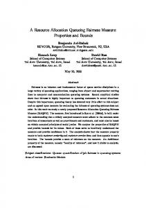
Figure 2: System Unfairness For M/M/1 Figure 2 depicts FD2 as a function of ρ for the policies studied above, under the M/M/1 queue, for µ = 1. The figure demonstrates the following properties: 1. In terms of unfairness the policies may be ranked as P-LCFS > NP-LCFS > ROS > FCFS > PS. That is, Preemptive LCFS is the most unfair and Processor sharing is the most fair. This dominance is observed for all values of ρ, except for ρ → 0. 2. At ρ → 0 the unfairness measures of all policies converge, as expected, and all policies experience full fairness, (E[D2 ] = 0). This results from the fact that most customers find an empty system upon arrival and thus are subject to no discrimination. 3. Processor sharing is the only policy (of the policies studied) whose fairness is absolute (unfairness = 0). 4. The system unfairness seems to be monotone increasing in the system utilization ρ for all policies except PS. For FCFS and ROS the increase is modest, and the values at ρ = 0.9 are relatively small. In fact the slopes of their curves suggest that when ρ → 1 their values may converge to a finite number (in contrast, for example, to the

26

expected delay, which blows up at ρ = 1). For the LCFS policies the increase is very drastic at high loads. It is interesting to compare these results with the policy ranking provided by the orderfairness proposed in Avi-Itzhak and Levy (2004) and the slow-down fairness approach used in Wierman and Harchol-Balter (2003). Recall that the former measure ranks FCFS as the most fair and LCFS as the most unfair, while the latter achieves a somewhat reverse ranking when it classifies LCFS preemptive as always fair and FCFS as unfair. Our results above demonstrate that in the M/M/1 case RAQFM concurs with the order-fairness as it ranks FCFS as the most fair (of the non-PS policies examined numerically) and LCFS as the most unfair. The reason for this behavior is that in the M/M/1 model the issue of seniority difference is dominant over the issue of service time differences for the compared disciplines.

5.2

The Tradeoff Between Seniority and Service Times and RAQFM’s Sensitivity to it

The prior example demonstrated that when the seniority differences dominate service time differences, RAQFM properly ranks the policies by their seniority preferences. Our aim in the next example is to demonstrate the sensitivity of RAQFM to service time discrepancies and show that when this factor dominates the seniority factor, RAQFM reacts properly. To this end we next consider a case where the arrivals remain Poisson while the variability of service times increases drastically. This is achieved by a bi-valued service time whose values are s = 0.1 with probability p and s0 = 10 with probability 1 − p. The value of p is selected to be p = 90/99 = 0.9009 so as to have mean service time of 1, identical to the previous numerical example. The variance of this service time is ps2 + (1 − p)s02 = 9.1, in comparison to the variance of the M/M/1 case which was 1/µ2 = 1. This system is analyzed via a simulation program, which was run on each evaluated point for at least 106 customers. Figure 3 depicts FD2 as a function of ρ for the FCFS, LCFS and P-LCFS cases.

27

35 Non−Preemptive LCFS FCFS Preemptive LCFS 30

25

FD2

20

15

10

5

0

0

0.1

0.2

0.3

0.4

ρ

0.5

0.6

0.7

0.8

0.9

Figure 3: System Unfairness For Discreet Distribution The figure demonstrates that over the range ρ = (0, 0.55) RAQFM ranks P-LCFS as the most fair among the 3 policies, in contrast to its ranking in the M/M/1 case. As such, it concurs, in this case, with the ranking of the slow-down fairness approach (Wierman and Harchol-Balter (2003)) and is in contrast with the order fairness approach (Avi-Itzhak and Levy (2004)). To understand this, note that due to the large variability of service times, large discriminations (and unfairness values) are formed when a large job is served and many small jobs queue behind it. In such cases preemption of large jobs from service can alleviate this problem. P-LCFS achieves this since it tends to preempt the large jobs with high probability. Thus, in the case of high variability service times, where service time differences dominate seniority differences, P-LCFS can be more fair than FCFS due to giving preferential treatment to short jobs over long jobs, despite its preferential service to less-senior jobs over more-senior jobs. In summary, the examples presented in Figures 2 and 3 demonstrate how RAQFM accounts for the tradeoffs between seniority differences and service times differences. It should be noted that in the second example the lower unfairness of P-LCFS does not hold for the whole range of utilizations. For high load situations P-LCFS becomes again the most unfair policy. This may possibly be attributed to the fact that at high loads the queue size tends to be large and thus the magnitude of order discrepancies may increase sharply (similarly to the waiting time variance). 28

6

Concluding Remarks

This work aimed at understanding the issue of fairness in queues and deriving a measure that can be used to quantify fairness in a variety of queueing systems. We Recognized that both seniority and service requirements must play significant role in scheduling decisions, and focused on proposing a measure, RAQFM, that accounts for both quantities. Our approach allows one to use RAQFM for measuring individual job discrimination under specific sample paths, as well as unfairness of scenarios and unfairness of systems and service policies. Further, the measure allows the use of common queueing theory techniques for evaluating the system unfairness. We examined the sensitivity of RAQFM to seniority and service requirement and showed that in special cases it reacts to these parameters in a proper and intuitive way. We showed that the PS service policy is uniquely absolutely fair. We further provided bounds on the measure (individual discrimination) that can be used as a scale of reference for the measure. Lastly, we used RAQFM to derive the system unfairness for the M/M/1 system under five fundamental service disciplines. Evaluation of special cases of the results suggest that this measure seems to agree with common intuition about fair and unfair queueing situations. Our analysis leads to a simple ranking of the service policies examined for the M/M/1 system, independent of the load situation, according to their relative fairness (as evaluated by RAQFM). The ranking, stated from most-fair to least-fair, is PS, FCFS, ROS, NPLCFS and P-LCFS. Studying of queueing fairness is in its early stage and more research is needed to further understand it. Our ongoing research deals with expanding the analysis of RAQFM to a wider variety of queueing systems and service policies. In particular in Raz, Avi-Itzhak, and Levy (2004a) we studied how queue prioritization affects fairness. Good understanding of fairness and proper quantification of it will allow researchers and practitioners to quantitatively account for fairness, in addition to the traditional measure of efficiency, in designing and evaluating queueing systems and scheduling policies. A comparison of the various measures of fairness in queues is important in order to better understand the subject as well as understand the situations at which each of the measures should be applied. Such comparison is provided in Avi-Itzhak, Levy, and Raz (2004).

29

References Avi-Itzhak, B. and Levy, H., 2004. On measuring fairness in queues. Advances in Applied Probability, 36(3):919–936. Avi-Itzhak, B., Levy, H., and Raz, D., 2004. Quantifying fairness in queueing systems: Principles and applications. Technical Report RRR-26-2004, RUTCOR, Rutgers University. URL http://rutcor.rutgers.edu/pub/rrr/reports2004/26 2004.pdf. Submitted. Bansal, N. and Harchol-Balter, M., 2001. Analysis of SRPT scheduling: investigating unfairness. In Proceedings of ACM Sigmetrics 2001 Conference on Measurement and Modeling of Computer Systems, pages 279–290. Bender, M., Chakrabarti, S., and Muthukrishnan, S., 1998. Flow and stretch metrics for scheduling continuous job streams. In Proceedings of the 9th Annual ACMSIAM Symposium on Discrete Algorithms, pages 270–279, San Francisco, CA. Bertsekas, D. and Gallager, R., 1987. Data Networks. Prentice-Hall. Bonald, T. and Prouti`ere, A., 2004. On performance bounds for balanced fairness. Performance Evaluation, 55:25–50. Coffman, Jr., E. G., Muntz, R. R., and Trotter, H., 1970. Waiting time distribution for processor-sharing systems. J. ACM, 17:123–130. Demers, A., Keshav, S., and Shenker, S., 1989. Analysis and simulation of a fair queueing algorithm. In Symposium proceedings on Communications architectures & protocols, pages 1–12, Austin, Texas, USA. Demers, A., Keshav, S., and Shenker, S., 1990. Analysis and simulation of a fair queueing algorithm. Internetworking Research and Experience, 1:3–26. Friedman, E. J. and Henderson, S. G., 2003. Fairness and efficiency in web server protocols. In Proceedings of ACM Sigmetrics 2003 Conference on Measurement and Modeling of Computer Systems, pages 229–237, San Diego, CA. Golestani, S. J., 1994. A self-clocked fair queueing scheme for broadband application. In Proc. IEEE INFOCOM, pages 636–646, Toronto, Canada. 30

Greenberg, A. G. and Madras, N., 1992. How fair is fair queueing? Journal of the ACM, 3(39):568–598. Hahne, E., 1991. Round-robin scheduling for maxmin fairness in data network. IEEE J. Select. Areas Commun., 9:1024–1039. Jaffe, J. M., 1981. Bottleneck flow control. IEEE Transactions on Communications, 29 (7):954–962. Kelly, F. P., 1997. Charging and rate control for elastic traffic. European Transactions on Telecommunications, 8:33–37. Keshav, S., 1997. An Engineering Approach to Computer Networking: ATM Networks, the Internet, and the Telephone Network. Addison Wesley Professional, Reading, MA. Kleinrock, L., 1964. Analysis of a time-shared processor. Nav. Res. Log. Quarterly, 11: 59–73. Kleinrock, L., 1967. Time-shared systems: A theoretical treatment. J. ACM, 14:242–261. Larson, R. C., 1987. Perspective on queues: Social justice and the psychology of queueing. Operations Research, 35:895–905. Mann, I., 1969. Queue culture: The waiting line as a social system. Am. J. Sociol., 75: 340–354. Mo, J. and Walrand, J., 2000.

Fair end-to-end window-based congestion control.

IEEE/ACM Trans. Netw., 8(5):556–567. Palm, C., 1953. Methods of judging the annoyance caused by congestion. Tele. (English Ed.), 2:1–20. Parekh, A. and Gallager, R. G., 1993. A generalized processor sharing approach to flow control in integrated services networks: The single node case. IEEE/ACM Trans. Networking, 1:344–357. Parekh, A. and Gallager, R. G., 1994. A generalized processor sharing approach to flow control in integrated services networks: The multiple node case. IEEE/ACM Trans. Networking, 2:137–150.

31

Rafaeli, A., Barron, G., and Haber, K., 2002. The effects of queue structure on attitudes. Journal of Service Research, 5(2):125–139. Rafaeli, A., Kedmi, E., Vashdi, D., and Barron, G., 2003. Queues and fairness: A multiple study investigation. Faculty of Industrial Engineering and Management, Technion. Haifa, Israel. Under review. URL http://iew3.technion.ac.il/Home/Users/anatr/ JAP-Fairness-Submission.pdf. Raz, D., Avi-Itzhak, B., and Levy, H., 2004a. Classes, priorities and fairness in queueing systems. Technical Report RRR-21-2004, RUTCOR, Rutgers University. URL http: //rutcor.rutgers.edu/pub/rrr/reports2004/21 2004.pdf. Submitted. Raz, D., Levy, H., and Avi-Itzhak, B., 2004b. A resource-allocation queueing fairness measure. In Proceedings of Sigmetrics 2004/Performance 2004 Joint Conference on Measurement and Modeling of Computer Systems, pages 130–141, New York, NY. Also appears in Performance Evaluation Review, 32(1):130-141. Rothkopf, M. H. and Rech, P., 1987. Perspectives on queues: Combining queues is not always beneficial. Operations Research, 35:906–909. Wang, Y. T. and Morris, R. J. T., 1985. Load sharing in distributed systems. IEEE Trans. on computers, C-34(3):204–217. Whitt, W., 1984. The amount of overtaking in a network of queues. Networks, 14(3): 411–426. Wierman, A. and Harchol-Balter, M., 2003. Classifying scheduling policies with respect to unfairness in an M/GI/1. In Proceedings of ACM Sigmetrics 2003 Conference on Measurement and Modeling of Computer Systems, pages 238 – 249, San Diego, CA. Wolff, R., 1982. Poisson arrivals see time averages. Oper. Res., 30(2):223–231. Zhou, Y. and Sethu, H., 2002. On the relationship between absolute and relative fairness bounds. IEEE Communication Letters, 6(1):37–39.

32