Rate Control Scheme for Consistent Video Quality in ... - IEEE Xplore

2166

IEEE TRANSACTIONS ON IMAGE PROCESSING, VOL. 20, NO. 8, AUGUST 2011

Rate Control Scheme for Consistent Video Quality in Scalable Video Codec Chan-Won Seo, Jong-Ki Han, Member, IEEE, and Truong Q. Nguyen, Fellow, IEEE

Abstract—Multimedia data delivered to mobile devices over wireless channels or the Internet are complicated by bandwidth fluctuation and the variety of mobile devices. Scalable video coding has been developed as an extension of H.264/AVC to solve this problem. Since scalable video codec provides various scalabilities to adapt the bitstream for the channel conditions and terminal types, scalable codec is one of the useful codecs for wired or wireless multimedia communication systems, such as IPTV and streaming services. In such scalable multimedia communication systems, video quality fluctuation degrades the visual perception significantly. It is important to efficiently use the target bits in order to maintain a consistent video quality or achieve a small distortion variation throughout the whole video sequence. The scheme proposed in this paper provides a useful function to control video quality in applications supporting scalability, whereas conventional schemes have been proposed to control video quality in the H.264 and MPEG-4 systems. The proposed algorithm decides the quantization parameter of the enhancement layer to maintain a consistent video quality throughout the entire sequence. The video quality of the enhancement layer is controlled based on a closed-form formula which utilizes the residual data and quantization error of the base layer. The simulation results show that the proposed algorithm controls the frame quality of the enhancement layer in a simple operation, where the parameter decision algorithm is applied to each frame. Index Terms—Rate control, scalable video coding (SVC), video quality control.

I. INTRODUCTION

S

CALABLE video coding (SVC) has been developed as an extension of the ITU-T Recommendation H.264|ISO/IEC 14496-10 advanced video coding [1], [2]. Three scalability directions (i.e., temporal, spatial, and quality scalability) and their combinations are provided by SVC [2]. The encoder structure depends on the type of scalability supported by the application. In general, the SVC encoder consists of multiple layers to provide combined scalabilities. To improve the performance of the SVC codec, many researchers have proposed schemes to reduce Manuscript received June 02, 2009; revised July 01, 2010; accepted February 28, 2011. Date of publication March 14, 2011; date of current version July 15, 2011. This work was supported in part by Hi Seoul Science/Humanities Fellowship from Seoul Scholarship Foundation and the MKE(The Ministry of Knowledge Economy), Korea, under the national HRD support program for convergence information technology supervised by the NIPA(National IT Industry Promotion Agency) (NIPA-2010-C6150-1001-0013). The associate editor coordinating the review of this manuscript and approving it for publication was Dr. Mary Comer. C.-W. Seo and J.-K. Han are with the Department of Information and Communication Engineering, Sejong University, Seoul 143-747, Korea (e-mail: [email protected], [email protected]). T. Q. Nguyen is with the Department of Electrical and Computer Engineering, University of California, San Diego, CA 92037 USA eE-mail: nguyent@ece. ucsd.edu). Digital Object Identifier 10.1109/TIP.2011.2126583

the redundancy in a layer and to remove the redundancy between layers [3]–[6]. On the other hand, to increase the coding speed, techniques using motion and residual information of the base layer have been proposed [7]–[9]. Besides increasing the performance and speed of video codec, the video quality of the encoded frames is one of the most important issues [10], [11]. Video quality control has been studied for various video codecs since quality fluctuation has a major negative effect on subjective video quality. It is important to efficiently use the target bits in order to maintain a consistent video quality or achieve a small distortion variation throughout the whole video sequence. To control the video quality at a constant level, various techniques have been proposed [12]–[16]. Vito et al. [12] have proposed a scheme to control the PSNR of the H.264 bitstream, where the picture qualities are constant over a group of pictures (GOP) using the relationship between the quantization parameter and PSNR. In [13], a novel two-pass encoding was proposed to achieve constant video quality with variable bit rate (VBR) for video storage applications using MPEG-2, where rate–quantization (R-Q) and distortion–quantization (D–Q) models are formulated. Two-pass VBR encoding is quite effective from the perspective of coding performance, but suffers from relatively high computational complexity. In previous researches [14], [15], constant video quality is achieved in the Motion JPEG 2000 system which uses a wavelet-based scheme. In [16], a trellis-based algorithm is applied to reduce quality variation. A lot of conventional research [16], [17] assumes that constant QP for the entire video sequence typically yields good coding performance and uniform visual quality. The constant QP schemes provide the advantages of low computational complexity and low encoding delay. However, it is a challenge to achieve a good solution for the hierarchical B picture structure of SVC, because temporal distances between the current and reference frames are not uniform in the structure. For example, in the hierarchical B picture structure with GOP size 8, temporal distances between the current and the reference frames are 1, 2, 4, and 8 at temporal levels 3, 2, 1 and 0, respectively. In this GOP structure, the amounts of residual signal vary according to the temporal distance. Thus, it is not simple to maintain a consistent quality for frames, because the frames in each temporal level could have different relationships between bit rate and quality. Quality control techniques for scalable bitstream have been proposed in [18] and [19], where the fine grain scalability (FGS) module of MPEG-4 is modified to generate constant quality data. The FGS layer encodes the transform coefficients in the form of an embedded bitstream which is truncated at any arbitrary point. In the standardization process for SVC, FGS had been discussed as one of the quality scalability schemes, and it is also an effective scheme to control

1057-7149/$26.00 © 2011 IEEE

SEO et al.: RATE CONTROL SCHEME FOR CONSISTENT VIDEO QUALITY IN SCALABLE VIDEO CODEC

quality with flexibility. Nevertheless, since the complexity of FGS modules is very high [20], [21], the FGS technique has not been adopted in the Scalable Baseline Profile, Scalable High Profile, and Scalable High Intra Profile of SVC [22]. In this paper, we consider a system supporting spatial scalability without FGS. To achieve consistent video quality of the enhancement layer throughout the video sequence, a target distortion for each frame is assigned. The distortion of the enhancement layer is derived from coding information of the base layer in the closed form formula. Based on this formula, the quantization parameter is chosen to control the video quality of the spatial enhancement layer. The proposed algorithm yields an SVC bitstream whose quality is controllable according to an arbitrary target PSNR. This paper is organized as follows. In Section II, we briefly introduce the coding modes adopted in SVC. In Section III, the problem considered in this paper is formulated, where the coding distortions generated in the base layer and enhancement layer are derived. In Section IV, we propose a control algorithm to maintain a consistent video quality or to achieve a small distortion variation throughout the whole video sequence. Simulation results are presented in Section V. Section VI concludes the paper. II. CODING MODES IN SVC In order to improve the coding efficiency of the enhancement layer in SVC codec, prediction modes using the coding information of the base layer are employed. The enhancement layer is coded using inter-layer prediction to remove redundancy between layers [1], [2]. The texture, motion, and residual information of the base layer are used as predictive data for the enhancement layer when inter-layer prediction is applied. Coding modes adopted in the SVC standard are briefly described as follows. A. Texture Prediction Mode The texture prediction mode is considered for a macroblock in the enhancement layer when the corresponding block in the base layer has been encoded with intra mode. The corresponding intra blocks reconstructed in the base layer (the lower resolution layer) are upsampled by applying a four-tap FIR interpolation filter when the resolutions of two layers are different. The difference between the upsampled signal and macroblock of the enhancement layer is encoded [2], [24] where is used to indicate macroblocks encoded by the texture prediction mode. B. Motion Prediction Mode When a block in the base layer is encoded by inter mode, the corresponding macroblock in the enhancement layer uses motion information of the block in the base layer. In this mode, the partitioning information, the reference indexes and motion vectors of a block in the enhancement layer are derived from the data of the corresponding block in the base layer. When the resolution of the enhancement layer is 4 times larger than that of the base layer, the motion vector and partitioning data of the base layer are up-scaled by a factor of 2 without motion estimation and mode decision for the enhancement layer [2]. When the

2167

TABLE I TOTAL CPU TIMES CONSUMED BY SVC ENCODER ARE MEASURED IN THE RESOLUTION OF 1=1000 SECOND ACCORDING TO THE OPTIONS FOR INTER-LAYER PREDICTION

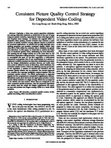
motion prediction mode is applied for the current macroblock is set to “1.” in the enhancement layer, C. Residual Prediction Mode The residual prediction mode is considered when a current block in the enhancement layer and the corresponding macroblock in the base layer are encoded by inter mode. In this mode, the residual signal of the base layer is upsampled by a block-wise bilinear filter to be used as a predictive signal for the enhancement layer [2], [3]. An additional flag, , is encoded and transmitted to indicate that the current macroblock is encoded with residual prediction mode. In this mode, the difference signal between the residual data of the two layers is encoded. III. PROBLEM FORMULATION The SVC encoder can choose one of three options related to the inter-layer prediction; 1) no; 2) yes; or 3) adaptive. Option “no” means inter-layer prediction is not used, where the base and the enhancement layers are independently encoded using motion estimation. When option “yes” is selected, prediction modes described in Section II are always used without motionestimation in the enhancement layer. In the “adaptive” option, after the enhancement layer is encoded using both temporal motion estimation and inter-layer prediction, one of the temporal and inter-layer predictions is selected for each macroblock. The coding performance and computational complexity of the SVC codec depend on the option for inter-layer prediction. Since the encoding using the “adaptive” option has to do both prediction schemes, the “adaptive” option requires much more complexity than the other options. The CPU times consumed by the SVC encoder are compared according to the options for inter-layer prediction in Table I, where “FOOTBALL,” “FOREMAN,” “TEMPETE,” and “SOCCER” are used as test sequences. One hundred frames are encoded for each sequence, the size of GOP is set to 8, and resolutions of the base and enhancement layers are set to QCIF and CIF, respectively. As observed from this table, the codec using “2) yes” is much simpler than that for “1) no” and “3) adaptive.” To check how the coding performance is affected by the coding option, we compare the RD curves of SVC codecs using the various options in Fig. 1. Although the codec using “3) adaptive” shows better performances than others, it has very high complexity. In this paper, we consider a real time application with low coding delay. Since the inter-layer prediction mode can increase the coding efficiency of the SVC encoder with low complexity, we consider a SVC system whose

2168


current frame are the sum of the motion-compensated frame and the quantized residual signal

(4) where denotes the reconstructed residual signal corrupted from the quantization error. Substituting (3) and (4) into (2) yields (5) The distortion of the base layer coded by H.264 encoder is represented as Fig. 1. RD curves according to the options for inter-layer prediction. GOP size and are f38 33 28 23g and f42 37 32 27g, respectively. is 8.

QP s

QP s

; ; ;

; ; ;

inter-layer prediction option is set to “2) yes,” where the motion of the enhancement layer is the upscaled version vector of the base layer, and where texture and of motion vector residual predictions of the base layer are reused. An encoder structure for the SVC reference software (JSVM) [24] using the inter-layer prediction mode is represented in Fig. 2, where the bitstream compressed in the spatial base layer is compatible with H.264/AVC [2], [25]. The data of the enhancement layer are encoded by coding the difference between the residual data of the enhancement layer and the base layer. Since the spatial resolution of the base layer is different to that of the enhancement layer, the residual data of the base layer have to be up-sampled to the resolution of the enhancement layer when the inter-layer prediction mode is used.

(6) where subscript denotes the base layer. The residual data denotes the difference between the original and motioncompensated data in the base layer (7) where is the signal compensated by motion vector of the base layer. B. Distortion of the Enhancement Layer

and are the width and the height of a frame, respecwhere and are the th pixel value in the original tively, and and the reconstructed frames, respectively. The original signal of the current frame can be represented as the sum of the motion-compensated signal and the residual signal generated from the motion estimation (ME) process as follows:

In Fig. 2, the current original frames of the enhancement and and , respectively, the base layers are denoted by where subscript denotes enhancement layer. The letters and denote the indexes of pixel positions in frames of the base and and the enhancement layers, respectively, where . Since the resolution of the enhancement layer is times larger than that of the base layer, the number of total pixels in the enhancement frame is , where is set to 4 as an example in this paper. Similarly, the motion-compensated and , which are recondata are represented by structed from the original motion-compensated frames and ; they include quantization errors, and , and . i.e., Since the inter-layer prediction option is set to “yes,” the differand ) resulting ence between the prediction error ( from the ME process in the base and enhancement layers is enand the residual data coded, where of base layer have to be upscaled to the resolution of the enhancement layer. The data to be encoded in enhancement , shown as follows, which is the layer are denoted by difference between the prediction error of the enhancement layer and the upscaled version of the prediction error of , as shown in Fig. 2: the base layer,

(3)

(8)

denotes the motion-compensated frame using the rewhere constructed reference frames. The residual signal resulting . The reconstructed data of the from ME is

implies the residual upscaling process with where two taps used in JSVM [2], [24]. For a particular , the upscaled signal is made by filtering and

A. Distortion of the Base Layer PSNR depends on the coding distortion as follows: PSNR

(1)

In (1), represents the mean squared difference between the original and the reconstructed frames and is given by (2)


2169

Fig. 2. SVC encoder structure using inter-layer prediction.

with a two–tap coefficients defined in JSVM [2], [24], and . where The quantization error of the current frame in the base layer is

is a quantization process for the enhancement where layer. Applying (5) to the enhancement layer gives the mean squared distortion of the enhancement layer as follows:

(9)

Substituting (4) and (3) into yields

and

(14)

, respectively,

(10) Thus

where and are represented in (12) and (13), respectively, which imply the original and the reconstructed data in the enhancement layer of Fig. 2. C. Relationship Between Two Layers

(11)

Substituting (11) into (8) gives

The relationship between data for the enhancement and base layers can be represented as

(15) (16) (12)

The reconstructed data for

are

(13)

where implies the up-sampling process using a bilinear filter with two taps [26]. Note that and are linear functions, where is used for a frame level whereas is applied for a block level. and denote scaling errors generated from up-scaling the base layer data into the resolution of the enhancement layer data.

2170


The relation between (15) and (16) as follows:

and

is represented by using

when a target PSNR which provides the corresponding is assigned. In the proposed scheme, a quantization parameter is decided to result in . In (19), we can see that depends on the residual of the base , the upsampling errors , , and the quanlayer , , and . Among these values, tization errors , , and are known when the enhancement layer is encoded, since the base layer has been encoded before the is also known since the motion-comenhancement layer. has been encoded when the current frame pensated frame is encoded in the enhancement layer. can be calculated simply by upscaling into the resolution of the enhancement layer, as follows: (21)

(17) in (12) is represented by using (17) as follows:

(18) Substituting (18) into (14) gives

is already encoded Since the motion-compensated frame is encoded, is set to the value when the current frame was encoded. Thus, all values which was calculated when in the parentheses of (19) are known or easily calculated before is controlled by applying the enhancement layer is encoded. to the known values. the quantization function The SVC encoder employs a scalar quantizer, where 52 quantization steps are used. These values are indexed by the [25]. In (19), the quantized value quantization parameter has to be calculated with 52 ’s. In the producing is selected among 52 proposed scheme, a ’s. The proposed algorithm to control the video quality is summarized in Table II. In Table II, when Intra frame is encoded, , , and in (19) are set to 0 for all and because the motion-compensated frame is not used. Since the frame of the base layer is encoded with Intra mode, and are used instead of and , respectively, where is an upsampling process applied to the intra data defined in JSVM and used for Intra frame are [27]. Therefore, defined as

(19) which describes the relationship between the distortion of the enhancement layer and the data resulting from encoding the is base layer and motion-compensated frame. In Section IV, evaluated by applying the function into the previously engives a quantization parameter gencoded data. Evaluating erating the target quality of enhancement layer.

(22)

IV. CONTROL SCHEME FOR CONSISTENT VIDEO QUALITY A. Control Algorithms

(23)

Here, we discuss control algorithms used to maintain a consistent video quality throughout the entire sequence. PSNR of the enhancement layer is controlled by adjusting the quantizaof the enhancement layer. Equation (1) is tion parameter rewritten for the enhancement layer as follows: PSNR

(20)

and In Table II, when an Intra frame is encoded, are obtained from encoding the base layer. In Step 2, is is calculated using a linear upcalculated by (21). sampler. is calculated by the intra upis calculated by (22) in scaling filter used in JSVM. ’s are calculated for all posStep 3. In Step 4, sible ’s. producing the PSNR which is the closest to


PROPOSED

QP

TABLE II DECISION ALGORITHM TO CONTROL PSNR FOR A FRAME

2171

TABLE IV DECISION ALGORITHMS FOR , THE NUMBER OF QUALITY ENHANCEMENT FOR EACH FRAME LAYERS IN FGS, AND BIT PLANES TO CONTROL

QP

PSNR

TABLE V FIXED QP ALGORITHM TO CONTROL THE AVERAGED PSNR OF A SEQUENCE

BRUTE FORCE

QP

TABLE III DECISION ALGORITHM TO CONTROL PSNR FOR EACH FRAME

PSNR is selected in Step 5. After encoding the enhancement layer with the selected , and are saved into and to be used as the temporary buffer and in encoding the next non-Intra frame. In Table II, when a non-Intra frame is encoded, , , are obtained from encoding the base layer. In Step 2, and is calculated from (21). and are calculated by using a linear upsampler. and are obtained by reading the data indicated by from and . is found the using residual up-scaling filter used in JSVM. The signal is calculated by (18) in Step 3. To compare the proposed approach with other conventional approaches, we considered some techniques proposed in [12]–[17]. However, since [12], [16], [17] had been proposed to control the video quality in “IPPP” structure only, they cannot provide consistent video quality in hierarchical B picture structure. The reason is that the temporal distances between the current and reference frames in hierarchical structure are not uniform. Other schemes [13]–[15] cannot properly be applied to SVC, since they had been proposed for MPEG-2

and JPEG2000. In this paper, we consider the brute force, FGS and the fixed QP algorithms as conventional schemes, which are summarized in Tables III–V, respectively. The brute force algorithm uses a multiple encoding method for a frame. In Step 1 of Table III, the enhancement layer is encoded repeatedly with ’s. The generating a PSNR which is the closest 52 to the target PSNR is selected in Step 2. The quality control algorithm using FGS is described in Table IV. In Step 2, is selected to generate a PSNR which is lower than the target PSNR and the closest to the target PSNR . Then, all of the quality enhancement layers are encoded in Step 4, where each layer consists of multiple bit planes. In Step 5, the number of quality enhancement layers and bit planes generating a PSNR which is the closest to the target PSNR is selected. In Table V, the fixed QP algorithm encodes a sequence with all possible values. In Step 1, the base and enhancement layers of a and . Step 1 is sequence are encoded with a fixed repeated for 52 ’s. Since storing the entire encoded data set for the base layer of a sequence is impossible, the base layer even if it increases is also encoded repeatedly with a fixed generating an average encoding complexity. In Step 3, the which is the closest to target is selected. B. Comparison of Algorithm Complexity Let us denote the complexities of the encoding procedures and for the base layer and the enhancement layer by , respectively. includes complexities of modules required to encode the base layer by the H.264 encoder. denotes the complexity required to encode the en. In Step 2 of Table II, hancement layer with a operations are required to calculate , , and for a fixed , respectively. represents

2172


the complexity of operations used in linear filtering to interpolate the base layer signal. The complexities associand are almost negligible, ated with obtaining since they have been already calculated when the previous frame was encoded. The complexities required to calculate for a fixed are denoted by , which is the complexity of the upscaling module for the residual signal. In Step 3, a summation of seven terms is required to for a fixed , where the complexity is calculate . In Step 4, is required to evaluate denoted by for a fixed . In Step the quantized signals 5, we can simply choose a among 52 ’s, where is required. The overall computational complexity of the proposed algorithm is described as proposed

(24) Overall complexity of the brute force scheme shown in Table III is brute force (25) Overall complexity of the FGS scheme shown in Table IV is FGS (26) where denotes the averaged computational complexity to encode a group of bit planes. In the FGS scheme, the number of bit planes to be encoded at each step can be set to an arbitrary number. denotes the number of total steps required to encode all bit planes in the FGS layer. In this paper, is set to 60 which means a FGS layer consists of 20 groups of bit planes since the total number of FGS layers is 3. The overall complexity of the fixed QP scheme shown in Table V is fixed (27) which is the overall complexity for the entire sequence. In (24)–(27), complexities of modules are variable according to the coding conditions such as sequence, bit rate, inter layer coding relationships, and so on. From simulation results with various test sequences, we compute the relative values of those as follows, where “FOREMAN,” “FOOTBALL,” and “BUS” is set to 352 288. GOP are used as test sequences, and size is set to 8.

Fig. 3. The P SNR of enhancement layer is controlled by various algorithms. GOP size is 16. Target P SNR dB. (a) QP , (b) QP .

= 40

= 35

= 36

As we can see from these values, the and the are much larger than the other values except for . Based on (24)–(27), it is estimated that the proposed scheme can reduce encoding complexity by about 79%, 90%, and 93% compared with the brute force, FGS and fixed QP schemes, , , respectively. In this estimation, complexities of and are not considered since the values are negligible. Therefore, we conclude that the proposed scheme is much simpler than the conventional schemes. V. SIMULATION RESULTS Here, we show the simulation results to evaluate the performance of the proposed algorithm. We apply the proposed algorithm to the SVC reference software, JSVM 9.14 [24], where the option for inter-layer prediction is set to “yes,” and the resoand lutions of the two layers are , respectively. In the simulations, only the luma component is considered since the luma component is much more significant than the chrominances in the measurement of video quality. However, the proposed scheme can be applied easily to all color components.


AVERAGED

AVERAGED

D

D

AND

TABLE VI CI WHICH DENOTES 95% CONFIDENCE INTERVAL OF PSNR PSNR VALUES. PSNR dB dB dB dB . THE SIZE OF GOP IS 16

= f32 ; 36 ; 40 ; 44 g

TABLE VII TYPE. TEST SEQUENCE IS “BUS.” GOP SIZE IS 16

FOR FRAME

QP

IS

40.

TABLE VIII AVERAGED SSIM FOR QP DECISION ALGORITHMS. . TARGET PSNR dB dB dB dB . THE SIZE OF GOP IS 16

QP = f42; 38; 34; 30g = f32 ; 36 ; 40 ; 44 g

Fig. 3 shows PSNRs of the sequence “FOOTBALL” when the target PSNR of the enhancement layer is set to 36 dB. It is well known that fixed QP scheme achieves consistent quality throughout the entire sequence with IPPP structure if video sequences are stationary [12]. However, since I, P and B frames are used in hierarchical structure of SVC, the fixed QP scheme is not suitable for SVC as shown in Fig. 3. The performances of various schemes are summarized in Table VI, where the averaged difference value between the target and actual PSNRs PSNR PSNR ) are summarized for (i.e., various test sequences. The averaged values of the brute force and the proposed schemes are about 0.18 dB and 0.24 dB, respectively. 95% confidence intervals (CI) are also calculated in Table VI. The CI value of the proposed scheme is as very small as that of the brute force scheme. Simulation results obtained when the target PSNR ’s are set according to frame types (I, P, B) are shown in Table VII. These results indicate that the proposed scheme can control the video quality effectively with simple operations under various test conditions. Although the accuracy of the FGS scheme is the best, the computational complexity of the FGS is extremely high as much as that of the fixed QP scheme described in the previous section. The brute force

0

2173

QP = f42; 38; 34; 30g. TARGET

scheme also can control PSNR precisely without FGS layers, though the scheme is quite complex. We can see from these results that the performance of the proposed scheme is similar to that of the brute force scheme while the proposed scheme is much simpler than the brute force scheme. To analyze the performances of the schemes in terms of perceptual quality, Structural SIMilarity (SSIM) [28] is used as a quality metric in Table VIII. The averaged SSIM values of all schemes are high and are very similar to each other. These results mean that the perceptual qualities of sequences encoded by all schemes are acceptable and properly controlled. In order to check the performances with respect to RD optimization, the averaged PSNRs of the encoded images ’s are evaluated at different bit rates in Fig. 4, where and the target PSNR ’s are set are set to dB dB dB dB . The proposed scheme has to very similar RD performance to the other schemes. JSVM has the best RD performance among the tested schemes, because the JSVM encoder assigns bits to each frame to improve RD to maintain performance whereas other schemes control consistent video quality. On the other hand, bit rate fluctuations of the schemes are shown in Table IX and indicate that the encoders using quality control schemes perform better than JSVM in systems transmitting video sequences. We conclude from these results that the proposed scheme does not result in significant degradation with respect to RD optimization while it produces consistent video quality over the entire sequence with small variation of bit rate. is assigned prior As we can see from Step 0 in Table II, to encoding the enhancement layer. From the point of view of controlling the quality of the enhancement layer, the selection does not affect the performance, as shown in Fig. 3 and of Tables VI–VIII. On the other hand, in terms of RD optimizamay affect the performance as shown tion, the selection of ' are used. As shown in in Fig. 5, where is set to a small number (e.g., 16), RD perFig. 5, when formance is poor around the low bit rate region. In this case, small bits are assigned to the enhancement layer whereas high bit rate is allocated to the base layer. Due to this setting, there is large difference between the qualities of temporal reference frames of the base and enhancement layers. This difference reduces the similarity between residual signals of both layers and consequently coding performance decreases with respect to RD is large (e.g., optimization. On the other hand, when the 32), the R-D performance decreases because the base layer is

2174


Fig. 5. RD curves resulting from SVC codec using the proposed scheme. f g. Target PSNR f dB dB dB dBg.

QP = 32;28;16

= 32 ; 36 ; 40 ; 44

force scheme, fixed QP scheme and FGS scheme, respectively. In Table X, the consumed CPU time reduction ratio is evaluated by time(proposed scheme) time(conventional scheme)

QP =

Fig. 4. RD curves resulted from SVC codecs using various algorithms. f dB dB dB dBg. (a) The f g. Target Size of GOP is 8., (b) The Size of GOP is 16.

42; 38;34;30

PSNR = 32 ; 36 ; 40 ; 44

TABLE IX VARIATION OF GENERATED BITS PER FRAME. THE SIZE OF GOP IS 16. TARGET PSNR dB.

= 40

QP = 32

encoded with insufficient information to be useful for the enhas hancement layer. This figure implies that the smaller to be used for the higher PSNR , although the selection of does not affect the ability to control PSNR . To check the complexity of the proposed algorithm, the CPU times consumed by the SVC encoders are compared in Table X, where the simulations were carried out with a Pentium-4 personal computer. We checked the elapsed CPU time at a resolusecond. Each simulation is performed 50 times tion of to obtain the averaged CPU times whose 95% CI’s are 920, 7251, 8297, and 11828 msec with the proposed scheme, brute

(28)

where conventional scheme means the brute force or FGS or fixed QP schemes. The time(proposed scheme) and time(conventional scheme) represent the CPU times consumed to encode both the base and the enhancement layers by the proposed and conventional schemes, respectively. As observed from the results, the proposed scheme requires much smaller computing time than the brute force, FGS and fixed QP schemes. This is due to the fact that the proposed scheme can with simple operations, whereas the brute force decide a and FGS schemes have to encode the frames of the enhancement layer repeatedly. These results imply that the proposed algorithm exhibits significant improvement in the reduction of computational complexity comparing with the brute force, FGS and the fixed QP schemes, while maintaining similar image quality. The proposed scheme can be useful with IPPP structure. To check the performances for IPPP structure, a scheme described in [12], some conventional schemes and the proposed scheme are compared in Fig. 6. In this simulation, we add a scheme that modified from the proposed (MP) scheme. Since there is a linear relationship between QP’s and PSNR’s of I and P frames [29], the MP scheme uses operations described in Table XI in’s are stead of Steps 4 and 5 in Table II. In Fig. 6(a), about 0.05 dB, 0.20 dB, 0.23 dB, 0.34 dB, 0.56 dB and 0.63 dB for the FGS scheme, the brute force scheme, the proposed scheme, the MP scheme, a conventional scheme [12] and the fixed QP scheme, respectively. In Fig. 6(b), averaged encoding of [12] is about 2 and 1.5 times times are shown. The larger than those of the proposed scheme and MP scheme, respectively, while the encoding time of the MP scheme is very similar to that of [12]. From these results, we conclude that the


AVERAGED CPU TIME

=

[1 1000

2175

TABLE X s] CONSUMED BY SVC ENCODERS USING QP DECISION ALGORITHMS. = f32 dB 36 dB 40 dB 44 dBg. THE SIZE OF GOP IS 16

PSNR

;

;

;

QP

QP

=

f42; 38; 34; 30g. TARGET

; ; ;

Fig. 6. Accuracy and encoding complexity resulted from SVC codecs using various algorithms for IPPP structure. = f40 36 32 , (b) The CPU time consumed by encoding the base and enhancement layers.

f32 dB; 36 dB; 40 dB; 44 dBg. (a) The averaged D

TABLE XI STEPS 4 AND 5 IN MP SCHEME

28

g. Target PSNR

=

Several simulations conclude that the proposed method yields similar video quality to that using the brute force method but reduces the complexity significantly. REFERENCES

proposed scheme and MP scheme are also effective for IPPP structure. VI. CONCLUSION We have proposed an efficient algorithm to maintain a consistent video quality throughout the entire sequence in SVC. The proposed scheme consists of encoding the base layer, the quantization parameter decision and encoding the enhancement layer with the selected parameter. Since the proposed scheme can calculate PSNR efficiently based on the closed-form formula, the video quality can also be controlled efficiently.

[1] Advanced Video Coding for Generic Audiovisual Services, , Jan. 13, 2009, ITU-T Rec. H.264 and ISO/IEC 14496-10(MPEG-4 AVC). [2] H. Schwarz, D. Marpe, and T. Wiegand, “Overview of the scalable video coding extension of the H.264/AVC standard,” IEEE Trans. Circuits Syst. Video Technol., vol. 17, no. 9, pp. 1103–1120, Sep. 2007. [3] H. Schwarz, T. Hinz, D. Marpe, and T. Wiegand, “Constrained interlayer prediction for single-loop decoding in spatial scalability,” in Proc. IEEE Conf. Image Process., Sep. 2005, vol. 2, pp. 870–873. [4] W.-J. Han, “Modified IntraBL Design Using Smoothed Reference,” Bangkok, Thailand, 2006, Joint Video Team of ISO/IEC MPEG and ITU-T VCEG, JVT-R091. [5] I. H. Shin and H. W. Park, “Adaptive up-sampling method using DCT for spatial scalability of scalable video coding,” IEEE Trans. Circuits Syst. Video Technol., vol. 19, no. 2, pp. 206–214, Feb. 2009. [6] R. Zhang and M. L. Comer, “Efficient inter-layer motion compensation for spatially scalable video coding,” IEEE Trans. Circuits Syst. Video Technol., vol. 18, no. 10, pp. 1325–1334, Oct. 2008. [7] H. Li and C. Wen, “Fast mode decision for spatial scalable video coding,” in Proc. IEEE Int. Symp. Circuits Syst., May 21–24, 2006, pp. 3005–3008. [8] H. Li, Z. G. Li, and C. Wen, “Fast mode decision algorithm for interframe coding in fully scalable video coding,” IEEE Trans. Circuits Syst. Video Technol., vol. 16, no. 7, pp. 889–895, Jul. 2006. [9] C. S. Park, S. J. Baek, M. S. Yoon, H. K. Kim, and S. J. Kim, “Selective inter-layer residual prediction for SVC-based video streaming,” IEEE Trans. Consum. Electron., vol. 55, no. 2, pp. 235–239, Feb. 2009.

2176

[10] C. S. Kim, S. H. Jin, D. J. Seo, and Y. M. Ro, “Measuring video quality on full scalability of H.264/AVC scalable video coding,” IEICE Trans. Commun., vol. E91-B, no. 5, pp. 1269–1278, May 2008. [11] G. Zhai, J. Cai, W. Lin, X. Yang, and W. Zhang, “Three dimensional scalable video adaptation via user-end perceptual quality assessment,” IEEE Trans. Circuits Syst. Video Technol., vol. 54, no. 9, pp. 719–727, Sep. 2008. [12] F. D. Vito and J. C. De Martin, “PSNR control for GOP-level constant quality in H.264 video coding,” in Proc. IEEE Int. Symp. Signal Process. Inf. Technol., Dec. 2005, pp. 612–617. [13] K. Wang and J. W. Woods, “MPEG motion picture coding with long-term constraint on distortion variation,” IEEE Trans. Circuits Syst. Video Technol., vol. 18, no. 3, pp. 294–304, Mar. 2008. [14] K. Wang and J. W. Woods, “Resource-constrained rate control for motion JPEG2000,” IEEE Trans. Image Process., vol. 12, no. 12, pp. 1522–1529, Dec. 2003. [15] Z. Ni and J. Cai, “Constant quality aimed bit allocation for 3-D wavelet based video coding,” in Proc. IEEE Int. Conf. Multimedia and Expo, Jul. 2006, pp. 121–130. [16] K. L. Huang and H. M. Hang, “Consistent picture quality control strategy for dependent video coding,” IEEE Trans. Image Process., vol. 18, no. 5, pp. 1004–1014, May 2009. [17] B. Xie and W. Zeng, “A sequence-based rate control framework for consistent quality real-time video,” IEEE Trans. Circuits Syst. Video Technol., vol. 16, no. 1, pp. 56–71, Mar. 2006. [18] X. M. Zhang, A. Veltro, Y. Q. Shi, and H. Sun, “Constant quality constrained rate allocation for FGS-coded video,” IEEE Trans. Circuits Syst. Video Technol., vol. 13, no. 2, pp. 121–130, Feb. 2003. [19] J. Sun, W. Gao, and Q. Huang, “A novel FGS base-layer encoding model and weight-based rate adaptation for constant-quality streaming,” in Proc. 3rd Int. Conf. Image Graphics, Dec. 2004, pp. 373–376. [20] J. Ridge, X. Wang, I. Amonou, and N. Cammas, “Simplification and Unification of FGS,” Geneva, Switzerland, 2006, Joint Video Team of ISO/IEC MPEG and ITU-T VCEG, JVT-S077. [21] I. Amonou and N. Cammas, “Complexity Reducion of FGS Passes,” Bangkok, Thailand, 2006, Joint Video Team of ISO/IEC MPEG and ITU-T VCEG, JVT-R069. [22] T. Wiegand, G. Sullivan, J. Reichel, H. Schwarz, and M. Wien, “Study Text (Version 3) of ISO/IEC 14496-10: 2005/FPDAM3 Scalable Video Coding,” San Jose, CA, 2007, Joint Video Team of ISO/IEC and ITU-T VCEG, N8962. [23] J. Reichel, H. Schwarz, and M. Wien, “Joint Draft 7 of SVC Amendment,” Klagenfurt, Austria, 2006, Joint Video Team of ISO/IEC MPEG and ITU-T VCEG N8242. [24] J. Vieron, M. Wien, and H. Schwarz, “Draft Reference Software for SVC,” Hannover, Germany, 2008, Joint Video Team of ISO/IEC MPEG and ITU-T VCEG, JVT-AB203. [25] T. Wiegand, G. J. Sullivan, G. Bintegaard, and Luthra, “Overview of the H.264/AVC video coding standard,” IEEE Trans. Circuits Syst. Video Technol., vol. 13, no. 7, pp. 560–576, Jul. 2003. [26] J. Astola and L. Yaroslavsky, Advances in Signal Transforms: Theory and Applications. New York: Hindawi, 2007. [27] A. Segall and J. Zhao, “Evaluation of Texture Upsampling With 4-Tap Cubic-Spline Filter,” China, 2006, Joint Video Team of ISO/IEC MPEG and ITU-T VCEG, JVT-U042. [28] Z. Wang, A. C. Bovik, H. R. Sheikh, and E. P. Simoncelli, “Image quality assessment: From error visibility to structural similarity,” IEEE Trans. Image Process., vol. 13, no. 4, pp. 600–612, 2004.


[29] S. C. Lim, H. R. Na, and Y. L. Lee, “Rate control based on linear regression for H.264/MPEG-4 AVC,” Signal Process.: Image Commun., vol. 22, no. 1, pp. 39–58, Jan. 2007. Chan-Won Seo was born in Incheon, Korea, on March 23, 1982. He received the B.S. and M.S. degrees from Sejong University, Seoul, Korea, in 2007 and 2009, respectively, where he is currently working toward the Ph.D. degree. His research interests include video coding, scalable video coding, and high-efficiency video coding.

Jong-Ki Han (M’09) was born in Seoul, Korea, in September 1968. He received the B.S., M.S., and Ph.D. degrees in electrical engineering from Korea Advanced Institute of Science and Technology (KAIST), Taejon, Korea, in 1992, 1994, and 1999, respectively. From 1999 to 2001, he was a Member of Technical Staff with the Corporate R & D Center, Samsung Electronics Company, Suwon, South Korea. He is currently an Associate Professor with the Department of Information and Communications Engineering, Sejong University, Seoul, Korea. His research interests include image and audio signal compression, transcoding, and VLSI signal processing.

Truong Q. Nguyen (F’05) received the B.S., M.S., and Ph.D. degree in electrical engineering from the California Institute of Technology, Pasadena, in 1985, 1986, and 1989, respectively. He is currently a Professor with the Electrical and Computer Engineering Department, University of California, San Diego. His research interests are video processing algorithms and their efficient implementation. He is the coauthor (with Prof. G. Strang) of a popular textbook, Wavelets & Filter Banks (Wellesley-Cambridge, 1997), and the author of several MATLAB-based toolboxes on image compression, electrocardiogram compression and filter bank design. He has authored or coauthored over 300 publications. Prof. Nguyen was the recipient of the IEEE TRANSACTION IN SIGNAL PROCESSING Paper Award (Image and Multidimensional Processing area) for the paper he cowrote with Prof. P. P. Vaidyanathan on linear-phase perfect-reconstruction filter banks (1992). He received the National Science Foundation Career Award in 1995 and is currently the Series Editor (Digital Signal Processing) for Academic Press. He served as an associate editor for the IEEE TRANSACTIONS ON SIGNAL PROCESSING from 1994 to 1996, IEEE SIGNAL PROCESSING LETTERS from 2001 to 2003, the IEEE TRANSACTIONS ON CIRCUITS AND SYSTEMS II—ANALOG AND DIGITAL SIGNAL PROCESSING from 1996 to 1997 and from 2001 to 2004, and for the IEEE TRANSACTIONS ON IMAGE PROCESSING from 2004 to 2005.