Abstractâ Even with the use of variable transformations, quantum-well (QW)-laser models based on the standard rate equations and a linear gain-saturation ...
JOURNAL OF LIGHTWAVE TECHNOLOGY, VOL. 15, NO. 4, APRIL 1997
717
Rate-Equation-Based Laser Models with a Single Solution Regime Pablo V. Mena, Student Member, IEEE, Sung-Mo (Steve) Kang, Fellow, IEEE, and Thomas A. DeTemple, Senior Member, IEEE
Abstract— Even with the use of variable transformations, quantum-well (QW)-laser models based on the standard rate equations and a linear gain-saturation term can possess multiple dc solution regimes for nonnegative values of injection current. In this paper, we demonstrate analytically that rate-equationbased models that employ more realistic gain-saturation terms can be transformed so that they do indeed possess a unique solution regime. We also present circuit-level implementations of these models suitable for use in SPICE. Index Terms—Circuit simulation, equivalent circuits, gain saturation, quantum-well lasers, rate equations, semiconductor lasers, SPICE.
I. INTRODUCTION
A
N important feature of rate-equation-based QW-laser models lies in their dc characteristics. A model often possesses multiple dc solution regimes, but only one of them is correct. The standard rate equations that use a linear gainsaturation term of the form ( ), where is photon density, possess three dc solution regimes. Javro and Kang [1] have reported that in most realistic applications the incorrect solution regimes can be eliminated by applying variable transformations to the rate equations. Specifically, nonphysical negative-power and high-power solutions are avoided when simulating the rate equations with a nonnegative injection current. This approach is particularly useful when dealing with circuit-level models, since without the transformations the user would have to coax the circuit simulation into the correct solution regime by specifying initial conditions and other simulation parameters [1]. Unfortunately, as we will show here, the transformations proposed in [1] do not always remove the incorrect solution regimes from the standard rate equations. While new variable transformations do work under certain conditions, the equations still present difficulties that cannot be eliminated. In fact, for certain extreme cases, they possess unrealistic solution characteristics. The problem is mostly due to the use of the linear gain-saturation term. As is immediately clear from this expression, when the photon density exceeds , this term becomes negative. It is reasonable, then, to assume that rate Manuscript received October 7, 1996; revised December 26, 1996. This work was supported by the National Science Foundation Engineering Research Center (ECD89-43166), the DARPA Center for Optoelectronic Science and Technology (MA972-94-1-0004), and an NSF Graduate Fellowship. The authors are with the University of Illinois at Urbana-Champaign, Department of Electrical and Computer Engineering, Beckman Institute for Advanced Science and Technology, Urbana, IL 61801 USA. Publisher Item Identifier S 0733-8724(97)02703-5.
equations using this term are really only useful for photon densities below this value. On the other hand, the more general , originally suggested by Channin expression of [2], is valid for any value of . In fact, the linear expression is essentially a first-order Taylor-series expansion is small. In [3], Agrawal of this saturation term when suggested another expression of the form which is also valid for . As we will show, either of these two nonlinear gain-saturation terms is suitable for obtaining models with a unique solution regime. In this paper, we identify rate-equation-based QW-laser models that possess a single solution regime for any nonnegative injection current. The first model is the standard rate equations that use the gain-saturation term proposed by either Channin or Agrawal. The second model is the rate equations along with a third equation for carriers in the laser’s separateconfinement-heterostructure (SCH) layer. In both cases, we show analytically that the transformations suggested in [1] produce models with a unique solution regime. We also describe circuit-level implementations of the models that can be readily implemented in SPICE. II. LIMITATIONS OF RATE EQUATIONS THAT USE A LINEAR GAIN-SATURATION TERM The rate equations discussed in [1] can be found in similar forms throughout the literature [4]–[7]. They are shown below (1) (2) (3) is the active region’s carrier In the above equations, density, is the photon density defined later, is the laser output power, is the injection current, is the active region volume, is the gain coefficient, is the optical transparency density, is the phenomenological gain compression factor, is the carrier lifetime, is the equilibrium carrier density, is the optical confinement factor, is the spontaneous emission coupling factor, is the photon lifetime, is the differential quantum efficiency per facet, is the emission wavelength, is the electron charge, is Planck’s constant, and is the speed of light in a vacuum. The photon density is defined as , where is the total
0733–8724/97$10.00 1997 IEEE
718
JOURNAL OF LIGHTWAVE TECHNOLOGY, VOL. 15, NO. 4, APRIL 1997
TABLE I PARAMETERS USED FOR PLOTTING THE dc SOLUTION CURVES OF THE STANDARD RATE EQUATIONS FROM [1]. THE PARAMETERS ARE FROM JAVRO AND KANG [1] AND TAKEN ORIGINALLY FROM DA SILVA et al. [5]
number of photons in the active volume and accounts for the fact that only photons in the active region are affected by gain or loss [8]. Under dc conditions, (1)–(3) have up to three solution regimes for a single value of injection current . In addition to the correct nonnegative solution regime, in which the solutions for and are nonnegative when , there are also a negative-power and a high-power regime. In order to eliminate these nonphysical solutions, the following pair of transformations was introduced in [1] for and :
(4) (5)
where is the voltage across the laser, is a diode ideality factor (typically set equal to two), is a new variable for parameterizing , is a small constant, is Boltzmann’s constant, and is the laser’s temperature. Equation (4) is a and . commonly used exponential relationship relating Both equations force and to be strictly nonnegative. Thus, by substituting (4) and (5) into (1)–(3), we have a new set of rate equations which have a dc solution for nonnegative injection current only if that solution yields nonnegative carrier and photon densities. Because under most conditions of interest the high-power solution regime corresponds to negative values for the carrier density, it would appear that (4) and (5) ensure that both of the nonphysical solution regimes are avoided. However, under certain conditions even the transformed rate equations cannot eliminate the high-power solution regime. By rewriting (1) and (2) under dc conditions, we obtain two functions relating carrier density to photon density . The intersection points of these two functions are the valid
solutions to the dc rate equations. The two functions are (6) (7) Using the laser parameters found in Table I [1], [5], we have graphed (6) and (7) in Fig. 1(a) for two different values of the injection current, 0.5 and 2.0 A. As we can see, for low enough injection currents, and will intersect at only one point where and . However, as the current increases, a second nonnegative solution may emerge, corresponding to the high-power solution regime. In Fig. 1(b), we plot (6) and (7) after doubling the values of , , and and setting cm . In this case, we have used currents of 30 and 100 mA. As we can see, the nonphysical high-power solution emerges at even lower values of injection current than before. Typically, the high-power solution regime should correspond to negative carrier densities. However, analysis of and shows that for currents greater than (8) the high-power solution regime actually yields positive carrier densities. Thus, a circuit-model implementation of the transformed rate equations proposed in [1] can still produce incorrect simulation results for high enough values of injection current. We performed an operating point analysis in SPICE for the circuit implementation of the transformed equations using the adjusted parameters of Fig. 1(b). Injection currents of 100 and 200 mA produced output powers of 8.16 and 16.4 mW, respectively, both of which correspond to the high-power solution regime. Inspection of Fig. 1 does suggest an alternative transformation that would completely eliminate the high-power solution
MENA et al.: RATE-EQUATION-BASED MODELS
719
(a)
(a)
(b)
(b)
Fig. 1. Plots of f1 and f2 from (6) and (7) for two different sets of model parameters. (a) Table I parameters. Dashed line: f1 for I = 0:5 A; dotted line: f1 for I = 2:0 A; solid line: f2 . (b) Modified Table I parameters. Dashed line: f1 for I = 30 mA; dotted line: f1 for I = 100 mA; solid line: f2 .
Fig. 2. Plots of f1 and f2 for extreme sets of model parameters. (a) �n < �nc using Vact = 9 10013 cm3 , 0 = 0:44, = 0:01, go = 5 1005 cm3 /s, No = 1:6 1019 cm03 , �n = 0:1 ns, �p = 10 ps, " = 3:4 10016 cm3 . Dashed line: f1 for I = 22:9 mA; solid line: f2 . (b) �n = �nc using parameters from (a) except for Vact = 4 10012 cm3 and �n = 0:239 ns. Dashed line: f1 for I = 42 mA; solid line: f2 .
regime. The plot of shows a discontinuity that separates the normal- and high-power solution curves. This discontinuity occurs at a value of where . Thus, a transformation which would limit the photon density to values below would eliminate the high-power regime for all values of injection current. One such transformation is (9) Unfortunately, while (9) can produce a set of rate equations with a single solution regime, it does so only for certain sets of model parameters. Comparison of the positive roots of the numerator and denominator of indicates three possible forms of this function. The typical case corresponds to that shown in Fig. 1. This occurs whenever (10)
2 2
2
2
2
However, two alternative forms of occur when and . Fig. 2(a) shows the first case, along with a when mA. Fig. 2(b) shows the second plot of when mA. While these cases are case, along with extreme, they do reveal intrinsic problems with (1) and (2), . As Fig. 2(a) demonstrates, not only especially when , but for can multiple nonnegative solutions exist for certain values of injection current such as the one shown in the figure, a valid nonnegative solution does not exist at all. As the discussion above suggests, the standard rate equations that use a linear gain-saturation term present two difficulties. First, under nonnegative current injection, multiple nonnegative solution regimes can occur even if the transformations suggested in [1] are implemented. Second, for certain extreme cases, no solution may exist. What is desired are rate equations that will have a single nonnegative solution for both carrier and photon densities for any nonnegative injection current. Fortunately, rate equations that use the more suitable
720
JOURNAL OF LIGHTWAVE TECHNOLOGY, VOL. 15, NO. 4, APRIL 1997
gain-saturation terms mentioned earlier satisfy this criteria.
forms are (14a)
III. STANDARD RATE-EQUATION MODEL WITH A SINGLE SOLUTION REGIME
(14b)
An alternative version of the standard one-level rate equations ensures that for a nonnegative injection current, exactly one solution exists with nonnegative carrier and photon densities. The equations treated henceforth are more generalized versions of (1) and (2) with the linear gain-saturation term replaced by the term proposed by either Channin or Agrawal. The new equations are shown below (11)
is the gain coefficient per quantum well, is where the optical transparency density, and is a factor obtained when linearizing the logarithmic gain around . Specifically, . The gain-saturation function can take on one of the following two forms: (15a) (15b)
(12) (13) Equation (11) relates the rate of change in carrier concentration to the injection current , the carrier recombination rate , and the stimulated-emission rate. In order to account for different recombination mechanisms, where , , and are the unimolecular, radiative, and Auger recombination coefficients, respectively. Equation (12) relates the rate of change in photon density to photon loss, the rate of coupled recombination into the lasing mode, and the stimulated-emission rate. Unlike the photon density defined in Section II, in this case the photon density is defined as [9], where is again the total number of photons in the active volume. Also, the coupling rate is generalized to allow coupling from any of the recombination terms, though in actual practice this coupling will typically only come from the radiative recombination. Thus, , where , , and are coupling coefficients. Finally, (13) relates the photon density to the output power . In the above equations, is the current-injection efficiency, is the number of quantum wells, is the volume of a single QW, is the optical confinement factor of one QW, is the group velocity of the lasing medium, is the photon lifetime, is the lasing wavelength, and is the output-power coupling coefficient. Note that we can convert (11)–(13) into a form analogous to that of (1)–(3), with missing from the stimulated emission term of (11) but included in the expression for , by using the definition for from Section II. Thus, both approaches are equivalent as long as the proper definition of is used. In the above equations, the stimulated-emission rate includes a carrier-dependent gain term as well as the gain saturation term . While the gain term can take on a number of forms, we will consider only two, namely a linear term such as that used in (1) and (2), or a logarithmic gain term such as that proposed in [10] and used previously in other laser models [9]. The logarithmic gain has been shown to be an excellent expression for describing the actual relationship between the material gain and the carrier density. The two
corresponding to the expressions proposed by Channin and Agrawal, respectively, with the confinement factor added to account for the revised definition of . As mentioned before, (15a) is often used instead of the linear gain-saturation term [11]–[13] and, unlike the latter, is positive for all . Equation (15b) is an alternate form of the gain-saturation term for semiconductor lasers and is also applicable for . When is much smaller than , (15a) can be approximated by the linear form, as can (15b) with the exception of a factor of 1/2 in the value for . However, because they are suitable for a wider range of photon densities and lead to models with a single solution regime, either of these two expressions are superior to the linear form. Despite the complexity of the above model equations, it is possible to show analytically that for any nonnegative injection current there can exist only one dc solution with nonnegative carrier and photon densities. After some rearrangement of (11) and (12) with , we get two nonlinear dc equations
(16)
(17) Equation (16) is obtained via multiplication of both sides of (12) by . Equation (17) is obtained by combining (11) and (12) in order to eliminate the stimulated-emission term. Both equations implicitly define functions and , respectively, which map out their nonnegative solutions. The intersection points of these two functions are the nonnegative solutions to the dc rate equations. Thus, in order to establish the existence of a unique nonnegative solution regime, we need only show that for each these two functions have exactly one nonnegative intersection point. First, consider the case . In this case, the only nonnegative solution that satisfies (17) is . When the carrier-dependent gain is linear, (16) is also satisfied by this solution. Thus, it is the unique nonnegative intersection point of the functions and when . When the gain
MENA et al.: RATE-EQUATION-BASED MODELS
721
TABLE II PARAMETERS FOR EVALUATING BOTH THE ONE- AND TWO-LEVEL QW-LASER MODELS THAT HAVE A SINGLE SOLUTION REGIME. THE PARAMETERS ARE TAKEN FROM [9] AND BASED ON DATA FROM A NUMBER OF SOURCES [13], [17]–[22]
is logarithmic, is undefined at . However, the approaches as . We solution to could include a small additive constant within the logarithm in ; however, in order to ensure that the gain is defined at either case, we can claim that the only possible solution when is . , the situation is more complicated. Because When and are not available, we analytical expressions for need to show indirectly that they have a single intersection point. In Appendix A, we show that for either of the two from (15), is differentiable and strictlyforms of . Furthermore, we increasing from the point (0, 0) for , which is only defined for values of in the show that interval , is strictly decreasing and continuous and . Clearly, and with will intersect exactly once at a nonnegative point within there exists exactly one this interval. Thus, for each to the dc rate equations when nonnegative solution
the gain-saturation terms of Channin or Agrawal are used. As an example of this fact, we have plotted in Fig. 3 the graphs of and when mA. We used the new model parameters of Table II, the logarithmic-gain term, and Channin’s gain-saturation term. The figure clearly indicates that there is exactly one intersection point. As we have shown, regardless of whether or not there are solution regimes with negative values for carrier or photon density, there is only one nonnegative solution to (16) and . Thus, it is possible to use the transformations (17) when of (4) and (5) in order to ensure that this solution regime is the only one that can be chosen during simulation. Using the approach taken in [1], we have implemented an equivalentcircuit model based on (4), (5), and (11)–(13) in SPICE. Unlike models based on the rate equations that use a linear gain-saturation term, this circuit model is applicable for all nonnegative values of injection current. It also supports a number of gain terms, including the logarithmic and linear
722
JOURNAL OF LIGHTWAVE TECHNOLOGY, VOL. 15, NO. 4, APRIL 1997
Fig. 3. Plot of f1 and f2 from the alternative one-level model when I = 10 mA. Dashed line: N = f1 (S ); solid line: N = f2 (S ).
expressions discussed above, as well as both forms of from (15). Fig. 4 shows the circuit implementation of the model. This equivalent circuit can be obtained through suitable manipulations of the one-level rate equations and the variable transformations. Substituting (4) and (5) into (11)–(13) and rearranging, we obtain
Fig. 4. Circuit-level implementation of the one-level QW-laser model with a single solution regime.
(27) (28) (29) (30)
(18)
(19) and . where After some additional rearrangement of (18) and (19) and the definition of suitable circuit elements, we obtain our final set of equations on which the circuit in Fig. 4 is based. After setting and using the fact that , the equations are (20) (21) (22) (23) (24)
These equations can be mapped directly into the circuit of Fig. 4 through a SPICE subcircuit that uses nonlinear dependent sources, with the general forms for the gain and gain-saturation terms replaced in actual practice by expressions from (14) and (15). Diodes and and current sources and model the linear recombination and charge storage in the device, while and model the effects of additional recombination mechanisms and stimulated emission, respectively, on the carrier density. and help model the time-variation of the photon density under the effects of spontaneous and stimulated emission, which are accounted for by and , respectively. Finally, produces the optical output power of the laser in the form of a voltage. Because the model is implemented as a subcircuit and not embedded within SPICE itself, it lends itself well to implementation by the average user. At the bottom of the next page we give an example of a SPICE input deck that implements such a subcircuit using the logarithmic gain term and Channin’s gain-saturation term. In addition to the parameters of Table II, we set cm , , and . We also have included a small constant, 10 60 , inside the gain’s logarithmic term in order to ensure that it is defined when . Specifically, we use .
(25)
IV. TWO-LEVEL RATE-EQUATION MODEL
(26)
In recent years a number of more sophisticated rateequation-based QW-laser models have been introduced which
MENA et al.: RATE-EQUATION-BASED MODELS
723
account for carriers in the SCH layers of the laser by introducing additional rate equations [9], [13]–[16]. These models can therefore account for the transport of carriers across the SCH layer as well as carrier capture and emission by the QW’s. In addition to the simple model presented in Section III, we have implemented a more complete QW-laser model which includes a third rate equation that accounts for carriers in the SCH, or barrier, layers. We have analyzed this model and again found that a single nonnegative solution regime exists for nonnegative injection currents. The model equations, based on those found in [13]–[16], are
(31)
(32) (33) (34)
Equation (31) is the rate equation for carrier density in the SCH layer and relates its rate of change to the injection current , the SCH recombination rate, and the carrier exchange between the SCH layers and QW’s, namely the rate of carrier capture and emission by the QW’s. The recombination rate where , , and is are the unimolecular, radiative, and Auger recombination coefficients, respectively, in the SCH layer. Equation (32) is a modified version of (11) which now accounts for the carrier exchange between the SCH layers and QW’s, with the currentinjection term replaced by the capture rate of carriers from the for carrier emission from SCH layer and a new term the QW’s. Equations (33) and (34) are the same equations for photon density and power as found in the simple onelevel model of Section III. Again, the gain and gain-saturation terms of (14) and (15) are used in the model. In addition to the recombination parameters for the SCH layer, the new model , the QW parameters include the SCH-layer volume , and the QW emission lifetime carrier-capture lifetime . As was the case with the one-level model, we would like to establish analytically that (31)–(34) have a single nonnegative . If , then solution for each under dc conditions (31)–(34) reduce to the one-level model of
-
************************************************************************
= + +
+
************************************************************************
724
JOURNAL OF LIGHTWAVE TECHNOLOGY, VOL. 15, NO. 4, APRIL 1997
(11)–(13). From our earlier analysis, we know that in this case a unique nonnegative solution for and exists for every . Furthermore, from (31) under dc conditions we see that this solution corresponds to a unique nonnegative value for . Thus, in this case the two-level model does indeed have a single nonnegative solution regime. When any of the SCH recombination coefficients are nonzero, however, then we must examine the solution properties of (31)–(34) in detail. Under dc conditions, (31)–(33) can be rearranged to produce three nonlinear equations in , , and . In addition to (16) from the one-level model, we also obtain
(35) Fig. 5. Plot of f1 (S ) and f2 (S ) from the two-level model when I = 10 mA. Dashed line: N = f1 (S ); solid line: N = f2 (S ).
(36) Analogous to the one-level case, these three equations implicitly define nonnegative functions , , and which can be used to identify the nonnegative solutions of the dc rate equations. Thus, we will again show that and have a single nonnegative intersection point for , thereby establishing the existence of a unique nonnegative solution regime. When , it can be shown by reasoning similar to that applied to the one-level case that the only possible solution is . When , though, we must again examine the features of the functions and . Since (16) is repeated in this model, for the two-level model is identical to that from the one-level case. Thus, based on our earlier analysis, we know that for , is a strictly increasing continuous function which vanishes to zero as , regardless of whether Channin’s or Agrawal’s gainsaturation term is used. Meanwhile, (35) and (36) define a analogous to that from the one-level model. function In Appendix B, we show that , which is only defined over an interval , is strictly-decreasing and continuous over the interval , with for and . Thus, it is clear that within the interval , and will intersect exactly once, corresponding to a nonnegative solution for and . In Appendix B we also show that (35) and (36) define a nonnegative function which maps out the corresponding solution for . Thus, for every there exists exactly one nonnegative solution to the two-level dc rate equations. Consequently, the two-level model of (31)–(34) has a single nonnegative solution for when the gain-saturation terms of Channin or Agrawal are used instead of the linear expression. Using the model parameters from Table II, the logarithmicgain term, and the gain-saturation term of (15a), we have plotted in Fig. 5 both and for mA. The parameters, taken from [9] and based on data extracted from a number of sources [13], [17]–[22], are for a 300 2.5 m2
single-QW laser with an 8-nm In0.2 Ga0.8 As QW and 300-nm Al0.1 Ga0.9 As SCH layers. The QW capture lifetime in this case is actually the transport time across the SCH region. The photon lifetime was calculated using the expression from [23] where internal cavity facet reflectivity 0.32, and cavloss 4.3 cm 1 , ity length 300 m. The output-power coupling coefficient was determined using from [23]. As expected, the figure shows that there is exactly one intersection point, corroborating the above analysis. Note that Fig. 5 is nearly identical to Fig. 3 because the additional effect of recombination in the SCH layers has a minimal impact on the dc characteristics for this particular set of model parameters. As was the case with the one-level equations, the single nonnegative solution regime of (31)–(34) allows us to apply variable transformations to ensure that only this regime is chosen in simulation. We have implemented in SPICE equivalent-circuit models of the two-level equations that employ such transformations. Like the one-level model, our two-level implementation is valid for all . Equation (5) was again used for the output power , while the SCH and QW carrier densities were transformed using (37) and (38) In this case, and are the equilibrium carrier densities in the SCH and QW’s, respectively, while and are the is the voltage across corresponding diode ideality factors. the QW’s. In reality, any transformation which would limit to nonnegative values would have been sufficient, since this variable is implicitly solved within the rate equations and is not directly related to any external currents or voltages. A more realistic relation between and could have been used, such as that derived by considering the two-dimensional
MENA et al.: RATE-EQUATION-BASED MODELS
725
(2-D) effects in the QW [24]. However, because this does not restrict to nonnegative values, we chose the simpler expression of (38). Fig. 6 illustrates the two-level circuit implementation, whose equations are obtained via straightforward manipulations of the corresponding rate equations and transformations. Substituting (5), (37), and (38) into (31)–(34) and rearranging we get
(39)
(40)
(41) Again, after additional rearrangement of the above equations and setting and the final set of circuit equations are
Fig. 6. Circuit-level implementation of two-level QW-laser model with a single solution regime.
(42) (43) (44) (45)
(54) (55) (56)
(46) (47)
(57)
(48)
(58)
(49) (50) (51)
(52) (53)
and Here we have used the fact that . Note that in actual practice the gain and gainsaturation terms should be replaced with expressions from (14) and (15), respectively. These equations can be mapped directly into the circuit of Fig. 6. , , , and now describe charge-storage and carrier capture for the SCH carriers, while represents accounts for carrier emission SCH recombination and from the QW’s. , , , and represent chargestorage and carrier emission in the QW’s, while and account for the effects of recombination and stimulated represents carrier capture by the emission, respectively. QW’s. Finally, the lower two circuits describe the photon density dynamics and output power from the device.
726
JOURNAL OF LIGHTWAVE TECHNOLOGY, VOL. 15, NO. 4, APRIL 1997
-
**********************************************************************
+
+ + +
+ + +
**********************************************************************
At the top of the page we give an example of a SPICE input deck that implements the circuit of Fig. 6 using the logarithmic gain and Channin’s gain-saturation term. In addition to the cm , , parameters of Table II, we set cm , , and . We again have included 10 60 inside the logarithmic term of the gain expression. Examples of dc and transient simulations of the circuit are plotted in Fig. 7. The transient curve is the output power of the laser in response to an input current varying between 10–12 mA with 100 ps rise and fall times.
V. CONCLUSION We have shown that the rate-equation-based QW-laser model with a linear gain-saturation term proposed in [1] has limitations in circuit simulation due to the persistence of multiple nonnegative solution regimes during nonnegative current injection. However, we have also shown through rigorous analysis of both the one- and two-level rate equations that alternate models using the gain-saturation terms of Channin or Agrawal do not suffer from this problem and do indeed have a unique nonnegative solution regime. In
MENA et al.: RATE-EQUATION-BASED MODELS
727
true when the linear gain term of (14b) is used. Because has exactly one positive root for when takes on any arbitrary positive value, maps out all of the nonnegative solutions to (16). In order to obtain additional information about , we need to establish its continuity and differentiability for all . These features can be demonstrated by considering the partial derivatives of and then using the Implicit Function Theorem of calculus [25]. is defined everywhere within the region and has partial derivatives and that are continuous in this region. These partial derivatives with respect to and are (A1) (a)
(A2)
(b) Fig. 7. (a) Plot of LI curve generated from the circuit implementation of Fig. 6 using the model parameters of Table II. (b) Transient output power in response to an input current varying between 10 and 12 mA with 100 ps rise and fall times in a 0100101 format.
is positive for and Because either form of and for , is nonzero everywhere in . By the Implicit Function Theorem, then, for some point in such that , there exists a continuous and differentiable function in some neighborhood of such that and in this neighborhood. However, we already know that is the only such function that exists in , so . Because the point was arbitrary, must be continuous and differentiable for all . Because of this differentiability, for . Our expression for can be greatly simplified at the points satisfying by rearranging (16) and plugging the resultant expression into (A2). This gives (A3)
fact, it is possible to generalize the approach to any gainsaturation term of the form where . Finally, we discussed circuit implementations of the model equations which are suitable for use in SPICE. The two-level implementation is particularly useful due to the increased use throughout the literature of the two-level rate equations. APPENDIX A DESCRIPTION OF dc SOLUTION CURVES FOR THE ONE-LEVEL MODEL In this appendix, we discuss the relevant features of and from the one-level model of Section III that are necessary for establishing a unique nonnegative intersection point when . We assume that at least one of the products , , or is positive so that , , and are nonzero when . The function is implicitly defined by (16), , such that when , and . As we will show shortly, approaches 0 as , so we may define , which is exactly
Substituting (15a) for into our expression for
and plugging both we get
and
(A4)
at all points in . If (15b) is used Clearly, instead, we obtain the same conclusion. Thus, is a strictly-increasing function for . Based on this fact, it is relatively straightforward to show that . Thus, we have shown that defines a unique nonnegative function which for is continuous and strictly-increasing from the point (0, 0). The function is implicitly defined by (17), . After some rearrangement, this equation which is explicitly defines a function strictly-decreasing and continuous for all , with . For some value such that
728
JOURNAL OF LIGHTWAVE TECHNOLOGY, VOL. 15, NO. 4, APRIL 1997
Fig. 8. Plot of solution curve (S; N; Nb ) for (35) and (36) mapped out by projection of this curve onto the S –N plane.
, , with for . Thus, for all in the interval , , the inverse of , maps out all of the nonnegative values for and that satisfy . Let over the interval . Over this interval, is a strictly-decreasing continuous function with and . APPENDIX B OF dc SOLUTION CURVES THE TWO-LEVEL MODEL
DESCRIPTION FOR
In this appendix we discuss the relevant features of and from the two-level model that are necessary for establishing a unique nonnegative intersection . These functions are implicitly defined by point when (35) and (36). Let us consider the solutions to (35) and (36) such that , , and . For , (36) has no such solution, so we may restrict our attention to values in the interval . Consider some value of in this interval. In this case, for each value of there exists a unique value of such that satisfies (35). We can thus define a function which maps these unique values of for each . As can be easily seen, is a strictly-increasing continuous function for with such . Meanwhile, for each that value of in the interval , where , there exists a unique value of such that satisfies (36). For no such solution exists. Let map out these values for . Over the interval , is a strictly decreasing function with and ,
N
=
f2 (S )
and
Nb
=
f3 (S )
when
I
= 10 mA. Also shown is a
where
. Obviously, and will intersect only if . This intersection point corresponds to a solution to (35) and (36) and will be nonnegative. The condition holds up to a value . Thus, for each value of in the interval there exists a unique pair of nonnegative values for and that, along with , satisfies (35) and (36). For all other , there is no nonnegative solution. Let and map out these values for and , respectively, in the interval . Thus, every nonnegative solution to (35) and (36) is mapped out by for . Using the parameters of Table II, Fig. 8 illustrates the solution curve of these points along with a projection of the curve, corresponding to a plot of , mA. onto the – plane for We can show that is strictly-decreasing over the interval by again employing the Implicit Function Theorem. Consider the region . and are defined everywhere. The In this region, both partial derivatives of these functions with respect to , , and are
(B1)
(B2)
MENA et al.: RATE-EQUATION-BASED MODELS
729
Each of these partials is continuous in . Now, consider some solution in that solves . The Jacobian of and relative to and is
(B3) this Jacobian is negative and therefore At all points in nonzero. By the Implicit Function Theorem, then, around some neighborhood of there exist continuous and differentiable functions and which, along with , solve (35) and (36). However, we already know that and are the only such functions in this region when , so and for . Since the point was arbitrary, both and must be continuous and differentiable over the entire interval . Because of the differentiability of in the interval , its derivative is
(B4) . Thus, is a strictly which is negative for all in decreasing continuous function for all in the interval . Furthermore, when , and therefore . Otherwise, for all other in the interval , Thus, we have shown that , which is defined , is indeed a strictly-decreasing continuous for function over the interval with for and . Also, we have shown that defines the corresponding nonnegative solution for .
[8] K. Y. Lau and A. Yariv, “High-frequency current modulation of semiconductor injection lasers,” in Semiconductors and Semimetals, W. T. Tsang, Ed. Orlando: Academic, 1985, vol. 22, pt. B. [9] L. V. T. Nguyen, A. J. Lowery, P. C. R. Gurney, and D. Novak, “A time-domain model for high-speed quantum-well lasers including carrier transport effects,” IEEE J. Select. Topics Quantum Electron., vol. 1, pp. 494–504, June 1995. [10] T. A. DeTemple and C. M. Herzinger, “On the semiconductor laser logarithmic gain-current density relation,” IEEE J. Quantum Electron., vol. 29, pp. 1246–1252, May 1993. [11] J. E. Bowers, “High speed semiconductor laser design and performance,” Solid-State Electron., vol. 30, no. 1, pp. 1–11, 1987. [12] D. McDonald and R. F. O’Dowd, “Comparison of two- and threelevel rate equations in the modeling of quantum-well lasers,” IEEE J. Quantum Electron., vol. 31, pp. 1927–1934, Nov. 1995. [13] R. Nagarajan, M. Ishikawa, T. Fukushima, R. S. Geels, and J. E. Bowers, “High speed quantum-well lasers and carrier transport effects,” IEEE J. Quantum Electron., vol. 28, pp. 1990–2008, Oct. 1992. [14] W. Rideout, W. F. Sharfin, E. S. Koteles, M. O. Vassell, and B. Elman, “Well-barrier hole burning in quantum well lasers,” IEEE Photon. Technol. Lett., vol. 3, pp. 784–786, Sept. 1991. [15] S. C. Kan and K. Y. Lau, “Intrinsic equivalent circuit of quantum-well lasers,” IEEE Photon. Technol. Lett., vol. 4, pp. 528–530, June 1992. [16] M. F. Lu, J. S. Deng, C. Juang, M. J. Jou, and B. J. Lee, “Equivalent circuit model of quantum-well lasers,” IEEE J. Quantum Electron., vol. 31, pp. 1418–1422, Aug. 1995. [17] R. Nagarajan, T. Fukushima, S. W. Corzine, and J. E. Bowers, “Effects of carrier transport on high-speed quantum well lasers,” Appl. Phys. Lett., vol. 59, no. 15, pp. 1835–1837, Oct. 1991. [18] J. J. Coleman, K. J. Beernink, and M. E. Givens, “Threshold current density in strained layer Inx Ga10x As-GaAs quantum-well heterostructure lasers,” IEEE J. Quantum Electron., vol. 28, pp. 1983–1989, Oct. 1992. [19] R. Nagarajan, T. Fukushima, M. Ishikawa, J. E. Bowers, R. S. Geels, and L. A. Coldren, “Transport limits in high-speed quantum-well lasers: Experiment and theory,” IEEE Photon. Technol. Lett., vol. 4,pp. 121–123, Feb. 1992. [20] M. Ohkubo, T. Ijichi, A. Iketani, and T. Kikuta, “980-nm aluminum-free InGaAs/InGaAsP/InGaP GRIN-SCH SL-QW lasers,” IEEE J. Quantum Elec., vol. 30, no. 2, pp. 408–414, Feb. 1994. [21] S. Tiwari and J. M. Woodall, “Experimental comparison of strained quantum-wire and quantum-well laser characteristics,” Appl. Phys. Lett., vol. 64, no. 17, pp. 2211–2213, Apr. 1994. [22] S. W. Corzine, R. H. Yan, and L. A. Coldren, “Theoretical gain in strained InGaAs/AlGaAs quantum wells including valence-band mixing effects,” Appl. Phys. Lett., vol. 57, no. 26, pp. 2835–2837, Dec. 1990. [23] G. P. Agrawal and N. K. Dutta, Semiconductor Lasers, 2nd ed. New York: Van Nostrand Reinhold, 1993. [24] C. S. Harder, B. J. Van Zeghbroeck, M. P. Kesler, H. P. Meier, P. Vettiger, D. J. Webb, and P. Wolf, “High-speed GaAs/AlGaAs optoelectronic devices for computer applications,” IBM J. Res. Dev., vol. 34, no. 4, pp. 568–584, July 1990. [25] W. Kaplan, Advanced Calculus, 3rd ed. Reading, MA: AddisonWesley, 1984.
REFERENCES [1] S. A. Javro and S. M. Kang, “Transforming Tucker’s linearized laser rate equations to a form that has a single solution regime,” J. Lightwave Technol., vol. 13, pp. 1899–1904, Sept. 1995. [2] D. J. Channin, “Effect of gain saturation on injection laser switching,” J. Appl. Phys., vol. 50, no. 6, pp. 3858–3860, June 1979. [3] G. P. Agrawal, “Effect of gain and index nonlinearities on single-mode dynamics in semiconductor lasers,” IEEE J. Quantum Electron., vol. 26, no. 11, pp. 1901–1909, Nov. 1990. [4] R. S. Tucker and D. J. Pope, “Circuit modeling of the effect of diffusion on damping in a narrow-stripe semiconductor laser,” IEEE J. Quantum Electron., vol. 19, no. 7, pp. 1179–1183, July 1983. [5] H. J. A. da Silva, R. S. Fyath, and J. J. O’Reilly, “Sensitivity degradation with laser wavelength chirp for direct-detection optical receivers,” Inst. Elec. Eng. Proc., vol. 136, pt. J, pp. 209–218, Aug. 1989. [6] K. Hansen and A. Schlachetzki, “Transferred-electron device as a largesignal laser driver,” IEEE J. Quantum Electron., vol. 27, pp. 423–427, Mar. 1991. [7] D. E. Dodds and M. J. Sieben, “Fabry–Perot laser diode modeling,” IEEE Photon. Technol. Lett., vol. 7, no. 3, pp. 254–256, Mar. 1995.
Pablo V. Mena (S’94) received the B.S. and M.S. degrees in electrical engineering from the University of Illinois at Urbana-Champaign in 1994 and 1995, respectively. He is currently at the University of Illinois at Urbana-Champaign pursuing the Ph.D. degree in electrical engineering. His research interests include model development for photonic devices and optoelectronic circuit design. Mr. Mena is a member of Tau Beta Pi, Eta Kappa Nu, and Phi Kappa Phi, and in 1994 he received an NSF Graduate Fellowship.
730
Sung-Mo (Steve) Kang (S’73–M’75–SM’80– F’90) received the Ph.D. degree in electrical engineering from the University of California at Berkeley in 1975. Until 1985, he was with AT&T Bell Laboratories at Murray Hill and Holmdel, NJ, and also served as a Faculty Member of Rutgers University, Piscataway, NJ. In 1985, he joined the University of Illinois at Urbana-Champaign, where he is currently a Professor and Department Head of Electrical and Computer Engineering and Research Professor of Coordinated Science Laboratory and Beckman Institute for Advanced Science and Technology, Urbana, IL. He is the first Charles Marshall University Scholar, an Associate in the Center for Advanced Study, and Director of Center for ASIC Research and Development at the University of Illinois at Urbana-Champaign. In 1989, he was a Visiting Professor at the Swiss Federal Institute of Technology, Lausanne, Switzerland. His research interests include VLSI design methodologies and optimization for performance, reliability and manufacturability, modeling and simulation of semiconductor devices and circuits, high-speed optoelectronic circuits, and fully optical network systems. He holds four patents and has published more than 250 papers and coauthored six books: Design Automation for Timing-Driven Layout Synthesis (New York: Kluwer Academic, 1992), Hot-Carrier Reliability of MOS VLSI Circuits (New York: Kluwer Academic, 1993), Physical Design for Multichip Modules (New York: Kluwer Academic, 1994), Modeling of Electrical Overstress in Integrated Circuits (New York: Kluwer Academic, 1994), CMOS Digital Integrated Circuits: Analysis and Design (New York: McGraw-Hill, 1995), and Computer-Aided Design of Optoelectronic Integrated Circuits and Systems (Englewood Cliffs, NJ: Prentice Hall, 1996). Dr. Kang has served as a member of Board of Governors, Secretary and Treasurer, Administrative Vice President, and 1991 President of IEEE Circuits and Systems Society. He has served on the Program Committees and Technical Committees of major international conferences which include DAC, ICCAD, ICCD, ISCAS, MCMC, International Conference on VLSI and CAD(ICVC), Asia-Pacific Conference on Circuits and Systems, LEOS Topical Meeting, SPIE OE/LASE Meeting, and on the Editorial Boards of IEEE TRANSACTIONS ON CIRCUITS AND SYSTEMS, International Journal of Circuit Theory and Applications, and Circuits, Signals, and Systems. He is the Founding Editorin-Chief of the IEEE TRANSACTIONS ON VERY LARGE SCALE INTEGRATION (VLSI) SYSTEMS. He is listed in Who’s Who in America, Who’s Who in Technology, Who’s Who in Engineering, and Who’s Who in the Midwest. He is an IEEE CAS Distinguished Lecturer and has received the IEEE Graduate Teaching Technical Field Award (1996), IEEE Circuits and Systems Society Meritorious Service Award (1994), SRC Inventor Recognition Awards (1993, 1996), IEEE CAS Darlington Prize Paper Award (1993), and other best paper awards (1979 and 1987).
JOURNAL OF LIGHTWAVE TECHNOLOGY, VOL. 15, NO. 4, APRIL 1997
Thomas A. DeTemple (M’73–SM’83) was born in New York, NY, in 1941. He received the B.S. and M.S. degrees in physics from San Diego State University, San Diego, CA, in 1965 and 1969 and the Ph.D. degree in electrical engineering from the University of California, Berkeley, in 1971. He is currently a Professor of Electrical and Computer Engineering at the University of Illinois, Urbana. Prior positions were held at the Navy Electronics Laboratory Center, San Diego, the University of Arizona, and the National Science Foundation. Prior research activities were in the areas of gas discharge lasers, gas phase nonlinear optics, FIR optically pumped lasers, and optical nonlinearities in semiconductor quantum wells. Currently, his research is addressing III–V device design and fabrication issues for photonic circuit applications and the application of MEMS technologies to optical network switching devices.