Rates of Convex Approximation in Non-Hilbert Spaces - CiteSeerX

CONSTRUCTIVE APPROXIMATION

Constr. Approx.

c 1994 Springer-Verlag NewYork Inc.

Rates of Convex Approximation in Non-Hilbert Spaces Michael J. Donahue, Leonid Gurvits, Christian Darken, and Eduardo Sontag Abstract. This paper deals with sparse approximations by means of convex combinations of elements from a predetermined \basis" subset S of a function space. Speci cally, the focus is on the rate at which the lowest achievable error can be reduced as larger subsets of S are allowed when constructing an approximant. The new results extend those given for Hilbert spaces by Jones and Barron, including in particular a computationally attractive incremental approximation scheme. Bounds are derived for broad classes of Banach spaces; in particular, for Lp spaces with 1 < p < 1, the O(n?1=2 ) bounds of Barron and Jones are recovered when p = 2. One motivation for the questions studied here arises from the area of \arti cial neural networks," where the problem can be stated in terms of the growth in the number of \neurons" (the elements of S ) needed in order to achieve a desired error rate. The focus on non-Hilbert spaces is due to the desire to understand approximation in the more \robust" (resistant to exemplar noise) Lp , 1  p < 2 norms. The techniquesused borrow from results regardingmoduli of smoothness in functional analysis as well as from the theory of stochastic processes on function spaces.

1. Introduction The subject of this paper concerns the problem of approximating elements of a Banach space X|typically presented as a space of functions|by means of nite linear combinations of elements from a predetermined subset S of X. In contrast to classical linear approximation techniques, where optimal approximation is desired and no penalty is imposed on the number of elements used, we are interested here in sparse approximants, that is to say, combinations that employ few elements. In particular, we are interested in understanding the rate at which the achievable error can be reduced as one increases the number allowed. Such questions are of obvious interest in areas such as signal representation, numerical analysis, and neural networks (see below). AMS classi cation : 41A25, 46B09, 68T05 Key words and phrases : Banach space, convex combination, neural network, modulus of smoothness

1

2

Donahue, Gurvits, Darken, and Sontag

P

Rather than arbitrary linear combinations i ai gi , with ai 's real and gi's in S, it turns out to be easier to understand approximations in terms of combinations that are subject to a prescribed upper bound on the total coecient sum P i jaij. After normalizing S and replacing it by S [ ?S, one is led to studying approximations in terms of convex combinations. This is the focus of the current work. To explain the known results and our new contributions, we rst introduce some notation. 1.1. Optimal Approximants

Let X be a Banach space, with norm k
k. Take any P subset S  X. For each positive integer n, we let linn S consist of all sums ni=1 aigi , with g1 ; : : :; gn in S and with arbitrary real numbers a1; : : :; an, while we P let conS be the set of such sums with the constraint that all ai 2 [0; 1] and i ai = 1. The distances from an element f 2 X to these spaces are denoted respectively by klinnS ? f k := inf fkh ? f k ; h 2 linnS g and kconS ? f k := inf fkh ? f k ; h 2 con S g : Of course, always klinn S ? f k  kcon S ? f k. For each subset S  X, linS = [n linnS and co S = [ncon S denote respectively the linear span and the convex hull of S. We use bars to denote closure in X; thus, for instance, coS is the closed convex hull of S. Note that saying that f 2 linS or f 2 coS is the same as saying that limn!+1 klinn S ? f k = 0 and limn!+1 kconS ? f k = 0 respectively; in this case, we say for short that f is (linearly or convexly) approximable by S. These distances as a function of n represent the convergence rates of the best approximants to the target function f. The study of such rates is standard in approximation theory (e.g., (Powell 1981)), but the questions addressed here are not among those classically considered. Let  be a positive function on the integers. We say that the space X admits a (convex) approximation rate (n) if for each bounded subset S of X and each f 2 coS, kcon S ? f k = O((n)). (The constant in this estimate is allowed to, and in general will, depend on S, typically through an upper bound on the norm of elements of S.) One could of course also de ne the analogous linear approximation rates; we do not do so because at this time we have no nontrivial results to report in that regard. (The implications of the restriction to convex approximates is examined in Appendix A.) Jones (1992) and Barron (1991) showed that every Hilbert space admits an approximation rate (n) = 1=pn. One of our objectives is the study of such rates for non-Hilbert spaces. To date the larger issue of convergence rates in more general Banach spaces and in the important subclass of Lp , p 6= 2, spaces has not been addressed. Barron (1992) showed that the same rate is obtained in the uniform norm, but only for approximation with respect to a particular class of sets S.

Rates of Convex Approximation

3

1.2. Incremental Approximants

Jones (1992) considered the procedure of constructing approximants to f incrementally, by forming a convex combination of the last approximant with a single new element of S; in this case, the convergence rate in L2 is interestingly again p O(1= n). Incremental approximants are especially attractive from a computational point of view. In the neural network context, they correspond to adding one \neuron" at a time to decrease the residual error. We next de ne these concepts precisely. Again let X be a Banach space with norm k
k. Let S  X. An incremental sequence (for approximation in co S) is any sequence f1 ; f2; : : : of elements of X so that f1 2 S and for each n  1 there is some gn 2 S so that fn+1 2 co (ffn; gng). We say that an incremental sequence f1 ; f2; : : : is greedy (with respect to f 2 coS) if  kfn+1 ? f k = inf kh ? f k j h 2 co (ffn ; gg); g 2 S ; n = 1; 2; : : : : The set S is generally not compact, so we cannot expect the in mum to be attained. Given a positive sequence  = (1 ; 2; : : :) of allowed \slack" terms, we say that an incremental sequence f1 ; f2; : : : is "-greedy (with respect to f) if  kfn+1 ? f k < inf kh ? f k j h 2 co (ffn; gg) ; g 2 S + "n ; n = 1; 2; : : : : Let  be a positive function on the integers. We say that S has an incremental (convex) scheme with rate (n) if there is an incremental schedule " such that, for each f in coS and each "-greedy incremental sequence f1 ; f2; : : :, it holds that kfn ? f k = O((n)) as n ! +1. Finally, we say that the space X admits incremental (convex) schemes with rate (n) if every bounded subset S of X has an incremental scheme with rate (n). The intuitive idea behind this de nition is that at each stage we attempt to obtain the best approximant in the restricted subclass consisting of convex combinations (1 ? n )fn + n g, with n in [0; 1], g in S, and fn being the previous approximant. It is also possible to select the sequence 1 ; 2 ; : : : beforehand. We say that an incremental sequence f1; f2 ; : : : is -greedy (with respect to f) with convexity schedule 1; 2 ; : : : if  kfn+1 ? f k < inf k ((1 ? n )fn + n g) ? f k j g 2 S + "n ; n = 1; 2; : : : : One could also de ne the analogous linear incremental schemes, for which one does not require n 2 [0; 1], but, as before, we only report results for the convex case. Informally, from now on we refer to the rates for convex approximation as \optimal rates" and use the terminology \incremental rates" for the best possible rates for incremental schemes. For any incremental sequence, fn 2 con(S), so clearly optimal rates are always majorized by the corresponding incremental rates.

4

Donahue, Gurvits, Darken, and Sontag

The main objective of this paper1 is to analyze both optimal and incremental rates in broad classes of Banach spaces, speci cally including Lp , 1  p  1. A summary of our rate bounds for the special case of the spaces Lp is given as Table 1. In general, we nd that the worst-case rate of approximation in the \robust" Lp , 1  p < 2, norms is worse than that in L2 , unless some additional conditions are imposed on the set S.

Table 1. The order of the worst-case rate of approximation in Lp . \no" means that the approximants do not converge in the worst case. p 1 optimal 1 incremental no

(1; 2) n?1+1=p n?1+1=p

[2; 1) n?1=2 n?1=2

1 1

no

1.3. Neural Nets

The problem is of general interest, but we were originally motivated by applications to \arti cial neural networks." In that context the set S is typically of the form S = fg : IRd ! IR j 9 a 2 IRd ; b 2 IR; s:t: g(x) = (a
x + b)g; where  : IR ! IR is a xed function, called the activation or response function. Typically,  is a smooth \sigmoidal" function such as the logistic function (1 + e?x )?1 , but it can be discontinuous, such as the Heaviside function (the characteristic function of [0; 1)). The elements of linnS are called single hidden layer neural networks (with activation  and a linear output layer) with n hidden units. For neural networks, then, the question that we investigate translates into the study of how the approximation error scales with the number of hidden units in the network. Neural net approximation is a technique widely used in empirical studies. Mathematically, this is justi ed by the fact that, for each compact subset M of IRd , restricting elements of S to M, one has that linS = C 0(M), that is, linS is dense in the set of continuous functions under uniform convergence (and hence also in most other function spaces). This density result holds under extremely weak conditions on ; being locally Riemann integrable and non-polynomial is enough. See for instance (Leshno et al., 1992). Spaces Lp with p equal to or slightly greater than one are particularly important because of their usefulness for robust estimation (e.g., (Rey 1983)). In the particular context of regression with neural networks, Hanson (1988) presents experimental results showing the superiority of Lp (p  2) to L2 . 1 A preliminary version of some of the results presented in this paper appeared as (Darken, Donahue, Gurvits and Sontag 1993).

Rates of Convex Approximation

5

1.4. Connections to Learning Theory

Of course, neural networks are closely associated with learning theory. Let us imagine that we are attempting to learn a target function that lies in the convex closure of a predetermined set of basis functions S. Our learned estimate of the target function will be represented as a convex combination of a subset of S. For each n in an increasing sequence of values of n, we optimize our choice of basis functions and their convex weighting over a suciently large data set (the size of which may depend on n). Let us assume that the problem is \learnable", e.g., that over the class of probability measures of interest on the domain of the functions in S, the dierence between one's estimates of the error based on examples must converge to the true error uniformly over all possible approximants. Then the generalization error (expected loss over the true exemplar distribution) must go to zero at least as fast as the order of the upper bounds in this work. Thus our bounds represent a guarantee of how fast generalization error will decrease in the limiting case when exemplars are so cheap that we do not care how many we use during training. Moreover, since for error functions that are Lp norms our bounds are tight, we can say something even stronger in this case. For Lp , there exists a set of basis functions and a function in their convex hull such that no matter how many examples are used in training, the error can decrease no faster than the bounds we have provided. Thus, our results exhibit a worst-case speed limitation for learning. 1.5. Contents of the Paper

It is a triviality that optimal approximants to approximable functions always converge. However, the rates of convergence depend critically upon the structure of the space. In some spaces, like L1 , there exist target functions for which the rate can be made arbitrarily slow (Sect. 2.1). In Banach spaces of (Rademacher) type t with t > 1, however, a rate bound of O(n?1+1=t) is obtained (Sect. 2.2). For Lp spaces these results specialize to those of Table 1. Particular examples of Lp spaces are given to show that the orders given in our bounds cannot in general be sharpened (Sect. 2.3). Section 3 studies incremental approximation. A particularly interesting aspect of these results is that the new element of S added to the incremental approximant is not required to be the best possible choice. Instead, the new element can meet a less stringent test (Theorem 3.5). Also, the convex combination of the elements included in the approximant is not optimized. Instead a simple average is used. (This is an example of a xed convexity schedule, as de ned in Sect. 1.2.) Thus, our incremental approximants are the simplest yet studied, simpler even than those of (Jones 1992). Nonetheless, the same worst-case order is obtained for these approximants on Lp , 1 < p < 1, as for the optimal approximant. In more general spaces, the incremental approximants may not even converge (Sect. 3.1). However, if the space has a modulus of smoothness of power type greater than one, or is of Rademacher type t, then rate bounds can be given (Sects. 3.2 and 3.3).

6

Donahue, Gurvits, Darken, and Sontag

Both optimal and incremental convergence rates may be improved if S has special structure (Sect. 4). In particular, we provide some analysis of the situation where S is a nite-VC dimension set of indicator functions and the sup norm is to be used, which is a common setting for neural network approximation.

2. Optimal Approximants In this section we study rates of convergence for optimal convex approximates. To illustrate the fact that the issue is nontrivial, we begin by identifying a class of spaces for which the best possible rate (n) is constant, that is to say, no nontrivial rate is possible (Theorem 2.3). This class includes in nite dimensional L1 and L1 (or C(X)) spaces. In Theorem 2.5 we then study general bounds valid for spaces of (Rademacher) type t. It is well-known that Lp spaces with 1  p < 1 are of type minfp; 2g (Ledoux and Talagrand 1991); on this basis an explicit specialization to Lp is given in Corollary 2.6. We then close this section with explicit examples showing that the obtained bounds are tight. 2.1. Examples of Spaces Where No Rate Bound is Possible

In some spaces, the worst-case rate of convergence of optimal approximants can be shown to be arbitrarily slow. Lemma 2.1. Let (an ) be a positive, convex (an + an+2  2an+1 ) sequence converging to 0. De ne a0 = 2a1 and bn = an?1 ? an . Let S = fa0ek g, where fek g is the canonical basis in l1 , and consider f = (bn) as an element of l1 . Then f 2 coS and (2.1) klinN S ? f k = aN for all N: P Proof. Note that 1n=1 bn=a0 = 1, so clearly f 2 coS. By convexity (bn) is a non-increasing sequence, so (2.2)

klinN S ? f k =

1 X

i=N +1

bi =

1 X

i=N +1

ai?1 ? ai = aN :

ut

Consider next the space l1 . Let k be an enumeration of all f?1; 0; 1g-valued sequences that are eventually constant, i.e., k (n) 2 f?1; 0; 1g for all n 2 IN, and for each k there exists an N such that k (n) = k (N) for all n > N. For each n, let gn 2 l1 be the sequence gn(k) = k (n), and de ne the map T : l1 ! l1 by T(en ) = gn. The reader may check that T is an isometric embedding. Therefore T carries the example of Lemma 2.1 into l1 . What happens in c0 , the space of all sequences converging to 0? We will now construct a projection from T(l1 ) into c0 that will retain the desired convergence

Rates of Convex Approximation

7

rate. We will need, however, the extra restriction that the sequence (an ) be strictly convex, i.e., that an + an+2 > 2an+1. Let bn = an?1 ? an as before, and de ne the auxiliary sequences cN = minfn 2 IN j bn < aN g cN = minfn 2 IN j n > N + 1 and an < bN ? bN +1 g: The sequence c is well de ned because aN > 0 for all N and bn # 0. Similarly, c is well de ned since an # 0 and by strict convexity bN ? bN +1 > 0. Note that cN  N + 1 < N + 2  cN . Moreover, cN (and hence cN ) goes to in nity with N since bn > 0 for each n while aN # 0. Next de ne for each N 2 IN, AN = fk 2 IN j k (n) = 0 for n < cN and k (n) = k (cN + 1) for n > cN g; and de ne for convenience the single element set A0 = fk j k = k g, where k (n) is the sequence that is 1 for n = k and 0 otherwise. Then let A = [N AN . Let P be the projection that sends an element h of l1 to the sequence P(h)(k) = h(k) if k 2 A and P(h)(k) = 0 otherwise. Notice that if k (n) 6= 0, then k 62 AN for all N such that n < cN . Since cN ! 1, if follows that there exists for each n only nitely many k's in A such that k (n) 6= 0. (Each AN is a nite set.) Therefore P(gn) = P  T(en ) 2 c0 for each n, i.e., P  T : l1 ! c0 . It remains to show that

kP  T(f) ? linN P  T(S)k = aN : Let us introduce the notation h~ for P  T(h), h 2 l1 , and similarly S~ for P  T(S). It is clear that kf~ ? linN S~k  aN , sincePT is an isometry and kP k = 1. To examine the bound from below, let f~N = Nn=1 dne~mn be an arbitrary element ~ where fm1 ; m2; : : :; mN g is a sampling of IN of size N. We aim to of linN S, ~ 0)  aN , since then produce a k0 2 A such that f~N (k0 ) = 0 and f(k ~ ? f~N (k)j  jf(k ~ 0) ? f~N (k0)j  aN : kf~ ? f~N k = sup jf(k) k2A

Let n0 = min(INnfm1 ; m2; : : :; mN g). If n0 < cN , select k0 such that k0 = n0 . If n0 = N + 1 (which is the largest possible value for n0 ), select k0 such that k0 (n) = 0 for n  N and = 1 otherwise. It follows from cN  N+1 that k0 2 A in ~ 0 ) = bn0  aN either event, and clearly f~N (k0) = 0. Moreover, in the rst case f(k ~ 0) = P1 by the de nition of cN , while in the second case, f(k n=N +1 bn = aN . Lastly, consider the case cN  n0  N. Select k0 so that k0 (n) = 0 if n 2 fm1; m2 ; : : :; mN g or if n > cN , and k0 (n) = 1 otherwise. This sequence is guaranteed to be in AN , and f~N (k0) = 0. Moreover, ~ 0) = f(k

cN X n=cN

bnk0 (n)  bN +

cN X n=N +2

bn:

8

Donahue, Gurvits, Darken, and Sontag

The inequality holds because k0 (n) = 1 for at least one n  N, and (bn) is a decreasing sequence. It then follows from the de nition of cN that bN +

cN X n=N +2

bn = bN + aN +1 ? acN > aN ;

so kf~ ? f~N k  aN , completing the proof.

Lemma 2.2. Let (an) be a positive, strictly convex (an + an+2 > 2an+1 ) sequence converging to 0. Then there exists a bounded set S  c0 (with kgk  2a1 for all g 2 S ) and f 2 coS such that kf ? linN S k = aN for all N 2 IN: An alternate method of proof is to replace the projection P in the discussion above with a map T 0 : l1 ! c0 de ned by T 0 (h)(k) = k h(k), where k # 0 is carefully chosen (as a function of (an )) to preserve the inequality kT 0  T(f) ? linN T 0  T(S)k  aN . The details are left to the reader. In either method, the constructed base set S  c0 depends on the rate sequence (an ). It is interesting to compare this with the situation in l1 and l1 , where the set S is universal, i.e., independent of (an). (Though the limit function f 2 coS does vary with (an).) The preceding discussion showing the absence of a rate bound in l1 relied upon an isometric embedding of l1 into l1 . The same argument can be used if we have only an isomorphic embedding, i.e., a bounded linear map with bounded inverse. Combining this with the two preceding lemmas gives Theorem2.3. Let X be a Banach space with a subspace isomorphic to either l1 or c0 . Then for any positive sequence (an ) converging to 0, it is possible to construct a bounded set S and f 2 coS such that (2.3)

kcoN S ? f k  klinN S ? f k  aN :

Proof. If (an ) is not convex, then replace it with a strictly convex sequence (an) converging to zero such that an  an for all n. This is a well-known construction, for example (Stromberg 1981, p. 515). The result then follows from Lemmas 2.1 and 2.2. ut If a Banach space contains a subspace isomorphic to l1 or c0 , then it is not re exive. The converse is not true, though there are a variety of results that do imply the existence of subspaces isomorphic to l1 or c0, and such results combine with Theorem 2.3 to identify spaces with arbitrarily slow convergence of the type discussed. For example: Theorem2.4. [(Lindenstrauss and Tzafriri 1979, p. 35)] A Banach lattice X is re exive if and only if no subspace of X is isomorphic to l1 or c0 .

Rates of Convex Approximation

9

This theorem implies that examples of arbitrarily slow convergence exist in L1 [0; 1] and C[0; 1], although in these cases it is also easy to construct the embeddings directly (Darken et al. 1993). Related results can be found in (Bessaga and Pelczynski 1958), (Rosenthal 1974), (Rosenthal 1994), and (Gowers preprint). In Section 3 we will show that a condition somewhat stronger than re exivity (uniform smoothness) guarantees convergence of incremental approximates. In the next section, however, we show that a condition unrelated to re exivity (the Rademacher type property) can guarantee convergence of optimal approximants and even give bounds on convergence rates. 2.2. Bounds for Type t Spaces

We recall some basic de nitions rst. A Rademacher sequence (i )ni=1 is a nite sequence of independent zero mean random variables taking values from f?1; +1g. Given any Banach space X, any Rademacher sequence (i )ni=1 , and any xed nite sequence (fi )ni=1 of elements of P n X, we can view in a natural manner the expression i=1 i fi as a random variable taking values in X. With this understanding, the space X is of (Rademacher) type t (with constant C ) if for each Rademacher sequence (i ) and each sequence (fi ) it holds that

X t

X

(2.4) E

ifi

 C kfi kt : It is interesting to note that t can never be greater than 2, that Hilbert spaces are of type 2, and that there exists nonre exive Banach spaces of type 2 (James 1978). Theorem2.5. Let X be a Banach space of type t, where 1  t  2. Pick S  X , f 2 co(S), and K > 0 such that 8g 2 S , kg ? f k  K . Then for all n, 1=t kcon S ? f k  KC (2.5) n1?1=t ; where C is a constant depending on X but independent of n. Proof. 8 > 0; 9n, 1 ; : : :; n 2 IR+ , and f1 ; : : :; fn 2 S such that n X i=0

i = 1;

n X i=0

i fi +
= f;

and k
k < . Take j to be a sequence of independent random variables on X taking value fi with probability i. Then for any 2 (0; 1), (2.6)



t n X

E

f ? n1 j

j =1

n

t X

= n1t E

(f ? j ?
) + n


j=1

10

Donahue, Gurvits, Darken, and Sontag

1t

Pn 0

(f ? j ?
) kA + n k
 n1t E @(1 ? ) j =1 1 ? 2 3

1t  0

Pn  t (f ?  ?
)

j A + n k
k 75  n1t 64(1 ? )E @ j =1 1 ?

t

n X

1 = nt (1 ? )t?1 E

(f ? j ?
)

+ t1?1 k
kt ;

j=1

which follows because (x) = xt is a convex function for 1  t  2. Since the range of j has nitely many values and the space is type t, by (Ledoux and Talagrand 1991, Prop. 9.11, p. 248) it follows that: (2.7)

t

n n X X



E (f ? j ?
)  C E kf ? j ?
kt :

j=1 j =1

On the other hand, we have: (2.8)

E kf ? 1 ?
kt =


0 proves the theorem.

ut

Rates of Convex Approximation

11

We now give a specialization to Lp , 1  p < 1. These spaces are of type t = minfp; 2g. From (Haagerup 1982) we p nd that the best value for C in (2.5) p is 1 if 1  p  2 and 2 [?((p + 1)=2)= ]1=p if 2 < p < 1. One may use Stirling's formula to get an asymptotic formula for the latter expression. Corollary 2.6. Let X be an Lp space with 1  p < 1. Suppose S  X , f 2 coS , and K > 0 such that 8g 2 S , kg ? f k  K . Then for all n, p ; (2.9) kcon S ? f k  nKC 1?1=t p p where t = minfp; 2g, and Cp = 1 ifp 1  p  2 and Cp = 2 [?((p + 1)=2)= ]1=p for 2 < p < 1. For large p, Cp  p=e. 2.3. Tightness of Rate Bounds

In this section we show that order of the rate bound given for Lp in (2.9) is tight. That is, we give speci c examples of Lp spaces and subsets S with target functions f 2 coS where optimal approximants converge with the speci ed order. Theorem2.7. There exists S  lp , 1 < p < 1, and f 2 coS such that kconS ? f kp = Kn?1+1=p where K = supg2S kf ? gkp . Proof. Let S consist of the elements of the canonical basis for lp . Then f := 0 is in the closed convex hull of S and supg2S kf ? gkp = 1. LetPfnn be an element of con S that is to approximate 0. So fn is of the form fn = k=1 ak gnk , where each gnk is an element of S, and the ak are non-negative and sum to 1. Without loss of generality, we may assume the gnk are distinct, since otherwise we would be eectively working in com S with m < n. Then

kfn ? 0kp =

n X

k=1

apk :

It is easy to see that the error is minimized by taking the ak 's all equal, namely 8k, ak = 1=n (Jensen). Therefore kfn ? 0k  n(1?p)=p = n?1+1=p :

ut

Next we show that the O(n?1=2) bound for Lp , 2 < p < 1, is tight (see Corollary 2.6). We borrow from computer science the notation (n) = ((n)) to mean that there is a constant C > 0 so that (n)=(n)  C for all n large enough. For the purposes of the next result, we say a space Lp is admissible if there exists a Rademacher sequence de nable on it; for instance, Lp (0; 1) with the usual Lebesgue measure is one such space. Proposition2.8. For any admissible Lp , 2 < p < 1, there exists a subset S and an f 2 coS such that kcon S ? f kp = (n?1=2).

12

Donahue, Gurvits, Darken, and Sontag

Proof. Let i, i.i.d. on f-1,+1g, be a Rademacher sequence. De ne S = fi g, which is a subset of the unit ball in Lp . Using the upper bound of Khintchine's Inequality (Khintchine 1923; Ledoux and Talagrand 1991, Lemma 4.1, p. 91), one can show that 0 2 coS. P Suppose the best approximation of 0 by a convex sum of n elements of S is ni=1 ik(i). Then by the lower bound of Khintchine's Inequality,



X s

n ik(i)

 Ap X 2i = Apk(i)kl2 :

Lp

i=1 i

But we have already given an example in l2 (in the proof of Theorem 2.7) for which the last term is (n?1=2). ut

3. Incremental Approximants We now start the study of incremental approximation schemes. Unlike the situation with optimal approximation, incremental approximations are not guaranteed to even converge. In general, the convergence of incremental schemes appears to be intimately tied to the concept of norm smoothness. In Theorem 3.1 we show that smoothness is equivalent to at least a monotonic decrease of the error, and then in Theorem 3.4 it is proved that uniform smoothness is a sucient condition to guarantee convergence. (It is possible to construct a smooth space with an -greedy sequence that does not converge|Appendix D. However, if an -greedy sequence converges, then it can only converge to the desired target function|Corollary 3.2.) In Sects. 3.2 and 3.3 we study upper bounds on the rate of convergence for spaces with modulus of smoothness of power type greater than 1 and for spaces of (Rademacher) type t, 1 < t  2. The Lp spaces, 1 < p < 1, are examples of spaces with modulus of smoothness of power type t = min(p; 2) (see Appendix B), which themselves sit inside the more general class of spaces of type t. (See, for example, (Lindenstrauss and Tzafriri 1979, p. 78; Deville et al. 1993, p. 166), while (James 1978) shows that the containment is strict. See also (Figiel and Pisier 1974).) The upper bounds obtained for incremental approximation error in the power type spaces agree with the bounds for optimal approximation error obtained in Sect. 2.2 (albeit with a slightly larger constant of proportionality), which were shown to be the best possible in Sect. 2.3. Therefore, little is lost by using incremental approximates instead of optimal approximates, at least in worst-case settings. The incremental convergence bounds obtained in Sect. 3.3 for type-t spaces are only slightly weaker than the optimal approximation error bounds obtained in Sect. 2.2 3.1. Convergence of Greedy Approximants

The rst remark is that for some spaces there may not exist any nondecreasing rate whatsoever. In the terminology given in the introduction, it may be the case

Rates of Convex Approximation

13

that there are greedy incremental sequences for f for which kfn ? f k 6! 0. This will happen in particular if there are a set S and two elements f 6= fn 2 coS so that for each g 2 S and each h 2 co (ffn; gg) dierent from fn , kh?f k > kfn ?f k; in that case, the successive minimizations result in the sequence fn ; fn; : : :, which doesn't converge to f. Geometrically, convergence of incremental approximants can fail to occur if the unit ball for the norm has a sharp corner. This is illustrated by the example in Fig. 1, for the plane IR2 under the L1 norm. In order to use the intuition gained from this example, we need a number of standard but perhaps less-known notions from functional analysis.

g1

q

?@@ ? @ ?@? (0; 0) @? @@ ?? @?f q

q

q

g2

n

Fig. 1. Incremental approximants may fail to converge in some spaces. Consider approximating 2

= (0; 0) by linear combinations of elements from ffn ; g1 ; g2 g according to the L1 (IR ) metric. The best approximant by one point is fn . The rotated square is the contour of the norm about f on which fn lies. The best approximant by a linear combination of fn and g1 or g2 is once again fn . Thus even though f is in the convex hull of ffn ; g1 ; g2 g, incremental approximants fail to converge or even to decrease monotonically.

f

If X is a Banach space and f 6= 0 is an element of X, a peak functional for f is a bounded linear operator, that is, an element F 2 X  , that has norm = 1 and satis es F(f) = kf k. (The existence for each f 6= 0 of at least one peak functional is guaranteed by the Hahn-Banach Theorem.) Geometrically, one may think of the null space of F ? kf k as a hyperplane tangent at f to the ball centered at the origin of radius kf k. (For Hilbert spaces, there is a unique peak functional for each f, which can be identi ed with (1=kf k)f acting by inner products.) The space X is said to be smooth if for each f there is a unique peak functional. (Roughly, this means that balls in X have no \corners.") The modulus of smoothness of any Banach space X is the function  : IR0 ! IR0 de ned by

?
(r) := 12 sup kf k=kgk=1 fkf + rgk + kf ? rgkg ? 2 Note that, by sub-additivity of norms, always (r)  r. For Hilbert spaces, p one has (r) = 1 + r2 ? 1. A Banach space is said to be uniformly smooth if (r) = o(r) as r ! 0; in particular, Hilbert spaces are uniformly smooth, but so are Lp spaces with 1 < p < 1, as is reviewed in Appendix B. (Here one has an upper bound of the type (r) < crt, for some t > 1, which implies

14

Donahue, Gurvits, Darken, and Sontag

uniform smoothness.) As a remark, we point out that uniformly smooth spaces are re exive, but the converse implication does not hold. The next result implies that greedy approximants always result in monotonically decreasing error if and only if the space is smooth. In particular, if the space is not smooth, then one can not expect greedy (or even -greedy) incremental sequences to converge. (Since one may always consider the translate S ? ff g as well as a translation by f of all elements in a greedy sequence, no generality is lost in taking f = 0.) Theorem3.1. Let X be Banach space. Then: 1. Assume that X is smooth, and pick any S  X so that 0 2 coS . Then for each nonzero f 2 X there is some g 2 S and some f~ 2 co(ff; gg) dierent from f so that kf~k < kf k. 2. Conversely, if X is not smooth, then there exist an S  X so that 0 2 coS and an f 2 S so that, for every g 2 S and every f~ 2 co(ff; gg) dierent from f , kf~k > kf k.

Proof. Assume that X is smooth, and let S and f be as in the statement. Let F be the (unique) peak functional for f. There must be some g 2 S for which (3.10) F(g) < kf k=2 ; since otherwise fh 2 X j F(h) = kf k=2g would be a hyperplane separating co(S) from 0 2 coS. De ne f = (1 ? )f + g for  2 [0; 1]. We wish to show that kfk < kf k for some  2 (0; 1], as this will establish the

rst part of the Theorem. For this, consider the peak functional F for f . Note that (3.11) lim F (f) = lim F (f ) + F (f ? f ) = lim kf k = kf k: #0  #0   #0 

The unit ball in X  is weak- compact (Alaoglu), so the net (F)2(0;1) (where  # 0) has a convergent subnet, say F ! F , with kF k  1. In particular, F (f) ! F (f), so it follows from (3.11) that F  (f) = kf k, and hence F  is a peak functional for f. But X is smooth, so F  = F. Thus there exists 0 2 (0; 1] such that jF0 (g) ? F(g)j < kf k=2, which combines with (3:10) to give F0 (g) < kf k. Therefore kf0 k = F0 (f0 ) = (1 ? 0 )F0 (f) + 0 F0 (g) < kf k; since 0 > 0. This proves the rst assertion. We now prove the converse. Since X is not smooth, there is some unit vector f with two distinct peak functionals F and F 0. Since F 6= F 0, there is some h 2 X so that F(h) 6= F 0(h). Let  F(h) + F 0(h)  g := h ? f: 2

Rates of Convex Approximation

15

Note that F(g) + F 0(g) = 0 and F 0(g) 6= 0; scaling g, we may assume that F 0(g) = 2. Consider now the set S = ff; g1; g2g, where g1 = g and g2 = ?g; note that 0 2 co S. This provides the needed counterexample, since k(1 ? )f + g1 k  F 0 ((1 ? )f + g) = 1 +  > 1 = kf k and k(1 ? )f + g2k  F((1 ? )f ? g) = 1 +  > 1 = kf k for each  > 0. ut It is interesting to remark that, for the set S built in the last part of the proof, even elements in the ane span of f and g1 (or of f and g2) have norm > 1 if distinct from f, that is, the inequalities hold in fact for all  6= 0. (For  < 0, interchange F and F 0 in the last pair of equations.) It is an easy consequence of the rst part of Theorem 3.1 that greedy incremental approximates in a smooth Banach space can converge only to the target function:

Corollary 3.2. Let X be a smooth Banach space with S  X . Let f 2 coS

and suppose f1 , f2 , : : : is an incremental -greedy sequence with respect to f , where the schedule 1; 2; : : : converges to 0. If the sequence (fn ) converges, then it converges to f .

Proof. Without loss of generality, we may assume that f = 0. Suppose limn fn = f1 = 6 0. Then by the rst part of Theorem 3.1, there exists g 2 S and  2 [0; 1] such that k(1 ? )f1 + gk < kf1 k. De ne  = kf1 k ? k(1 ? )f1 + gk, and choose N large enough so kf1 ? fn k < =3 and n < =3 for all n > N. Fix n > N. Then k(1 ? )fn + gk < kf1 k ? 2=3, but (fn ) is -greedy, which implies kfn+1 k < kf1 k ? =3. But this is impossible since by choice of N, kf1 ? fn+1 k < =3. Therefore the limit f1 = 0, as desired. ut It is possible, however, to have an -greedy sequence that fails to converge. See Appendix D. This situation is avoided if X is uniformly smooth, as we shall see below. But rst we need a technical lemma that captures the geometric properties of smoothness necessary to obtain stepwise estimates of convergence. This lemma is used not only in Theorem 3.4, but also throughout Sect. 3.2.

Lemma 3.3. Let X be a Banach space with modulus of smoothness (u), and let S  X . Assume that 0 2 co(S) and let f 6= 0 be an element of co(S). Let F be a peak functional for f . Then



 kgk  (3.12) k(1 ? )f + gk  (1 ? ) 1 + 2 (1 ? )kf k kf k + F(g);

for all 0   < 1 and all g 2 S . Furthermore, for any  > 0, there exists a g 2 S such that F(g) < .

16

Donahue, Gurvits, Darken, and Sontag

Proof. Pick any 0   < 1 and g 2 S. If g = 0 then (3.12) is trivially satis ed, so assume g = 6 0. De ne h = f +ug=kgk and h = f ? ug=kgk for u  0. Then from the de nition

of the modulus of smoothness we have khk + kh k  2kf k [1 + (u=kf k)] : But  u   kh k  F f ? kgk g = kf k ? uF(g)=kgk: Therefore (3.13) khk  kf k (1 + 2(u=kf k)) + uF(g)=kgk: If we set u = kgk=(1 ? ), we get (1 ? )f + g = (1 ? )h; which combines with (3.13) to prove (3.12). Finally, given  > 0, suppose there is no g 2 S such that F(g) < . Then the ane hyperplane fh 2 X j F(h) = =2g would separate S from 0, contradicting 0 2 co(S). ut

Theorem3.4. Let X be a uniformly smooth Banach space. Let S be a bounded subsetPof X and let f 2 co(S) be given, and let (n ) be an incremental schedule with 1 k=1 k < 1. Then any -greedy (with respect to f ) incremental sequence (fn )  co S converges to f . Proof. Pick K  supg2S kf ? gk, and let (fn) be an -greedy incremental sequence. De ne

an := kfn ? f k: We want to show that an ! 0. To this end, let aP1 = lim infn!1 (fn ) P an. Since is -greedy, an+1  an + n and an+m  an + mk=?n1 k . But 1  ! 0 as k k=n n ! 1, so in fact a1 = limn!1 an . Suppose a1 > 0. Then from the de nition of -greedy and (3.12), it follows that     K  an+1  inf (1 ? ) 1 + 2 (1 ? )a an + Fn(g ? f) + n ; ;g n where  is the modulus of smoothness for X, Fn is the peak functional for fn ? f, and the in mum is taken over all 0   < 1 and g 2 S. (In relation to Lemma 3.3, everything here is translated by ?f.) The modulus of smoothness is a nondecreasing function, so certainly  K   2K   (1 ? )a   (1 ? )a n 1

Rates of Convex Approximation

17

for large enough n. Using this and taking the limit as n ! 1 in the preceding inequality yields



 4K  (u())

a1  a1 1 + inf  a u() ? 1  1



;

where u() := (2K)= [(1 ? )a1 ]. But u() ! 0 as  ! 0, so by uniform smoothness (u)=u ! 0 as  ! 0. Therefore the quantity in the in mum is negative, and a contradiction is reached. Thus, a1 must be zero. ut The stepwise selection of  = n in the above proof apparently depends upon the modulus of smoothness (u). We shall see in the next section that if we have a non-trivial power type estimate on the modulus of smoothness then it suces to use n = 1=(n + 1), i.e., fn+1 becomes a simple average of g1 ; g2; : : :; gn+1. 3.2. Spaces with Modulus of Smoothness of Power Type Greater than One

We now give rate bounds for incremental approximates that hold for all Banach spaces with modulus of smoothness of power type greater than one (Theorems 3.5 and 3.7). Keep in mind that (u)  ut with t > 1 is a sucient condition for X to be uniformly smooth, and holds in particular for Lp -spaces if 1 < p < 1. (See Appendix B.)

Theorem3.5. Let X be a uniformly smooth Banach space having modulus of smoothness (u)  ut , with t > 1. Let S be a bounded subset of X and let f 2 co(S) be given. Select K > 0 such that kf ? gk  K for all g 2 S , and x  > 0. If the sequences (fn )  co(S) and (gn )  S are chosen recursively such that

f1 2 S

(3.14) (3.15)

Fn(gn ? f) 

(3.16)

fn+1 =

2

nt?1kfn ? f kt?1 ((K + )

t ? K t)

 1   n  f + n+1 n n + 1 gn ;

:= n

(where Fn is the peak functional for fn ?f ; we terminate the procedure if fn = f ), then

(3.17)

1=t 1=t (K + )  (2 t) (t ? 1) log 2n kfn ? f k  : 1+ 2tn n1?1=t

Recall that (3.15) can always be obtained, since otherwise fh 2 X j Fn(h ? f) = n =2g would be a hyperplane separating S from f 2 co(S).

18

Donahue, Gurvits, Darken, and Sontag

Proof. Replacing S with S ? f allows us to assume without loss of generality that f = 0 and kgk  K for all g 2 S. Applying Lemma 3.3 with g = gn and  = 1=(n + 1) yields

(3.18)

   kfn+1k  nnk+fn1k 1 + 2 nkkgfnkk + n +n 1 "  1=tn t# n k f k (2 ) (K + ) n  n+1 1+ : nkfn k

If we set

nk an := (2 )1n=tkf(K + )

into the previous inequality we obtain an+1  an(1 + 1=atn): Comparing to Lemma C.1, we see that this is half of (C.46). We can get the rest by applying the triangle inequality to (3.16) and making use of Lemma B.3 (B.38), i.e., an+1  an + 1=(2 )1=t < an + 3=2: So to employ Lemma C.1, it remains only to show that (C.47) holds for n = 2 or for n = 1 with a1  1. Note rst that 1 < tt 1k < a1 = (2 )1k=tf(K + ) (2 )1=t by Lemma B.3 (B.41). So (3.17) holds for n = 1, and if a1  1 then we can apply Lemma C.1 immediately. Otherwise a1 < 1, in which case

 5t ? 1 1=t 1 a2  a1 + (2 )1=t < ; 2

by Lemma B.4, and so (C.47) holds for n = 2. It follows in either case that



1=t

an  tn + t ?2 1 log2 n

Rewriting in terms of fn proves the theorem.

for all n  1.

ut

Recall that in Lp spaces, the modulus of smoothness is of power order t, where t = min(p; 2). The next corollary follows immediately from the preceding theorem and Lemma B.1.

Rates of Convex Approximation

19

Corollary 3.6. Let S be a bounded subset of Lp , 1 < p < 1, with f 2 co(S) given. De ne q = p=(p ? 1) and select K > 0 such that kf ? gk  K for all g 2 S . Then for each  > 0, there exists a sequence (gn)  S such that the sequence (fn )  co(S) de ned by f1 = g1 satis es

1=p  1=p kf ? fn k  2 n(K1=q+ ) 1 + (p ? 1)nlog2 n

if 1 < p  2 and if 2  p < 1.

fn+1 = nfn =(n + 1) + gn =(n + 1)

1=2 1=2(K + )  (2p ? 2) log 2n kf ? fn k  1+ n n1=2

We now interpret Theorem 3.5 in terms of -greedy sequences. Let f, S, and X be as in that theorem, and let (fn ) be an -greedy sequence with respect to f, which as before we can assume to be 0. Then ( " )  kgk t# (1 ? ) 1 + 2 (1 ? )kf k kfn k + Fn (g) + n kfn+1 k  inf ;g n " # ) (   t k g k n k f k n  infg n + 1 1 + 2 nkf k + Fn (g)=(n + 1) + n; n by Lemma 3.3. The outside inequality holds also if (fn ) is only -greedy with respect to the convexity schedule n = 1=(n + 1). Now given that the modulus of convexity satis es (u)  ut (t > 1), x  > 0, and select an incremental schedule (n) satisfying n   =nt . Then using the fact that kgk  K for all g 2 S and that there exists g 2 S with Fn(g) smaller than any preassigned positive value, we get "  K t# n k f k n kfn+1 k  n + 1 1 + 2 nkf k +  =nt : n Recalling the de nition of n in (3.15), we see that  =nt  n =(n + 1), and a comparison with (3.18) shows that the bound obtained in Theorem 3.5 also holds for the -greedy sequence (fn ) as well. This proves Theorem3.7. Let X be a uniformly smooth Banach space with modulus of smoothness (u)  ut , with t > 1. Then X admits incremental convex schemes with rate 1=n1?1=t. Moreover, if the incremental schedule (n) satis es n   =nt where  is any xed positive value, and if (fn ) is either -greedy or -greedy with convexity schedule n = 1=(n + 1), then the error to the target function at step n + 1 is bounded above by (3.17).

20

Donahue, Gurvits, Darken, and Sontag

The specialization of this result to Lp spaces, analogous to Corollary 3.6, is straightforward and is left to the reader.

Remark. The only non-constructive step in the proof of Theorem 3.5 is the determination of g 2 S such that Fn(g ? f)  n , where Fn is the peak functional for fn ? f. In Lp spaces, Fn can be associated with the function in Lq (q = p=(p ? 1)) de ned by hn (x) := sign(fn ? f(x))jfn ? f(x)jp?1 =kfn ? f kpp?1 ; so Fn(g ? f) =

Z

hn (x) (g(x) ? f(x)) dx:

This means that to satisfy (3.15), one must nd g 2 S such that

Z

Z

hn(x)g(x) dx  n + hn (x)f(x) dx:

R

(We should point out that hn(x)f(x) dx is likely to be negative.) The speci c details of nding such a g will depend on the neuron class S under consideration. But as an example, suppose S consists of those functions g(x) having the form (a
x + b), where a 2 IRd , b 2 IR,  is a xed activation function, and x 2 IRd is allowed to vary over a subset  IRd . Then we are left with nding an a and b such that (3.19)

Z Z hn(x)(a
x + b) dx  ? hn(x)f(x) dx ? n:



Actually, the condition f 2 coS implies the existence R of an a and b such that the left hand side of (3.19) is at least as large as ? hn (x)f(x) dx, so this may be viewed as a maximization problem. We do not need to nd the global maximum, however, but only a value satisfying the weaker condition (3.19). 3.3. Rate Bounds in Type t Spaces

We turn our attention now to determining rate bounds for incremental approximants in Rademacher type t spaces with 1 < t  2 (Corollary 3.13). The constants in the bounds are implicit. Furthermore, the rate bounds for the case of Lp spaces (not given explicitly) are slightly weaker than those established in the previous section. Banach and Saks (1930) showed that if a sequence g1 ; g2; : : : is weakly convergent to f in Lp (0; 1), 1 < p < 1, then there is a subsequence P gk1 ; gk2 ; : : : that is Cesaro summable in the norm topology to f, i.e., kf ? ni=1 gki =nk ! 0. This result was extended to uniformly convex spaces by Kakutani (1938). We give now a generalization that holds in Banach spaces of type t > 1.

Rates of Convex Approximation

21

De nition3.8 Generalized Banach-Saks Property (GBS). A Banach space X has the GBS property if for each boundedPset S and each f 2 coS , there exists a sequence g1 ; g2; : : : in S such that kf ? nk=1 gk =nk ! 0. If  is a given function on IN, we say that X has the GBS() property if for each f and set S as above P one can always nd some sequence satisfying the convergence rate kf ? nk=1 gk =nk = O((n)).

A probabilistic proof of the GBS() property for arbitrary Banach spaces of type t > 1 is given below. We will make use of the following basic property of type t spaces: If a Banach space X is of type t, then for any independent mean zero random variables i 2 X taking nitely many values, E(k1 + : : :+ nkt )  P n C i=1 E ki kt (Ledoux and Talagrand 1991, p. 248). We also need the following result from Ledoux and Talagrand (1991, Theorem 6.20, p. 171). Theorem3.9. Suppose that i are independent mean zero random variables in X , E kikN  1, 1  i  n, N > 1, N 2 IN. Then there is a universal constant K such that

X "

X  N1 #!N n

 n

N N



N k k (3.20) E

i

 K log N E

i

+ E 1max : in i i=1 i=1

The following corollary plays a crucial role in our argument. Corollary 3.10. Suppose that ki k  M , and Banach space X is of type t > 1. Then

(3.21)

X n

N

E

i

 AN n Nt ; i=1

where An is a constant depending on N , M , and X .

Proof.

X n

N  h 

X

 iN N

E

i

 K log N E i + M i=1 " X t 1t #!N N  K logN E

i

+ M 0 2 ! 1t 31N n X N 1 E kikt + M 5A  @K log N 4C t i=1  N N  1 1 N  K log N  AN n Nt :

C t Mn t + M

ut

22

Donahue, Gurvits, Darken, and Sontag

Below we follow a standard construction using the Borel-Cantelli Lemma. Theorem3.11. Let us consider a sequence i of independent, bounded, zero mean random variables in a Banach space X of type t > 1. Then with probability one,



X

1 n i

= o(n 1t ?1+)

n i=1

(3.22) for any  > 0.

Proof. By the Chebyshev inequality, 8N 2 IN,

1 ) 0

X (

X n

N n

P

i

   E @

i

A  ?N i=1 i=1  AN n Nt  ?N :

The second inequality follows from Corollary 3.10. Set  = an+1=t , where a > 0 and  > 0. Then the right hand side of the last inequality becomes AN a?N n?N . For suciently large N, N > 1 and X AN N N < 1: n1 a n Thus by Borel-Cantelli,

(

8a > 0; P 9(nk ); nk

k?! !1 1 s:t:



X )

1 nk i

 a(nk ) 1t ?1+ = 0:

nk i=1

Since the union of countably-many zero-measure sets also has zero measure, it follows that for any (al ) converging to 0,

X ) ( nk

1 ?1+ 1 k !1

i  al (nk ) t = 0; P 9l; 9(nk ); nk ?! 1 s:t:

n k i=1 which implies that (

1 Pn

) n i=1 i P nlim !1 n 1t ?1+ = 0 = 1:

tu We are now ready to investigate the GBS() property. Suppose that f 2 coS    X. Then P for any  > 0 there exists a k() < 1 and gi 2 S, i > 0 for 1  i  k() ()  i = 1 such that with ik=1

k()

X  

f ? i=1 i gi

< :

Rates of Convex Approximation

P () g, and consider a positive sequence ( ) such that Let f~ := ik=1 n i i n 1 X   n 1t ?1: n j =1 j

23

Also select a sequence of independent random variables j such that P fj = gij g = i j for each i, 1  i  k(j ). Then

n

n n X

1 X  ? f

=

1 X

1

n j=1 j



n j=1(j ? f~j ) ? n j=1(f ? f~j )



n

X 

n1 j

+ n 1t ?1:

j=1

Here j = j ? f~j , so Ej = 0. Applying Theorem 3.11 immediately yields: Theorem3.12. Any Banach space of type t, 1 < t  2, has the GBS(n 1t ?1+ ) property for all  > 0. This can be restated as: Corollary 3.13. Let X be a Banach space of type t, 1 < t  2, and let S be a bounded subset of X with f 2 coS . Then for all  > 0, there exists a sequence (gi)  S such that the incremental sequence n X fn = n1 gi = n ?n 1 fn?1 + n1 gn (3.23) i=1 satis es

(3.24)

kf ? fn k = o(n 1t ?1+ ):

Remark. The GBS() property guarantees for f 2 coS and S bounded the P existence of (gn )  S such that kf ? ni=1 gi =nk ! 0. It is not true in general that one may pick all the gn distinct. Consider for example the Hilbert space `2 pn)) and S = (en ),P where (en ) is an orthonormal (which is of type 2, i.e., GBS(1= P basis. Then coS = i0 iei where i  0 and i = 1. But if enk = 6 en l , (nk = 6 nl ) then N 1X k
k e n i ?! 0: N i=1 However, it is possible to give necessary and sucient conditions for the existence of a sequence of distinct elements (gi )  S as above: Theorem3.14. Let X be a Banach space of type t, 1 < t  2, S P  X , f 2 coS . There exists a sequence (gi )  S where 8i 6= j , gi 6= gj such that k gi=n ? f k ! 0 if and only if for all nite K  S , f 2 co(S n K).

24

Donahue, Gurvits, Darken, and Sontag

Proof. That f 2 co(S n K) for all nite K is sucient follows from the discus-

sion preceding Theorem 3.12. With this condition holding, we are free to choose the gij to be distinct for all i and j. Necessity follows from considering a single nite-cardinality set K  S such that f 62 co(S n K). P Assume there exists a sequence of distinct elements (gi)  S such that kf ? ni=1 gi=nk ! 0. We will construct a sequence in co(S n K) converging to f, which is a contradiction. Since jK j < 1 there must be an r > 0 such that 8n > r, gn 2 S n K. Let s > r. Then s r s X X X fs := 1s gi = 1s gi + 1s gi : i=1 i=1 i=r+1 As s ! 1, the rst sum tends to zero, so the second must tend to f. Therefore the sequence 1

s X

s ? r i=r+1

s X gi = s ?s r 1s gi i=r+1

must also tend to f. Each element of this sequence is in co(S n K).

ut

4. Additional Assumptions on S In the previous sections we have studied the convergence of convex approximates from arbitrary bounded sets S as a function of the space X. However, it is possible to improve the convergence behavior for a given space by imposing additional assumptions on S. For example, suppose X = Lp ( ) with 1  p < 2 and m( ) < 1. If there exists h 2 L2( ) such that jg(x)j < h(x) for all x 2

and g 2 S, then S  L2 ( ) as well, and the convex closure of S is the same in both Lp ( ) and L2 ( ). Working in L2 ( ), we can nd for each f 2 coS an incremental sequence fn converging to f with rate O(1=pn). This convergence rate (with a dierent constant) then holds in Lp ( ) as well, though in the latter space the sequence might not be -greedy, especially in view of Theorem 3.1. At the other end of the Lp spectrum, recall from Theorem 2.3 that there can be no general rate bound in L1 . However, by restricting S to classes of indicator functions, we can recover L2 -like convergence in L1 . This approach, common in the arti cial neural network community, is especially interesting in pattern classi cation applications, and the connections with Vapnik-Chervonenkis (VC) dimension | rst discovered by Barron in (Barron 1992)|are especially intriguing. De nition4.1. Let F be a class of indicator functions on a set X . Let W be the set of all Y  X such that for all Z  Y there exists an f 2 F such that f \ Y = Z . The \VC (Vapnik-Chervonenkis) dimension of F " is supY 2W jY j. Our bounds (Theorem 4.5) are slightly weaker than those given by (Barron 1992) (ours are \big O" as compared to \little O"). However, the proof method here

Rates of Convex Approximation

25

seems worthy of note, especially as it makes use of more basic results than the central limit theorem relied upon in (Barron 1992). We also explore the implications of good convergence rate bounds on the VC dimension of the corresponding set S. Good convergence rate bounds for S do not imply that S has a nite V C dimension (Theorem 4.6), i.e., the converse of Theorem 4.5 is false. However, if any nontrivial rate bound holds uniformly for all subsets of S, its VC dimension must be nite (Theorem 4.7).

De nition4.2. Let F be a class of indicator functions on a set X . Its dual F 0 is de ned as the class fevx ; x 2 X g of indicator functions on F , where evx (f) = f(x) 8f 2 F : Thus, for each element of X there is a unique element of F 0, named evx . Note that it may be the case that evx = evy for x 6= y. One thinks of evx as the \evaluation at x operator" for elements of F. Note that evx contains the members of F which contain x. (If an indicator function takes the value one on an element of its domain it may be said to \contain" it. In fact, we will identify evx with ff 2 F : f(x) = 1g:) De nition4.3. Let V C be the operator on classes of indicator functions that measures the Vapnik-Chervonenkis (VC) dimension. If F is a class of indicator functions, we de ne the co-VC dimension by

(4.25) coV C(F) := V C(F 0): The next lemma is a consequence of (Ledoux and Talagrand 1991, Theorem 14.15, p. 418). Lemma 4.4. Denote by M( ; ) the Banach space of all bounded signed measures  on ( ; ) equipped with the norm kk := jj( )  + ( ) + ? ( ). Let C   ; consider the operator j : M( ; ) ! l1 (C) de ned by j() = ((c))c2C . Then V C(C) < 1 if and only if there exists a constant K such that for any Rademacher sequence i and all nite sequences (i )  M( ; ),

X

X 2!1=2

(4.26) : E

i j(i )

 K ki k i i p If such a K exists, K = K 0 V C(C), where K 0 is a universal constant.

Theorem4.5. Let F be a class of indicator functions on a set X . Then F  l1 (X). Let coV C(F) = d < 1. Then for any h 2 coF , kcon F ?hk  K(d=n)1=2, where K is a universal constant.

Proof. Since h 2 coF, 8 > 0, 9k 2 coF s:t: kh ? k k < .PWe will neglect n

then  and write merely k where convenient. For some n , k = i=1 i fi , where P   = 1, a > 0, and f 2 F. Let  := (F 0 [ [n fff gg). M(F;  ) is a i=1 i

i

i

k

i=1

i

k

Banach space of bounded measures on F. The norm of  2 M(F; k ) is kkM =

26

Donahue, Gurvits, Darken, and Sontag

jj(F) = + (F) + ? (F). De ne mi 2 M(F; k ) to be the probabilistic point-

mass measure with support on fP i , i.e., mi assigns measure 1 to sets containing fi and 0 otherwise. De ne k := ni=1 imi . Let l be nite-valued i.i.d. random variables taking value mi with probability i. De ne j : M(F; k ) ! l1 (X) by j() := ((evx ))x2X . Note that j is a linear operator. By the triangle inequality,

X

X !

!

n

E

j l =n ? h

 E

j (l ? k )

=n + kh ? kk : i=1 l

By a simple inequality (Ledoux and Talagrand, 1991, Lemma 6.3, p. 152),

X



X



E

j (l ? k )

 2E E

l j(l ? k )

; l l

where l are i.i.d. random variables taking values +1 and -1 with equal probability. Then by Lemma 4.4,

X

p sX

kl ? k k2M : E

l j(l ? k )

 K d l l

Since l and k are both probability measures, kl ? k kM  kl kM + kk kM = 2. Combining the above, we have

X !

p n

l =n ? h

 4Kpn d + : E

j i=1

Since the inequality is true for all  > 0 it remains true for  = 0. Since for some realization of the l the inequality must still hold, the theorem is proven. ut The mere fact of the existence of a convergence rate bound for a set of indicator functions does not imply that the set has nite VC dimension. We give an example to make this point. Theorem4.6. Let X be a measure space with an in nite number of measurable sets. Let S denote the set of indicator functions of all measurable sets. Clearly the VC dimension of S is in nite. However, if f 2 coS , then f can be approximated by an element of conS with error less than 1=n (in the uniform metric). Proof. If f 2 coS, then clearly 0  f(x)  1 for all x 2 X. Fix n and de ne Ak = f ?1 ([(k ? 1)=n; 1]) for k = 1; 2; : : :; n. (Note that some Ak may be empty.) Let gk be the indicator function for Ak . Each gk is in S since f must be a measurable function. The function fn =

n X

k=1

(1=n)gk

Rates of Convex Approximation

27

is in conS and satis es

0  fn (x) ? f(x) < 1=n for all x 2 X. (Moreover, this shows that coS equals the set of measurable functions with range in [0; 1].) ut However, if it is the case that one given convergence rate bound holds for all nite subsets of a set of indicator functions, then the VC dimension of this set is nite. Theorem4.7. Let F be a set of indicator functions on a set X and C  F . Let (C; r) be the worst-case rate of approximation of a member of the closed convex hull of C by r elements of C . Assume that there is some function h so that h(r) ! 0 as r ! 1 such that (C; r)  h(r) for all nite C  F . Then V C(F) < 1. Proof. We argue by contradiction. Assume that V C(F) = 1. Then also coV C(F) = 1. Thus, for each integer n there are elements x1; x2; : : :; x2n 2 X and functions f1 ; : : :; fn 2 F such that (f1 ; : : :; fn) takes all 2n possible valuesn on these points. De ne Cn := ff1 ; : : :; fn g. Consider approximating f := P symmetry of f, we can without i=1 fi =n 2 coCn by r elements of Cn. By the P loss of generality write the approximant as g = ri=1 ifi . Then kg ? f ksup = sup jg(x) ? f(x)j X

X  n 1 r  X 1 fi (x) i ? n fi (x) ? = sup n X i=1 i=r+1 X   r n 1 X 1 1 = 2 sup [2fi(x) ? 1] i ? n [2fi(x) ? 1] ? n X i=1 i=r+1 ! r n X 1 X 1 = 21 i ? n + i=r+1 n i=1

since there is an element x 2 X for which 2fi (x) ? 1 is of the same sign as i ? 1=n for 1  i  r and is negative one for i > r. Thus   (4.27) kg ? f ksup  21 n ?n r = 21 1 ? nr : Since the bounding function for the error, h, converges to zero, there exists q > 0 such that h(q) < 1=4. But the worst-case error approximating elements of C2q with q functions from this set is greater than [1?q=(2q)]=2 = 1=4, a contradiction. This establishes the claim. ut

Acknowledgments This work was partially completed while Michael Donahue and Eduardo Sontag were visiting Siemens Corporate Research.

28

Donahue, Gurvits, Darken, and Sontag

A. Implications of the Convexity Assumption Constraining f to lie within the convex closure of S (instead of the linear span) eectively reduces the size of the set of approximable functions. Which functions are being left out? For the case of functions on a real interval under the sup norm where S is the set of Heavisides, there is a tidy answer. De ne Fv :=

ff : [a; b] ! IR j Var(f)  v; 8t 2 [a; b]; jf(t)j  vg: Let H be the set of Heavisides on IR, i.e., H = fh : IR ! IR j 9; h = I[; 1)g.

(A.28) De ne

(A.29)

Hv := ff : IR ! IR j 9h 2 H s:t: f = vh or f = ?vh or f = vh0 or f = ?vh0 where 8t 2 [a; b]; h0 (t) = h(?t)g:

Clearly Hv  Fv , and a straightforward argument shows that in fact Fv = co(Hv )sup . By an elementary argument (analogous to the proof of Theorem 4.6), one can also show that if f 2 Fv , then kconHv ? f ksup = O(1=n). At this point, it is natural to ask what is the class of functions that can be uniformly approximated by neural nets with Heaviside activations, that is, what is the closure of the linear span (not the convex hull) of the maps from Hv (which is the same for all v of course). This is a classical question; see for instance (Dieudonne 1960, VII.6): the closure is the set of all regulated functions, that is, the set of functions f : [a; b] ! R for which limx!x?0 f(x) and limx!x+0 f(x) exist for all x0 2 [a; b) and x0 2 (a; b], respectively. Thus, by constraining target functions to the convex closure of Hv instead of the span, we are losing the ability to approximate those regulated functions that are not of bounded variation. In the multivariable case, that is, f : K ! IR with K a compact subset of IRn , the situation is far less clear. If f has \bounded variation with respect to half-spaces" (i.e., is in the convex hull of the set of all half spaces (Barron 1992)), and in particular if f admits a Fourier representation f(x) = with

Z IRn

Z

IRn

~ eih!;xi f(!)d!

~ jd! < 1; k!kjf(!)

then by (Barron 1992) there are approximations with rate O(1=pn) (since f is in the convex hull of the Heavisides). But the precise analog of regulated functions is less obvious. One might expect that piecewise constant functions can be uniformly approximated, for instance, at least if de ned on polyhedral partitions, but this is false.

Rates of Convex Approximation

29

For a counterexample, let f be the characteristic function of the square [?1; 1]2 in IR2, and let K be, for instance, a disc of radius 2 centered on (0; 0). Then it is impossible to approximate f to within error 1=8 by a one hidden-layer neural net, that is, a linear combination of terms of the form H(hw; xi +b), with w 2 IR2 and b 2 IR. (Constant terms on K can be included, without loss of generality, by choosing b appropriately.) This is proved as follows. If there would exist a function g of this form, that approximates to within 1=8, then close to the boundary of the disc its values are in the range (?1=8; 1=8), and near the center of the squareS it has values > 7=8. Moreover, everywhere the values of g are in (?1=8; 1=8) (7=8; +1). Now, the function 4g ? (1=2) is again in the same span, and it now has values in (?1; 0) and (3; +1) in the same regions. This contradicts (Sontag 1992, Prop. 3.8). (Of course, one can also prove this directly.)

B. Properties of the Modulus of Smoothness In this section we collect some inequalities related to power type estimates of the modulus of smoothness. In particular, the rst lemma shows that Lp spaces are of power type t = min(p; 2). (See Corollary 3.6 and Theorem 3.7.) Lemma B.1. If X = Lp, 1  p < 1, then the modulus of smoothness (u) satis es

(B.30) for all u  0.

 up=p

p2 (u)  (p ? 1)u2=2 ifif 12  p 1, divide by u and use (B.34) again:

 (u + 1)p + (u ? 1)p 1=p 2

=u

 (1 + 1=u)p + (1 ? 1=u)p 1=p

?1  u + p 2u  p ?2 1 u2 + 1;

for 2  p < 1 and u > 1.

2

ut

For completeness we note the following result, the proof of which is left to the reader. TheoremB.2. Let X be a Banach space. The modulus of smoothness for X satis es

(u)  u for all u  0. Furthermore, if X is L1 or L1 with dimension at least 2, then (B.36) (u) = u for all u  0. The following technical lemma uses an inequality of Lindenstrauss to provide several lower bounds on as a function of t for spaces with modulus of smoothness (u)  ut . These are needed in Theorem 3.5. (B.35)

Lemma B.3. Let X be a Banach space with modulus of smoothness (u) satisfying (u)  ut for all u  0. Then 1  t  2 and  1?t=2 (t ? 1)t?1 if 1 < t < 2 (B.37)

t  [(2 ? t)t] 1

Moreover, for all t 2 [1; 2],

(B.38) (B.39) (B.40) (B.41)

if t = 1 or t = 2.

p

 2 ? 1;

 3?t=2;

 2t?1=5t=2;

> 1t e?3=2e:

Rates of Convex Approximation

31

Proof. Lindenstrauss (1963) gives p 2 (B.42) 1 + u ? 1  (u)  ut for all u  0. Letting u ! 1 shows that t  1, and if t = 1 then  1. Furthermore, 2 p

ut  1 + u2 ? 1  2 +u u2 ;

so letting u # 0 proves that t  2 and if t = 2 then  1=2. Therefore t satis es 1  t  2, and inequalities (B.37) through (B.41) hold if t = 1 or t = 2. Next assume 1 < t < 2, and rewrite (B.42) as p 2

 1 +uut ? 1 for all u  0. p In particular, this inequality holds if we replace u with (2 ? t)t=(t ? 1), which gives 1?t=2 t?1

 (2 ? t) tt=2(t ? 1) : (B.43) This completes the proof of (B.37). p Inequality (B.38) follows from (B.42) byp setting u = 1. Using u = 3 provides (B.39), and (B.40) is obtained with u = 5=2. To prove (B.41), place the inequality xx  e?1=e into (B.43) to obtain

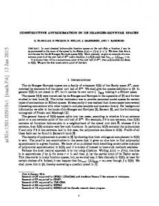
 t?t=2 e?1=2ee?1=e: Then use 1 < t < 2 to complete the proof. ut These estimates are compared in Figure 2.

Lemma B.4. Let (u) be the modulus of smoothness of a Banach space, and assume that (u)  ut for all u  0 (t 2 [1; 2] is xed). Then 1=t  (B.44) : 1 + 1 < 5t ? 1

2 (2 )1=t Proof. De ne h(t) to be the right-hand side of (B.44). Then the derivative of h(t) has the same sign as    5t ? 1 1 ? log 5t ? 1 + 1 : (B.45) 2 2 2 But (B.45) is decreasing in t for t > 3=5, so h0(t) = 0 for at most one point t0 2 [1; 2] (in fact t0  1:4724), which would be a local maximum for h. In particular, for any subinterval [t1; t2]  [1; 2], it must be that h(t)  min(h(t1 ); h(t2)) for all t 2 [t1; t2].

32

Donahue, Gurvits, Darken, and Sontag

1.0

1 [(2 ? t)t]1?t=2 (t ? 1)t?1 t

p

2?1 3?t=2 2t?1=5t=2 1 e?3=2e t

0.8 0.6 0.4 0.2 0.0 1.0

1.2

1.4

1.6

1.8

2.0

Fig. 2. Comparison of lower bound estimates on (from Lemma B.3) as a function of t. For our purposes we divide the interval [1; 2] into two subintervals: [1; 5=4] and [5=4; 2]. Evaluating h at the endpoints yields h(1) = 2 h(5=4) = (21=8)4=5 > 2:16 p h(2) = 3= 2 > 2:12: Therefore h(t)  2 for t 2 [1; 5=4], and h(t)  2:12 for t 2 [5=4; 2]. To obtain the corresponding upper bounds on the left-hand side of (B.44), apply (B.39) for t 2 [1; 5=4], and (B.40) for t 2 [5=4; 2]. ut

C. A Sequence Inequality The following lemma may be viewed as pertaining to a discrete analogue of the dierential equation y0 = y1?t , the general solution of which is y(x) = (tx+C)1=t. It can be used to provide bounds on the convergence rate of sequences having incremental changes compatible with the estimates from Lemma 3.3, with which it is combined to produce Theorems 3.5 and 3.7. Lemma C.1. Let (an ) be a nonnegative sequence satisfying 3 1  (C.46) an+1  an + min 2 ; t?1 an

Rates of Convex Approximation

for all n, where 1  t  2. If

(C.47)

33

1=t



an  tn + t ?2 1 log2 n

is satis ed for some n  2, or for n = 1 with a1  1, then it is satis ed for all n0 > n as well.

Proof. Let us take bn := tn + (1=2)(t ? 1) log2 n, assume that an  b1n=t, and proceed by induction, i.e., show that an+1  b1n=t+1. Suppose rst that an < 1 and n  2. Then b1n=t+1  b13=t  (6 + (1=2) log2 3)1=2 > 5=2: The second inequality holds because the function t 7! (3t+(1=2)(t ? 1) log2 3)1=t is decreasing in t for t 2 [1; 2], and so attains its minimum at t = 2. But then an+1  an + 3=2 < 5=2 < b1n=t+1 ; as desired. Alternatively, suppose that an  1. Then since the function x 7! x(1 + 1=xt) is nondecreasing for x  1, we have an+1  an(1 + 1=atn)  b1n=t(1 + 1=bn) 1=t   b1n=t 1 + bt + t(t2b?2 1) n n  ? 1 ? t ? 1 log (1 + 1=n)1=t :  t(n + 1) + t ?2 1 log2 (n + 1) + t 2n 2 2 The third inequality above follows from a Taylor series expansion of (1+1=bn )t . Combining this with the de nition of bn+1 and the fact that log2 (1 + 1=n)  1=n for n  1 yields an+1  b1n=t+1 ; concluding the proof.

ut

D. An Example of a Smooth Banach Space with Non-Converging -Greedy Sequences In Sect. 3.1 it was shown that P -greedy sequences in uniformly smooth spaces always converge (provided k < 1), and that smoothness is necessary and suf cient for monotonically decreasing error in incremental approximants. We now construct an example showing that simple smoothness is insucient to guarantee convergence of -greedy sequences.

34

Donahue, Gurvits, Darken, and Sontag

Let a = (a(n)) be a sequence of real numbers. De ne the sequence of functions (Fn ) (the norm sequence ) from IRIN to IR+ [ f0g recursively by F1(a) = ja(1)j Fn(a) = [(Fn?1(a))pn + ja(n)jpn ]1=pn ; where (pn ) is a xed sequence (called the norm power sequence ) with 1  pn < 1 for all n. Note that for each a, Fn(a) is nondecreasing with n. De ne (D.48)





X(pn ) := a 2 IR j sup Fn(a) < 1 ; IN

n

and for a 2 X(pn ) (D.49) kak := F(a) := nlim !1 Fn(a): The reader may verify that X(pn ) equipped with the norm (D.49) is a Banach space. (This space is similar to the modular sequence spaces studied in (Woo 1973).) If (pn ) is bounded and pn > 1 for all n, then it can be shown that X(pn ) is smooth. Let us use the notation en 2 X(pn ) to denote the canonical basis element en (k) = n (k). (Note that kenk = 1 for all n independent of (pn ).) PropositionD.1. Let ( n) be a strictly decreasing sequence converging to 1. Then there exists a norm power sequence (pn ) that is non-increasing, converges to 1, and has pn > 1 for all n, such that the bounded set S = f? 1 e1 g [ f n en gn2IN in X(pn ) admits for each incremental schedule (n ) an incremental sequence (an )  coS that is -greedy with respect to 0 but does not converge. (Note that 0 2 coS .) Proof. X(pn ) is determined by its power sequence (pn). Choose p1 > 1 arbitrarily, and recursively select pn 2 (1; pn?1] to satisfy inf [(1 ? ) n?1 ]pn + ( n )pn > 1: (D.50) 01 This can always be done because the inequality holds for pn = 1 and so by continuity in pn holds also for all pn suciently close to 1. Now let (k ) be a xed incremental schedule. We build an -greedy (with respect to 0) sequence (ak )  S  coS as follows. Let a1 = n1 en1 be any 1greedy element of S with n1 > 1 (i.e., n1 < minf1 + 1; 1 g). Assuming that ak?1 = nk?1 enk?1 with nk?1 > 1, we will show that we can pick ak = nk enk with nk > nk?1 to be k -greedy. Indeed, suppose that bk = (1 ? )ak?1 + gk is an k -greedy step, where gk 2 S. It follows from (D.50) and the monotonicity of n that kbk k > 1, so we can pick nk > nk?1 such that kbk k > nk = k nk enk k: Therefore, taking ak = nk enk yields an k -greedy increment. We de ne the sequence (ak ) recursively in this manner to complete the construction. ut

Rates of Convex Approximation

35

References Banach, S., and S. Saks (1930) Sur la convergence forte dans les champs LP , Studia Math., 2:51{57. Barron, A. R. (1991) Approximation and estimation bounds for arti cial neural networks, in Proc. Fourth Annual Workshop on Computational Learning Theory, Morgan Kaufmann, 243{249. Barron, A. R. (1992) Neural net approximation, in Proc. of the Seventh Yale Workshop on Adaptive and Learning Systems, 69{72. Bessaga, C., and A. Pelczynski (1958) A generalization of results of R. C. James concerning absolute bases in Banach spaces, Studia Math., 17:151{164. Clarkson, J. A. (1936) Uniformly convex spaces, Trans. Amer. Math. Soc., 40:396{414. Darken, C., M. Donahue, L. Gurvits, and E. Sontag (1993) Rate of approximation results motivated by robust neural network learning, in Proc. of the Sixth Annual ACM Conference on Computational Learning Theory, The Association for Computing Machinery, New York, N.Y. 303{309. Deville, R., G. Godefroy, and V. Zizler (1993) Smoothness and Renormings in Banach Spaces. Wiley, N.Y.. Dieudonne, J. (1960) Foundations of Modern Analysis. Academic Press, N.Y.. Figiel, T. and G. Pisier (1974) Series aleatoires dans les espaces uniformement convexes ou uniformement lisses, C. R. Acad. Sci. Paris, 279, Serie A:611{614. Gowers, W. T., A Banach space not containing c0 , l1 , or a re exive subspace. Preprint. Haagerup, U. (1982) The best constants in the Khintchine inequality, Studia Math., 70:231{ 283. Hanner, O. (1956) On the uniform convexity of Lp and `p , Arkiv for Matematik, 3:239{244. Hanson, S. J. and D. J. Burr (1988) Minkowski-r back-propagation: learning in connectionist models with non-Euclidean error signals, in Neural Information Processing Systems, American Institute of Physics, New York, 348. James, R. C. (1978) Nonre exive spaces of type 2, Israel J. Math., 30 :1{13. Jones, L. K. (1992) A simple lemma on greedy approximationin Hilbert space and convergence rates for projection pursuit regression and neural network training, Annals of Statistics, 20:608{613. Kakutani, S. (1938) Weak convergence in uniformly convex spaces, T^ohoku Math. J., 45:188{ 193. Khintchine, J. (1923) U ber die diadischen Bruche. Math. Z., 18:109-116. Ledoux, M. and M. Talagrand (1991) Probability in Banach Space. Springer-Verlag, Berlin. Leshno, M., V. Lin, A. Pinkus, and S. Schocken (1992) Multilayer feedforward networks with a non-polynomial activation function can approximate any function. Preprint. Hebrew University. Lindenstrauss, J. (1963) On the modulus of smoothness and divergent series in Banach spaces, The Michigan Math. J., 10:241{252. Lindenstrauss, J. and L. Tzafriri (1979) Classical Banach Spaces II: Function Spaces. SpringerVerlag, Berlin. Powell, M. J. D. (1981) Approximation theory and methods. Cambridge University Press, Cambridge. Rey, W. J. (1983) Introduction to Robust and Quasi-Robust Statistical Methods. SpringerVerlag, Berlin. Rosenthal, H. (1974) A characterization of Banach spaces containing l1 , Proc. Nat. Acad. Sci. (USA), 71:2411{2413. Rosenthal,H. (1994) A subsequence principle characterizingBanach spaces containing c0 , Bull. Amer. Math. Soc., 30:227{233. Sontag, E. D. (1992) Feedback stabilization using two-hidden-layer nets, IEEE Trans. Neural Networks, 3:981{990. Stromberg, K. R. (1981) An Introduction to Classical Real Analysis. Wadsworth, New York. Woo, J. Y. T. (1973) On modular sequence spaces, Studia Math., 48:271{289.

36

Donahue, Gurvits, Darken, and Sontag

Michael J. Donahue Institute for Mathematics and its Applications University of Minnesota Minneapolis, MN 55455

Leonid Gurvits Learning Systems Department Siemens Corporate Research, Inc. 755 College Road East Princeton, NJ 08540

Christian Darken Learning Systems Department Siemens Corporate Research, Inc. 755 College Road East Princeton, NJ 08540

Eduardo Sontag Department of Mathematics Rutgers University New Brunswick, NJ 08903

This article was processed using the LATEX macro package with CAP style