Michael A. Slawinski, Raphaël A. Slawinski and R. James Brown ...... Brown, R.J., Lawton, D.C., and Cheadle, S.P., 1991, Scaled physical modeling of ...
Energy partition at the boundary
Energy partition at the boundary between anisotropic media; Part two: Raytracing in layered, anisotropic media comparison of traveltimes for synthetic and experimental results Michael A. Slawinski, Raphaël A. Slawinski and R. James Brown ABSTRACT We present a ray-tracing method for layered, anisotropic media. The method is used to calculate traveltimes for a two-layer isotropic/anisotropic medium consisting of PVC and Phenolic CE. We compare the numerical results with experimental data, confirming the validity of the approach. Furthermore, the comparison illustrates that physical measurements of such a model are better described by the anisotropic approach than by the isotropic one. The usefulness of our method can be extended to various modelling schemes, nearsurface statics corrections, vertical-seismic-profile (VSP) studies and inversion. Equations used in ray tracing are, in general, analytic and can easily be coded. INTRODUCTION Slawinski and Slawinski (1994) presented an analytic “Snell’s law” formalism for anisotropic media in which all expressions are exact and can be applied in most circumstances. The fact that the phase-slowness surface is smooth and never has cusps (Winterstein, 1990) ensures the applicability of vector calculus methods required by the formalism. The direct use of this formalism requires an expression of slowness surfaces as functions of three Cartesian coordinates x, y, and z. Slowness surfaces are three-dimensional closed surfaces of various degrees of symmetry, reducing in the isotropic case to spheres. The choice of spherical coordinates for description of a slowness surface, or polar coordinates for description of a slowness curve, is natural. Thus instead of directing one’s efforts towards developing a method of expressing slowness surfaces or curves in Cartesian coordinates, or as parametric plots, another method is adopted. The formalism serves as a template for linking, through the relation between Cartesian and polar coordinates, the analytical method for calculating angle of transmission across an interface, with actual measures of anisotropy defining the materials. Most commonly they are expressed as elastic constants, Cij, the entries of a 6x6 stiffness matrix relating stress and strain vectors, i.e., the anisotropic form of Hooke’s law. Thomsen (1986) suggests particular combinations of elastic constants as convenient measures of anisotropy. They are referred to in this paper as anisotropic parameters, and are denoted by δ, ε and γ. The velocities of both compressional and shear waves can be expressed in terms of those parameters. If the anisotropy is not very pronounced the formulæ for phase velocities can be developed in Taylor series and higher-order terms ignored without significant loss of accuracy (Thomsen, 1986). In the geophysical context, this process can be justified by the fact that, although on a small scale many crystals are highly anisotropic, the rocks that they form exhibit, in general, only moderate anisotropy as perceived by a wavelet
CREWES Research Report – Volume 7 (1995)
9-1
Slawinski, Slawinski and Brown
of the relatively low frequencies typical in seismic studies. The phase-velocity formulæ for three wave types in weakly anisotropic media provide the expressions used in deriving the mathematically tractable, as well as easily coded, Snell’s law-or more properly, laws of reflection and refraction for such media, which are, of course, not embraced by Snell’s law. In principle, it is possible to use the exact formulæ for phase velocities derived by Daley and Hron (1977) and expressed in terms of anisotropic parameters by Thomsen (1986). The significant loss of clarity of development caused by employing such complicated equations was avoided by using, in their stead, the approximate equations governing weak anisotropy. It is the slowness surfaces which form the kernel of Snell’s law. Since the formulæ for phase slowness can be elegantly described in polar coordinates it is preferable to translate the earlier formalism to this system. The formulæ given below refer explicitly to propagation within a transversely isotropic (TI) system with a vertical symmetry axis (TIV), or in the symmetry plane of a given medium (e.g., an orthorhombic medium was used in laboratory measurements). The distinctive elastic properties of the TIV system are an infinitefold vertical axis of rotational symmetry, and an infinite set of two-fold horizontal symmetry axes (Winterstein, 1990). It is described by five independent elastic constants. A TIV system describes well the intrinsic anisotropy found in a horizontal sedimentary layer like a shale unit. Also, a series of isotropic layers of thickness considerably smaller than the wavelength exhibits, as a whole, TIV symmetry (e.g., Postma, 1955, Schoenberg, 1994). The assumption of weak anisotropy implies that for the compressional-wave solution, the divergence of displacement is much larger than its rotation; while for the shear-wave solutions, the rotation is much larger than the divergence (Helbig, 1994). Thus the solutions are only weakly coupled and the particle displacement is almost parallel (in the case of quasi-compressional waves) or almost orthogonal (in the case of quasi-shear waves) to the direction of propagation. It can be shown that the wave equation for transverse isotropy yields three independent solutions corresponding to mutually orthogonal polarization directions. The solutions refer to one quasi-longitudinal wave (qP), one quasi-transverse wave (qSV) and one exactly transverse wave (SH) (e.g., Keith and Crampin, 1977). Along the symmetry axis all polarizations become pure and all expressions reduce to the isotropic form. An important consequence of weak anisotropy in TI media is that it is reasonable to consider two separate cases: one involving P, SV and the other SH waves, respectively. The simplification of expressions for phase velocities is achieved by developing the original expressions in Taylor series and neglecting higher-order terms, under the assumption that the anisotropic parameters are much smaller than unity. Although the simplification of expressions is very considerable (Thomsen, 1986), the accuracy is very high as long as the weak-anisotropy assumption is not violated. Thank to this assumption and the ensuing simplifications, the entire mathematical treatment developed and used in this paper is tractable, and, in most practical situations, leads to analytical expressions. If any computational algorithm is to work for general anisotropy it must also work for weak anisotropy. Thus, a mathematically tractable approach provides a potential verification for a machine-intensive program which would use the full form of the equations for velocity anisotropy. The innovative aspect of the approach presented in
9-2
CREWES Research Report – Volume 7 (1995)
Energy partition at the boundary
this paper consists of a clear analytical method for calculating propagation angles across an interface in anisotropic media, with all quantities related to the set of measurable parameters proposed by Thomsen (1986) and widely used by numerous researchers (e.g., Stewart, 1988, Cheadle et al., 1991, Brown et al., 1991). Except for using the weak-anisotropy form of the expression for phase velocity, the present method makes no simplifications or approximations in deriving the reflection/refraction expressions for weakly anisotropic media. QUASI-COMPRESSIONAL WAVES Phase velocity The phase velocity of a quasi-compressional, qP, wave in a weakly anisotropic medium is given by Thomsen (1986) as: v qP (ξ ) = α 0 (1 + δ sin 2 ξ cos2 ξ + ε cos4 ξ ) .
(1)
In this paper the phase angle, ξ, is the phase latitude, and a complement of the Thomsen’s angle, θ, which is equivalent to the phase colatitude, i.e.,
ξ = π / 2 −θ ,
(2)
thus changing in some equations, cosine function to sine function. In this form, one can take advantage of standard vector-calculus expressions in polar coordinates, in which the argument is measured with respect to the horizontal axis. Thus the gradient can be expressed as follows: ∇f (r , ξ ) = r
∂f 1 ∂f +Ξ , ∂r r ∂ξ
(3)
where the angle, ξ, is measured with respect to the x-axis. The anisotropic parameters used in the expression for phase velocity are defined in terms of either elastic constants, Cij, or measured velocities. The latter definition proves very helpful in experimental studies, e.g., Cheadle et al. (1991). From the experimental point of view, one ideally should have expressions for the anisotropy parameters in terms of both group and phase velocities, though one can always make do with the latter. In the laboratory, if anisotropy is sufficiently weak and transducer separation sufficiently small in relation to the diameters of the transducers, then one measures phase traveltimes (Dellinger and Vernik, 1994; Vestrum et al., 1996). If the anisotropy is sufficiently strong and the transducer separation sufficiently large in relation to their diameter, then one can determine group traveltimes. With any given sample, one can practically always cut as small a piece as is necessary to achieve phase-traveltime measurement. In either case, it is important to be aware what type of velocity one is measuring (Vestrum, 1994). For the parameters δ and ε relevant to qP-wave propagation:
CREWES Research Report – Volume 7 (1995)
9-3
Slawinski, Slawinski and Brown
δ≡
V (π / 4) V P (π / 2) (C13 + C44 ) 2 − (C33 − C44 ) 2 ≈ 4 P − 1 − − 1 , 2C33 (C33 − C44 ) V P (0) V P (0)
(4)
and
ε≡
C11 − C33 V P (π / 2) − V P (0) ≈ , 2C33 V P (0)
(5)
where Cij are entries in the stiffness matrix relating the six components of stress to the six components of strain, and VP denotes measured velocity. Sometimes, in these weak-anisotropy approximations involving “measured velocity”, either group or phase velocity will do more or less equally well and often, in practice, the experimentally observed traveltimes divided into the transducer separation would suffice without rigorous regard for the group/phase question. For deriving anisotropic parameters from actual measurements, however, it is advisable to use exact equations instead of their approximate counterparts. Particularly δ is prone to the propagation of experimental errors in its approximate form (Thomsen, 1986; Brown et al., 1991). The symbol αo denotes the speed of a ray propagating vertically, along the symmetry axis of the medium. It can be expressed in terms of an elastic constant or, similarly to the isotropic case, in terms of the Lamé parameters, λ, µ, and the density of the medium, ρ; that is:
α0 =
C33 = ρ
λ + 2µ . ρ
(6)
Notice that, for a ray propagating vertically, or horizontally, the phase and group velocities coincide, both in exact and approximate expressions. This is not necessarily the case in any other direction of propagation and it is important to distinguish between the two concepts. Transmission angle The subsequent development follows the formalism developed by Slawinski and Slawinski (1994). Firstly, one must formulate an expression for a slowness surface. The phase slowness is the reciprocal of the phase velocity, obtained by taking reciprocals of all points on the phase velocity surface (e.g., Winterstein, 1990). Thus, the slowness surface is given by a level surface defined by the inverse of the phase velocity function. Let f(r,ξ) be a function in slowness space defined by: f (r , ξ ) =
1 − α 0 (δ sin 2 ξ cos 2 ξ + ε cos4 ξ ) , r
(7)
where r is the radius of the slowness surface, i.e., the magnitude of the slowness. Similarly, working in slowness space, x, y and z are the Cartesian components of slowness (cf. Slawinski and Slawinski, 1994).
9-4
CREWES Research Report – Volume 7 (1995)
Energy partition at the boundary
For a particular TI medium, its slowness as a function of ξ is r(ξ) which is given by equation (16). This set of points [r(ξ),ξ] is also given by the intersection of f(r, ξ) with the plane f = αo, i.e., by the set of points (r, ξ) for which: f (r , ξ ) = α 0 .
(8)
The ray (group) vector is always perpendicular to the slowness surface, i.e., its direction is parallel to the gradient of the slowness surface. Using calculus and various trigonometric identities, the gradient of f(r, ξ) can be written as follows:
[
α 0 sin(2ξ ) δ cos(2ξ ) − 2ε cos 2 ξ ∂f 1 ∂f 1 ∇f (r , ξ ) = r +Ξ = r − 2 + Ξ r ∂r r ∂z r
] , (9)
where r is the unit radius vector and Ξ is the unit azimuthal vector. The length of the gradient is: 2
1 ∂f 1 1 ∂f ∇f = + + α 0 sin(2ξ ) δ cos(2ξ ) − 2ε cos 2 ξ ] = ∂r r r2 r ∂ξ 2
(
])
[
2
. (10)
Thus the unit ray vector, w, in the direction of the ray is [Slawinski and Slawinski, 1994; equation (11)]: w=
∇f . ∇f
(11)
The angle between the unit ray vector, w, and the normal can be found using the definition of the dot product. Using the vertical unit vector, z, one may write: cosθ = z ⋅ w .
(12)
In polar coordinates, the Cartesian unit vector, z, can be expressed in terms of its relation to the radius r and the argument angle ξ. In the present context the argument corresponds to the phase angle, i.e.: z = r sin ξ + Ξ cos ξ .
(13)
This form is used in the desired dot product. Combining equations (9) through (13), one can express the group angle, θt, which the group slowness vector of a transmitted ray makes with the normal to the interface, in terms of the phase angle, ξ, measured from the horizontal as:
(
)
α 0 cos ξ sin(2ξ ) δ cos(2ξ ) − 2ε cos2 ξ − cosθ t = z ⋅ w =
sin ξ r (ξ )
1 + [α 0 sin(2ξ )(δ cos(2ξ ) − 2ε cos2 ξ ]2 2 [r (ξ )]
.
(14)
In relating the incidence angle to the transmission angle one uses the fact that, for horizontal interfaces, the horizontal component of slowness, xo, i.e., the ray
CREWES Research Report – Volume 7 (1995)
9-5
Slawinski, Slawinski and Brown
parameter, must be constant. If the medium of incidence is isotropic than phase and group angles (and velocities) coincide. The horizontal component of slowness can be calculated, given the angle of incidence, from: xi =
sin θ i ≡ x0 , v
(15)
where the angle of incidence, θi, is measured from the vertical, and v is the speed in the isotropic medium of incidence. The radius of the cross-section of the qP-slowness surface(i.e., the slowness) for the anisotropic medium of transmission in the xz-plane is given by the inverse of the phase velocity: r(ξ ) =
1 , α 0 (1 + δ sin ξ cos2 ξ + ε cos4 ξ ) 2
(16)
and the horizontal component of slowness at a given point on a slowness surface is given by: x (ξ ) = r (ξ ) cos ξ .
(17)
Inserting equation (16) into equation (17) gives a relationship between the horizontal component of slowness, i.e., the ray parameter, xo, and the slowness surface for compressional waves; namely: x(ξ ) =
cos ξ . α 0 (1 + δ sin ξ cos2 ξ + ε cos4 ξ ) 2
(18)
Equation (18) can be rewritten as a quartic in cosξ and solved explicitly for the phase angle, ξ. Given the incidence angle, θi, and thus the ray parameter, x0, one obtains:
α 0 x 0 (ε − δ ) cos4 ξ + α 0 x 0δ cos2 ξ − cos ξ + α 0 x 0 = 0 .
(19)
The appropriate value of ξ can be inserted in equations (14) and (16) and the angle of transmission calculated. An insightful look into the solution of the quartic equation is given in this volume by Slawinski (1995). Note that in the case of elliptical anisotropy, i.e., ε = δ, the quartic is reduced to a quadratic of the form analogous to the equation for SH-waves. Also note that, in all expressions, θ is the group (ray) angle measured with respect to the normal to the interface, and ξ is the phase angle measured with respect to the horizontal. RAY TRACING An important element of studying wave propagation consists of the ability of predicting theoretically the results which one would obtain by measuring, at a given receiver, a signal emitted by a distant source. A powerful and rather intuitive technique for this purpose is provided by the ray theory. This is an approximation to the full-wave theory and derives from the approach used in geometrical optics. With the aid of Snell’s law, using ray-tracing theory and knowing all parameters of the medium, one can calculate the trajectory of a ray between the source and receiver, as
9-6
CREWES Research Report – Volume 7 (1995)
Energy partition at the boundary
well as the traveltime required. This is a, so called, forward problem or forward modelling: one calculates the “observed” results knowing all parameters. Ray-tracing concepts The crucial point of ray tracing between a given source and receiver consists of finding the incidence angle which, in combination with transmitted angles, and obeying Snell’s law at all interfaces, yields the raypath corresponding to a given source-receiver distance. This is, as a matter of fact, a little inverse problem, here used in the larger context of forward modelling. The required equation for a two-layer case, can be written as follows: X1 + X 2 = X ,
(20)
i.e., the sum of horizontal distances travelled in the first, X1, and the second, X2, layer, must equal the total horizontal distance between the source and receiver, X. In terms of layer thicknesses, h1 and h2, as well as angles of incidence, θi, and transmission, θt, this can be written as: h1 tan θ 1 + h2 tan θ 2 = X ,
(21)
or in terms of angle of incidence: h1 tan θ i + h2 tan[θ t (θ i )] = X ,
(22)
where the expression in square brackets, i.e., angle of transmission as a function of the angle of incidence, is a concise statement of Snell’s law. Overview of the ray-tracing algorithm The ray tracing algorithm has been implemented using Mathematica software (Wolfram, 1991). The software was used to solve the quartic under the constraints provided by source and receiver locations, and the parameters of the medium. The algorithm was tailored specifically to the experiment, i.e., a two-layer case: isotropic/anisotropic. The algorithm can be described in the following way: - Firstly, a “take-off” angle is calculated by solving equation (22) for a given source-receiver separation. It is impossible to solve such an equation explicitly for θi, and therefore a root-finding routine is employed. The anisotropic formulation of transmission angle is honoured in the search for the “take-off” angle. In the process of finding, θi, which in the isotropic medium of incidence corresponds to both phase and group angles, the values of phase and group angles, ξ and θ, in the medium of transmission are established. - Secondly, the magnitude of group velocity corresponding to the ray exhibiting the angles calculated in the step above is calculated in both media. Again, the process is facilitated by the fact that in the isotropic medium of incidence the notions of phase and group velocity coincide and, as a matter of fact, by the very definition of isotropy, their magnitudes are constant.
CREWES Research Report – Volume 7 (1995)
9-7
Slawinski, Slawinski and Brown
- Thirdly, the distances travelled by a signal in either medium are calculated based on layer thicknesses, source-receiver distance, and group angles. Subsequently, the traveltime is computed, i.e., the ratio of distance travelled to group velocity. PHYSICAL MODELLING Physical modelling provides the results of controlled experiments, which can be compared with numerically obtained predictions. It provides an indication of the degree of correctness of the theoretical approach. In this study, laboratory measurements serve as a template to compare two approaches for ray tracing; namely the approach based on the weak-anisotropy assumption, and the more traditional approach, ignoring anisotropic effects. Such comparison, in practical consideration, can help one decide whether sufficient accuracy is achieved by a more straightforward isotropic approach or whether one should resort to a more complicated anisotropic approach. Materials The medium through which the signal is transmitted is composed of two layers. The model with its anisotropic parameters in the 31-plane was considered as a standard model. The top, isotropic, layer consists of PVC and the lower, anisotropic layer of Phenolic CE. The CE-grade phenolic laminate is composed of layers of a woven canvas fabric saturated and bonded with phenolic resin. The woven pattern results in anisotropic symmetry. Former studies (e.g., Cheadle et al., 1991; Brown et al., 1991; Vestrum, 1994) have shown that Phenolic CE can be classified as belonging to the orthorhombic symmetry group. Experiments were conducted with the 31-plane as a saggital plane (Cheadle et al., 1991). Principal dimensions and quantities are shown in Tables 1, 2 and 3. Layer # 1 2
Material PCV Phenolic CE
Thickness (m) 0.0355 m 0.1045 m
Symmetry Class isotropic orthorhombic
Table 1. The principle dimensions and characteristics of the model
Layer # / Symmetry plane 1/ isotropic 2 / (31-plane)
Vertical P-wave speed (m/s) 2250 2925 Table 2. Vertical or isotropic speeds of the model
The values of the anisotropic parameters result from experimental measurements on the very same material performed in the same laboratory setting and reported by
9-8
CREWES Research Report – Volume 7 (1995)
Energy partition at the boundary
Cheadle et al. (1991). Vestrum (1994).
The results were confirmed by the subsequent study of
Layer # / Symmetry plane 1 2 / (31-plane)
δ
ε
0 0.183
0 0.224
Table 3. Anisotropic parameters of the model.
Experimental setup The data were recorded using two transducers of 1-MHz frequency, one being a transmitter, the other a receiver. The transmitter was fixed in one location, while the receiver was moved along the straight line containing the symmetry plane. The readings were taken every millimetre in a horizontal range from 0 mm to 300 mm. The apparatus used in the data acquisition is a converted high-precision plotter. The entire acquisition process is performed automatically.
X (source-receiver distance ) transmitter PVC 0.0355 m
Phenolic CE
0.1045 m
receiver
Fig. 1. A schematic diagram of the experimental set-up.
Data analysis Recorded signal was plotted as a standard seismic display. In order to use standard plotting devices, as well as to render the results more immediately applicable to a geophysical context, the distances were scaled by a factor of 10,000. This also implies that traveltime values are scaled by the same factor.
CREWES Research Report – Volume 7 (1995)
9-9
Slawinski, Slawinski and Brown
The case of transmitted and received compressional waves served as a test for the predictive power of raytracing procedures described in this paper. This case, as opposed to SV or SH waves, was selected as giving the cleanest first breaks because the compressional waves are the first to arrive at the receiver. The results show that, as expected, the raytracing incorporating the anisotropic effects predicts better the experimental results. Scaled offset (m)
0 190 390 590 790 990 1190
Traveltime in 31-plane (s) calculated measured (anisotropic) αo= 2925 m/s δ = 0.183 ε = 0.224 0.515385 0.516 0.518585 0.519 0.528745 0.528 0.545512 0.544 0.568328 0.569 0.596497 0.601 0.629263 0.635
Traveltime (s) calculated (isotropic) v = 2925 m/s
0.515385 0.519702 0.534388 0.558283 0.590214 0.628889 0.673073
Table 4. Traveltimes for P-waves; the calculated values are based on the anisotropic approach using values of anisotropic parameters published by Cheadle et al. (1991).
The calculation based on the anisotropic approach using the values of anisotropic parameters published for the block of Phenolic CE by Cheadle et al. (1991) approximates the measured times much more closely than the calculation based on the isotropic approach (see Table 4 and Figure 2). This confirms that the anisotropic approaches reflects better the reality of the experiment. In the context of exploration geophysics, it implies that in certain areas one might consider analysis of the data that takes anisotropy into account. CONCLUSIONS: PRACTICAL APPLICATIONS Modelling A reliable method allowing one to generate synthetically the experimental results can play a very important rôle. Such a technique incorporated into the planning of a seismic experiment, allows one to anticipate the results and thus to correctly deploy sources, receivers, and other experimental apparatus. Furthermore, it allows the interpreter to verify (while keeping in mind the intrinsic non-uniqueness) the results of interpretation by comparing synthetic data, generated based on a given interpretation, with experimental results.
9-10
CREWES Research Report – Volume 7 (1995)
Energy partition at the boundary
P-P waves in 31-plane 0.7 calculated
traveltime (s)
0.65
measured isotropic
0.6 0.55 0.5 0.45 0.4 0
190
390
590
790
990
1190
offset (m)
Fig.2. A graphical comparison of results for compressional (P-P) waves in the 31-plane. Note the excellent fit between measured traveltimes (squares) and traveltimes calculated using “anisotropic” raytracing (diamonds). Also note that results obtained using “isotropic” raytracing (triangles) depart increasingly from the measured data with increasing offset within the range typical in exploration geophysics.
The ray-tracing method presented here allows one to generate synthetically results of wave propagation in layered weakly anisotropic media. Although the present paper concentrates on compressional waves and a two-layer isotropic/anisotropic case, the method has been elaborated to include both compressional and shear waves in multilayer anisotropic media. The ray-tracing method presented can serve as the basis of decision as to whether or not an ”anisotropic” approach should be followed. The degree of anisotropy can be varied by modifying anisotropic parameters and the discrepancy between isotropic and anisotropic approaches investigated. As indicated by physical experiments, the anisotropic-modelling approach reflects very closely the experimental results; one should, however, keep in mind that the algorithm is designed for weakly anisotropic media, and the accuracy of results relies on this assumption. As a reasonable rule one can accept degree of anisotropy of about 20% as being the limit of applicability. Near-surface static corrections Calculation of static corrections, dealing with shallow reflections and refractions, employ obliquely traveling rays. For such rays the effects of anisotropy are, in general, more pronounced than for deep reflections for which all rays are nearly vertical. Furthermore, large differences in velocities among near-surface layers emphasize the raybending at interfaces, calling for an accurate description of this phenomenon.
CREWES Research Report – Volume 7 (1995)
9-11
Slawinski, Slawinski and Brown
The anisotropic ray tracing presented in this paper allows one to calculate static corrections including the effects of anisotropy. For instance, it is important to realize that the value of the critical angle is not the same for isotropic and anisotropic cases, thus directly affecting results of refraction statics. Vertical seismic profiling (VSP) The recording geometry of an offset-VSP, with receivers deployed throughout a long section of the wellbore and the source located on the surface at a considerable lateral distance from the well, can be particularly affected by anisotropic effects. The data set comprises propagation directions ranging from nearly vertical to nearly horizontal, thus giving the opportunity for any angular dependence to manifest itself. Assuming that the anisotropy of the rock mass can be characterized as a TIV system, i.e., transverse isotropy with the vertical symmetry axis, and the geological layering is approximately horizontal, the VSP geometry is ideally suited for employing the method presented in this paper. As a matter of general practice, in addition to the offset source, one [often, usually] records with a zero-offset source. For the latter case the rays travel nearly vertically and, since the distance traveled is measured by the geophone cable, the traveltime reliably yields the vertical speed, a0, required by the formalism. Subsequently, by modifying anisotropic parameters, d and e, one can fit modelled and actual data. Furthermore, VSP geometry provides an excellent experimental setup for traveltime inversion, which can yield the anisotropic parameters. As already mentioned, this geometry gives reliable information on the vertical speed from the zero-offset record and on the angle-dependent traveltime measurements from the faroffset record. Moreover, the presence of the wellbore provides information about thicknesses of sedimentary layers. Inversion The ray-tracing method presented in this paper forms the basis of an inversion method which yields the values of anisotropic parameters based on measurements of traveltime. An analytical traveltime inversion has been formulated and successfully tested for SH waves. ACKNOWLEDGMENTS The authors would like to thank Eric Gallant for performing all laboratory experiments, including the design and building of the experimental apparatus and the CREWES’ sponsors for their generous support. REFERENCES Brown, R.J., Lawton, D.C., and Cheadle, S.P., 1991, Scaled physical modeling of anisotropic wave propagation: multioffset profiles over an orthorhombic medium: Geophys. J. Int. 107, 693702. Cheadle, S.P., Brown, R.J., and Lawton, D.C., 1991, Orthorhombic anisotropy: a physical seismic modeling study: Geophysics, 56, 1603-1613.
9-12
CREWES Research Report – Volume 7 (1995)
Energy partition at the boundary
Daley, P.F., and Hron, F., 1977, Reflection and transmission coefficients for transversely isotropic media: Bull., Seis. Soc. Am., 67, 661-675. Dellinger, J., and Vernik, L., 1994, Do traveltimes in pulse-transmission experiments yield anisotropic group or phase velocities?: Geophysics, 59, 1774-1779. Helbig, K., 1994, Foundations of anisotropy for exploration seismics: Pergamon. Postma, G.W., 1955, Wave propagation in a stratified medium: Geophysics, 20, 294-392. Schoenberg, M., 1994, Transversely isotropic media equivalent to thin isotropic layers: Geophys. Prosp., 42, 885-915. Slawinski, M.A., and Slawinski, R.A., 1994, Energy partition at the boundary between anisotropic media; Part one: Generalized Snell’s law: CREWES Research Report, 6, 9.1-9.12. Slawinski, M.A., 1995, The characteristic biquadratic: An illustration of transmission in anisotropic media: CREWES Research Report, 7, 9.1-9.5. Stewart, R.R., 1988, An algebraic reconstruction technique for weakly anisotropic velocity: Geophysics, 53, 1613-1615. Thomsen, L., 1986, Weak elastic anisotropy: Geophysics, 51, 1954-1966. Vestrum, R.W., 1994, Group- and phase-velocity inversion for the general anisotropic stiffness tensor: M. Sc. thesis, Univ. of Calgary. Vestrum, R.W., Brown, R.J. and Easley, D.T., 1996, From group or phase velocities to the general anisotropic stiffness tensor: Proc. 6th Internat. Workshop Seismic Anisotropy, Trondheim, Soc. Expl. Geophys. (in press). Winterstein, D.F., 1990, Velocity anisotropy terminology for geophysicists: Geophysics, 55, 10701088. Wolfram, S., 1991, Mathematica, a system for doing mathematics by computer, 2nd edition: AddisonWesley Publishing Company, Inc.,
CREWES Research Report – Volume 7 (1995)
9-13
Slawinski, Slawinski and Brown
9-14
CREWES Research Report – Volume 7 (1995)