. the mapper will output the three tuples The resources will be grouped together during the reduce phase. First the reducer assigns an unique number to each of the resources. Then it iterates over the values associated with the key and outputs a tuple having as key the number assigned to the resource and as value the one fetched from the iterator. The ids are assigned in a similar way than before, with the task id on the first 3 bytes and a local counter value in the last 4. With this approach we won’t assign consequent numbers because it can be that the number of input processed by the reducer is smaller than the numbers available in the range. However this is not a big issue because: first, we are more interested in compressing the output than in building a nice and efficient dictionary and second, we can limitate the gap between the partitions choosing a range that is as close as possible to the real size of the reducer’s input so that there are only few numbers left out. The algorithm is reported in Algorithm 2.
32CHAPTER 4. DICTIONARY ENCODING AS MAPREDUCE FUNCTIONS Algorithm 2 Dictionary encoding: first job map( key , v a l u e ) : // key : i r r e l e v a n t // v a l u e : t r i p l e i n N−t r i p l e s f o rm a t local counter = local counter + 1 t r i p l e i d = t a s k i d in f i r s t 3 b y t e s resources [ ] = s p l i t ( value ) output . c o l l e c t ( r e s o u r c e [ 0 ] , t r i p l e i d output . c o l l e c t ( r e s o u r c e [ 1 ] , t r i p l e i d output . c o l l e c t ( r e s o u r c e [ 2 ] , t r i p l e i d
+ local counter + subject ) + predicate ) + object )
reduce ( key , i t e r a t o r v a l u e s ) : // I a s s i g n an u n i q u e i d t o t h e r e s o u r c e i n ’ key ’ local counter = local counter + 1 r e s o u r c e i d = t a s k i d in f i r s t 3 b y t e s + l o c a l c o u n t e r f o r ( v a l u e in v a l u e s ) output ( r e s o u r c e i d , i t r next )
The tuples in output contains the relations between the resources and the triples. The only moment when we have access to the resource both as number and as text is during the execution of the reducer task, therefore here we must take care of building the dictionary that contains the association . The dictionary can be stored in a distributed hash table, in a mysql database or simply in some separated files. If we do not store the dictionary we won’t be able to decode the triples to their original format.
4.4.3
Second job: rewrite the triples
This second job is easier and faster to execute than the previous one. The mapper reads the output of the previous job and swap the key with the value and it sets as the tuple’s key the triple id and as value the resource id plus the resource position. In the reduce phase the triples will be grouped together because the triple id is the tuple’s key. The reducer simply scrolls through the values and rebuild the triples using the information contained in the resource id and position. In our implementation the triples are stored in a Java object that contains the subject, the predicate and the object represented by long numbers. The object takes 24 bytes of space to store the resources plus one byte to record if the object is a literal or not. That means that one triple can be stored on disk with only 25 bytes. There are 800 million of triples, therefore the uncompressed encoded version requires only 19GB to be stored, against the 150GB necessary
4.4. DICTIONARY ENCODING USING ONLY MAPREDUCE
33
Algorithm 3 Dictionary encoding: second job map( key , v a l u e ) : // key : r e s o u r c e i d // v a l u e : t r i p l e i d + p o s i t i o n output . c o l l e c t ( v a l u e . t r i p l e i d , key + v a l u e . p o s i t i o n ) reduce ( key , i t e r a t o r v a l u e s ) : f o r ( v a l u e in v a l u e s ) i f v a l u e . p o s i t i o n = s u b j e c t do subject = value . resource i f v a l u e . p o s i t i o n = p r e d i c a t e do predicate = value . resource i f p o s i t i o n = o b j e c t n o t l i t e r a l do object = value . resource object literal = false i f p o s i t i o n = o b j e c t l i t e r a l do object = value . resource o b j e c t l i t e r a l = true output ( n u l l , t r i p l e ( subject , predicate , object , o b j e c t l i t e r a l ))
to store the triples in the original format. Using this technique the compression level is about 1:8.
4.4.4
Using a cache to prevent load balancing
The first job can suffer of a load balancing problem that can slow down the computation. If a particular resource is very popular there will be many intermediate tuples with the same key and all of them will be sent and processed by a single reducer task that is executed on a single machine. This load balancing problem is limited by the fact that we send only the triple id and not the complete triple as value, so that even the reducer has to process more values these are just 8 bytes each, so that the difference is still little. If the frequency of the nodes is spread uniformly the difference is not noticeable but if there are few extremely popular resource then the problem arises also if we just use numbers. To solve this problem we can initially identify which resources are extremely popular and prevent by being processed by a single reducer task. We can identify the popular resources by launching a job that counts the occurrences of the resources in the data. After we have done it we can, manually or with a script, assign a number to the most popular resources and store this association in a small text file. This file can be loaded by the mapper and kept in memory in a hash table as
34CHAPTER 4. DICTIONARY ENCODING AS MAPREDUCE FUNCTIONS a in-memory cache. Before the mappers output the tuples they check whether the resources are present in this hash table. If they are, instead of setting the resources as key they set a specific fake key of the form: "@FAKE" + random_data + "-" + ID_MANUALLY_ASSIGNED The random data prevents that all the tuples with the same ID end in the same reducer. When the reducer assigns a number to the key it checks first if the key starts with “@FAKE” and if it does it simply extracts the end of the string and use that number instead of a new one. In this way we assure that all those resources will get the same number even if they are processed by different reducers. Using the cache we greatly decrease the impact of load balancing with the effect of speed up the computation.
Chapter 5
RDFS reasoning as MapReduce functions In section 2.4.1 we described the theory behind RDFS reasoning. We defined it as a process in which we keep applying certain rules to the input set until we reach a fix point. The RDFS reasoning can be done in different ways. The development process of the algorithm started with a very simple and dummy implementation and it went through many changes until it ended in a final and tested version. This section describes three possible algorithms starting from the first naive one and ending in a more refined and optimized version. This explanation reflects the development process of the program that was developed along with this work. The first two versions are no longer present in the current code because they are obsolete and inefficients. The third and final algorithm is described more in detail and it is the one used to evaluate the performances of our approach.
5.1
Excluding uninteresting rules
The RDFS reasoner consists in a ruleset of 14 rules (reported in table 2.1) that we have to apply to the dataset. In this ruleset there are certain rules that are trivial and uninteresting and we will exclude them from our discussion. Those rules are rule number 1,4a,4b,6 and 10. The decision of leaving them out lies on the fact that they produce a trivial output that cannot be used for further derivations. Said in other words, they do not produce information that is usable for our reasoning purposes. These rules work using only one triple in input and, in case the user requires the reasoner to behave as a standard RDFS reasoner (therefore returning also this trivial output), we can easily implemented by simply apply a single and load balanced MapReduce job at the end of the computation. To explain better why these rules are unimportant let’s take for example the 35
36
CHAPTER 5. RDFS REASONING AS MAPREDUCE FUNCTIONS
rules 4a and 4b. Basically what these rules do is to explicitly mark any URI that is subject or object in a triple as a type of rdfs:Resource. These rules are trivial and indeed very easy to implement, but the output of them cannot be used for further derivation. The only rules that could fire using the output of rules 4a and 4b are rules 2,3,7 and 9 but they will never do. The reason stands on the fact that if we want that rules 2 and 3 fire then rdf:type must have a domain or a range associated with it. Also, if we want that rules 7 and 9 fire then rdf:type must be defined as a subproperty of something else or rdfs:Resource as a subclass of something else. Since both rdf:type and rdfs:Resource are standard URIs defined by the RDF language the user is not allowed to change their semantic adding custom domains or ranges or defining them as subclass of something else. If there are such triples in input they should be simply ignored because these are dangerous triples that try to redefine the standard language (more about ontology hijacking is said in section 3). If we assume the input data is clean and comply to the standard then rules 2,3,7 and 9 will never fire and we can safetly claim that rules 4a and 4b produce an output that cannot be used for further reasoning. The same motivation applies also for the other excluded rules. After we leave these uninteresting rules out, the ruleset becomes a subset made of 9 different rules.
5.2
Initial and naive implementation
In the program that we developed we first apply a technical job that converts the data in N-Triples format in a more convenient format for us. This job is not important for our reasoning task because it is strictly technical. The only thing it does is to convert the information in Java objects stored in files called “SequenceFile”. A “SequenceFile” is a file that stores the information as tuple of . Both the keys and values are particular Java objects that implement a specific Hadoop interface called “WritableComparable”. This interface defines some methods that the objects use to serialize themselves in a stream (that is a filestream in case of the SequenceFile). The advantage of storing the input data using a sequence file lies on the fact that Hadoop is able to automatically compress and decompress these files and it offers predefined input readers that read them in a transparent way. The information is already encoded as so the input can be read in a straightforward way without any conversion. In this initial version the reasoning is done by 9 different jobs, where each of them implements one rule. These jobs are repetitively launched until we reach a fix point. We will not describe all the single jobs because they are all very similar to each others. Instead we will just pick one rule and report a job as example.
5.2.1
Example reasoning job
The rule we take as example is:
5.3. SECOND IMPLEMENTATION
37
if a rdf:type B and B rfds:subClassOf C then a rdf:type C If we want to apply this rule we first need to search if there is a common element between any two triples in the input data. The triples must comply with the format written in the rule’s antecedents. In this particular example one triple must have as predicate the URI rdf:type while the second must have instead rdfs:subClassOf. The two triples must share at least one element, in this particular case the object of the first must be the same as the subject of the second. We can describe the reasoning as a process that first try to join different triples, and then, in case the join is possible, asserts of new information. If we see the derivation process under this point of view, we can rewrite the problem of applying a particular rule as the problem of finding all the possible joins between the information in the dataset. We can implement a data join for the rule we reported above with one MapReduce job. In such job the mapper checks whether the input triple is a “type” triple or a “subclass” triple. If it is a type triple it outputs a new tuple with as key the object of the triple and as value the triple itself. Instead, if it is a subclass triple, it outputs as key the triple’s subject instead of the object. The reducers will group the tuples according to their key. That means that if there are some “type” triples with the object equals to the subject of other “subclass” triples they will be grouped together. The reducer will iterate the list saving in memory the two types of triples in the group. It will then proceeds emitting the new derived information. We report the algorithm in Algorithm 4. All the nine different rules have the same structure: the mappers output the tuples using as keys the possible URIs that could be the match points. The reducers will check whether the match occurs and when it happens they will simply output the new information. There are many problems in this first implementation. The first and most important is a load balancing problem. If an URI is very popular and used in many joins then all the triples involved with that URI will be sent to a single reducer that must be able to store them in memory. Another problem relies on the fact that we need to launch a variable number of jobs depending on the input data. For example, if we take the subclass transitivity rule (the 11th rule in table 2.1), it will take logn jobs to derive everything if the input contains a subclass chain of n triples (a subclass b, b subclass c, c subclass d and so on). All of this makes the implementation unusable and indeed this version was abandoned almost immediately. The second implementation approaches the problem in a different way to overcome the two problems just illustrated above.
5.3
Second implementation
The main problems that were encountered for the previous implementation can be resumed in the list:
38
CHAPTER 5. RDFS REASONING AS MAPREDUCE FUNCTIONS
Algorithm 4 RDFS reasoning: example naive implementation map( key , v a l u e ) : // key : i r r e l e v a n t // v a l u e : t r i p l e i f v a l u e . p r e d i c a t e = r d f : type then output ( v a l u e . o b j e c t , v a l u e ) e l s e i f v a l u e . p r e d i c a t e = r d f s : s u b c l a s s then output ( v a l u e . s u b j e c t , v a l u e ) reduce ( key , i t e r a t o r v a l u e s ) : f o r t r i p l e in v a l u e s i f ( t r i p l e . p r e d i c a t e = r d f : type then t y p e s . add ( t r i p l e ) else s u b c l a s s e s . add ( t r i p l e ) f o r ( t y p e T r i p l e in t y p e s ) do f o r ( s u b c l a s s T r i p l e in s u b c l a s s e s ) do n e w T r i p l e = t y p e T r i p l e . s u b j e c t , r d f : type , s u b c l a s s T r i p l e . o b j e c t output ( n u l l , n e w T r i p l e )
• load balancing problem: doing a join in the reducer phase can be problematic in case there are very popular URIs shared by many triples; • complexity program: if there is even one single chain of subclasses in the data we need many more jobs to compute a complete closure. The second implementation solves these two problems rearranging the rule’s execution order and loading the schema triples in memory.
5.3.1
Rule’s execution order
We notice that all the nine rules output four different types of triple. Rules 5 and 12 output schema triples that define subproperty relations. All these triples can be distinguished by the others because they have rdfs:subPropertyOf as predicate. Rules 8, 11 and 13 return similar triples than the previous rules but with rdfs:subClassOf as predicate. Rules 2, 3 and 9 output data triples that define the type of some particular resources. All these triples share rdf:type as predicate. Only rule 7 outputs a triple that can be of every nature. If we look at the antecedents of the rules we are also able to make certain divisions. Rules 5 and 10 only work with schema triples that either define subclass of subproperty relations between the resources. Rules 8, 9, 12 and 13 work with a subset of the triples with (rdf:type), (rdfs:subClassOf ) or (rdfs:subPropertyOf )
5.3. SECOND IMPLEMENTATION
39
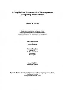
as predicate. Only rule 2, 3 and 7 can virtually accepts any triple in input. The relations between the rules are useful because if we launch the rules execution in a special order we can limitate the number of jobs that are necessary for the complete closure. Figure 5.1 reports the connection between these rules.
Figure 5.1: RDFS rules relations The ideal rule’s execution should start from the bottom of the picture and go to the top. That means we should first apply the transitivity rules (rule 5 and 11), then apply rule 7, then rule 2 and 3, then rule 9 and finally rules 8, 12 and 13. These three rules potentially can output triples that can be used by the initial transitivity rules but if we look more carefully we see than this is not the case. Rule 8 outputs a triple that could be used by rules 9 and 11. We exclude the case of rule 9 because the output would be that a resource x is type rdfs:Resource. This statement is valid for every resource and it can be derived also through rule 4a that is one rule that was excluded because trivial. Rule 8 could make rule 11 fire. We exclude the case that there is a superclass of rdfs:Resource because we assume that the schema may not be redefined, but it could be that there is a subclass of it. In this case we will materialize a statement that says that something is a subclass of rdfs:Resource. This statement cannot be used for any further derivation, therefore the cycle ends with it. Rule 12 outputs a triple of the form s rdfs:subPropertyOf rdfs:member. This could make rules 5 and 7 to fire. In both cases the output would be a triple that
40
CHAPTER 5. RDFS REASONING AS MAPREDUCE FUNCTIONS
cannot be used anymore. The same case is with rule 13. Rules 9 and 11 could fire but they would output either triples of the form s rdfs:subClassOf rdfs:Literal or s rdfs:type rdfs:Literal (the correctness of this last one is debatable since we are assuming that a resource is a Literal). Anyway in both cases these triples will not lead to any derivation. The most important consideration is that these last rules cannot generates a derivation that can make these rules firing again. In other words there is no main cycle in the rules execution. This consideration is important because we it means do not need to relaunch the same job more than once (except in the case the rule is recursive with itself). After we have applied rules 8, 12 and 13 we have reached a fixed point in our closure computation, because even we can derive some statements, those will not lead to any new derivation. In case we need to compute a complete RDFS closure, we can further process these last 3 rules, deriving the last statements and apply the trivial rules that we have excluded at the beginning of our discussion. This last part can be easily implemented, and therefore we will exclude it from our discussion. The only loops are the ones between the rules themselves. For example, if we want to apply rule 11, we need to apply it repetitively until we cannot derive anything anymore. Only after it we can safetly continue with our process. There are only 4 rules (rule 2, 3, 8, 12 and 13) that are not recursive. These inner loops are problematic because the numbers of repeats depends on the input data and we want to reduce the number of jobs to the minimum necessary. We solve this problem by loading some schema triples in memory.
5.3.2
Loading the schema triples in memory
We exploit the fact that the number of schema triples is much lower than the data triples and that all the joins we do are between a big subset containing the instance triples and a much smaller one containing the schema triples. For our rules we need four subsets of the schema triples. The first is the one that defines the domain of properties. This subset is used in rule 2. The second is the subset that defines the range of the properties. This is used in rule 3. The third is the one that defines the subproperty relation and it is needed in rules 5 and 7. The fourth and last is the set with the subclass relations used for rules 9 and 11. Since these four datasets are small we can store them in memory, and instead of doing the join using a single job as we did before we check if there is a match between the input triples with the triples that are kept in memory. For example if we want to apply the rule 9 we keep in memory all the triples that regard the subclass relations and, for every triple of the form a rdf:type B, we check if the triple’s object matches with one or more of the triples we keep in memory. If it does then we derive a new statement. We report a brief example to explain it better. Consider the set of input triples: a1 rdf:type A .
5.3. SECOND IMPLEMENTATION
41
b1 rdf:type B . A rdfs:subclassof B . B rdfs:subclassof C . C rdfs:subclassof D . The nodes load the “subclass” triples in a in-memory hash table with the subject of the triples as key and the object as value. Following the example this hash-map will contain the entries: key value A B B C C D When the mapper receives in input the triple a rdf:type A it checks whether there is a key equals to the triple’s object in the hash table. In this case the mapper succeed and the mapper fetches the value associated with A. This value is B and the mapper outputs the new triple a rdf:type B. The advantage of keeping the schema triples in memory is that we do not need to launch the job more than one time. In our previous approach we needed to launch the same job again and again until we reach a fixed point. If we keep the schema triples in memory we can check if there are matches in a recursive way. For example if we take rule 9 the output produced by applying the rule can be further used as input to check whether it could lead to a new derivation with the schema in memory. In this way we do not need to relaunch another job. After this last consideration we eliminate also the inner loops and our reasoning process becomes a linear sequence of jobs. In this implementation the join is done during the map phase. The reducers simply filter the derived triples against the input so that we avoid to write in output the same triple more than one time. The eight rules (rule 8 is not considered in this version) are implemented in two Hadoop jobs. The first job executes the two transitivity rules. The second applies all the other rules. In the next two subsections we describe these two jobs more in detail.
5.3.3
First job - apply transitivity rules
First we apply rules 5 and 11. These rules exploit the transitivity property of the subclass and subproperty relations making explicit every subproperty and subclass statement. The algorithm is reported in Algorithm 5. The mapper checks if the triple in input matches with the schema. In case it does, it simply emits the new derived triple, setting it as the tuple’s key, and setting true as value. It also outputs the input triple, with the only difference that it sets the value as false. The reducer code is very simple. It checks whether the triples in input are derived or not. It does that iterating over the values of the tuples. If there is a value set to false it means that the triple was present in input. In that case
42
CHAPTER 5. RDFS REASONING AS MAPREDUCE FUNCTIONS
Algorithm 5 RDFS reasoner: second version first job map( key , v a l u e ) : // key : i r r e l e v a n t // v a l u e : t r i p l e i f v a l u e . p r e d i c a t e = r d f s : s u b C l a s s O f then objects = subclass schema . r e c u r s i v e g e t ( value . object ) f o r o b j e c t in o b j e c t s output ( t r i p l e ( v a l u e . s u b j e c t , r d f s : subClassOf , o b j e c t ) , t r u e ) i f v a l u e . p r e d i c a t e = r d f s : subPropertyOf then s u p e r o b j e c t s = subprop schema . r e c u r s i v e g e t ( v a l u e . o b j e c t ) f o r ( o b j e c t in s u p e r o b j e c t s ) output ( t r i p l e ( v a l u e . s u b j e c t , r d f s : subPropertyOf , o b j e c t ) , t r u e ) output ( va lue , f a l s e ) reduce ( key , i t e r a t o r v a l u e s ) : f o r v a l u e in v a l u e s i f not v a l u e then exit output ( n u l l , key )
the triple is not outputted. Otherwise it is outputted only once. The reducer assures us we derive only unique triples.
5.3.4
Second job
The second job implements the remaining rules. In Hadoop there is a special mapper called ChainMapper that we use to chain some mappers one after the other. The output of the previous mapper becomes the input of the following, and so on until the last mapper outputs the data to the reducers. We define 3 different mappers. The first implements rule 7. It loads in memory the sub-property triples and it checks whether the predicate of the input triples is contained in the schema. This rule is the first executed in the chain. The output of this mapper goes to the second mapper that encodes rules 2 and 3. It loads in two different data structures the schema triples that concern the domain and range of properties. These two rules are grouped together in one mapper because they are independent from each others and therefore they can be applied at the same time. To notice is that the choice of putting first the mapper that implements rule 7 before this last one is not casual but due to the fact that the output of rule 7 can be used by rules 2 and 3. In this way the output of rule 7 is checked in the second mapper ensuring we do not miss any new derivation.
5.4. THIRD AND FINAL IMPLEMENTATION
43
The last mapper contains the implementation of rules 9, 11, 12 and 13. These four rules are all grouped in one mapper because rules 9 and 11 use the same memory data structure while rules 12 and 13 simply needs triples that either are in input or just outputted from the previous rules. The algorithm is reported in Algorithm 6. The mapper first checks if the input triple meets certain conditions and when it does, it checks recursively if there is a match with the memory data structure. The triple produced is then forwarded to the reducer that will filter out the duplicates. This implementation was tested on the input dataset but there was a main problem that concerned the number of duplicates generated during the map phase. In one of the tests the number of duplicates grew so much until it consumed all the space offered by our Hadoop cluster. The reason stands on the fact that we process triple by triple even if they both could lead to the same derivation. Let’s take an example. There are these 6 triples: a a C D E F
rdf:type C rdf:type D rdfs:subclass rdfs:subclass rdfs:subclass rdfs:subclass
E E F G
The mappers will load in memory the last 4 triples. When the mapper receives the first triple it will derive that a is a type of E, F, G. When it receives the second triple it will also derive the same 4 triples. If there are long chains of subclass triples there will be an explosion of duplicated triples, and though all of them will be later correctly filtered by the reducer, they must be first locally stored and later sent to the reducer. The third and final implementation faces this last problem and proposes a solution that turns out being a much more performing algorithm than the ones presented so far.
5.4
Third and final implementation
The previous implementation generated too many duplicates and resulted in being unfeasible. Here we present an improved and final version of the algorithm that was successfully implemented and used to evaluate the performances of our approach. First we have moved the join’s execution from the map to the reduce phase. This choice can generate some duplicates but allows us to reduce the number of duplicates. We have also slightly rearranged the rule’s execution order in five different jobs, but still in a way that we do not need to relaunch the same job more than once. The first job executes rules 5 and 7. The second one executes rules 2 and 3. The thirds job cleans up some duplicates that could have been generated in the previous jobs and the fourth applies rules 8, 9, 11, 12 and 13. The fifth and
44
CHAPTER 5. RDFS REASONING AS MAPREDUCE FUNCTIONS
Algorithm 6 RDFS reasoner: second version second job /∗ ∗∗∗ CODE FIRST MAPPER ∗∗∗ ∗/ map( key , v a l u e ) : s u p e r p r o p e r t i e s = subprop schema . r e c u r s i v e g e t ( v a l u e . p r e d i c a t e ) f o r p r o p e r t y in s u p e r p r o p e r t i e s output . c o l l e c t ( t r i p l e ( v a l u e . s u b j e c t , p r o p e r t y , v a l u e . o b j e c t ) ) output ( va lue , f a l s e ) /∗ ∗∗∗ CODE SECOND MAPPER ∗∗∗ ∗/ map( key , v a l u e ) { i f ( domain schema triples . contains ( value . predicate )) domains = domain schema . g e t ( v a l u e s . p r e d i c a t e ) f o r domain in domains output . c o l l e c t ( t r i p l e ( v a l u e . s u b j e c t , r d f : type , domain ) , t r u e ) i f ( range schema triples . contains ( value . predicate )) r a n g e s = range schema . g e t ( v a l u e s . p r e d i c a t e ) f o r r a n g e in r a n g e s output . c o l l e c t ( t r i p l e ( v a l u e . o b j e c t , r d f : type , r a n g e ) , t r u e ) output ( va lue , f a l s e ) /∗ ∗∗∗ CODE THIRD MAPPER ∗∗∗ ∗/ map( key , v a l u e ) { i f t r i p l e . p r e d i c a t e = r d f s : s u b C l a s s O f then s u p e r c l a s s e s = subclass schema . r e c u r s i v e g e t ( value . object ) f o r c l a s s in s u p e r c l a s s e s output . c o l l e c t ( t r i p l e ( v a l u e . s u b j e c t , r d f s : subClassOf , c l a s s ) , t r u e ) i f t r i p l e . p r e d i c a t e = r d f : type then s u p e r c l a s s e s = subclass schema . r e c u r s i v e g e t ( value . object ) f o r c l a s s in s u p e r c l a s s e s output . c o l l e c t ( t r i p l e ( v a l u e . s u b j e c t , r d f : type , c l a s s ) , t r u e ) i f c l a s s = r d f s : ContainerMembershipProperty then output . c o l l e c t ( t r i p l e ( v a l u e . s u b j e c t , r d f s : subPropertyOf , r d f s : member ) , t r u e ) i f c l a s s = r d f s : Datatype then output . c o l l e c t ( t r i p l e ( v a l u e . s u b j e c t , r d f s : subClassOf , r d f s : L i t e r a l ) , t r u e ) // Check s p e c i a l r u l e s a l s o on t h e i n p u t v a l u e s i f c l a s s = r d f s : ContainerMembershipProperty then output . c o l l e c t ( t r i p l e ( v a l u e . s u b j e c t , r d f s : subPropertyOf , r d f s : member ) , t r u e ) i f c l a s s = r d f s : Datatype then output . c o l l e c t ( t r i p l e ( v a l u e . s u b j e c t , r d f s : subClassOf , r d f s : L i t e r a l ) , t r u e ) output . c o l l e c t ( value , f a l s e ) /∗ ∗∗∗ REDUCER ∗∗∗ ∗/ reduce ( key , i t e r a t o r v a l u e s ) : f o r v a l u e in v a l u e s i f not v a l u e then exit output ( n u l l , key )
5.4. THIRD AND FINAL IMPLEMENTATION
45
last job processes the output of the rules 8, 12 and 13 to derive the last bit of information. This job derives information that could be considered trivial, like being subclass of Resource, therefore, in case the user does not need to have a complete reasoning, it can be left out. In Figure 5.2 we report a sketch of the overall jobs execution. We see from the picture that first the data is encoded and then the five jobs are executed right after it. The output of the jobs is added to the input so that every jobs reads in input the original data plus everything that was already derived. In the next subsections we will first discuss more in detail about the problem of the duplicates, explaining why we moved the join execution from the map to the reduce, and then we will continue describing all the single jobs.
Figure 5.2: Execution of the RDFS reasoner
46
5.4.1
CHAPTER 5. RDFS REASONING AS MAPREDUCE FUNCTIONS
Generation of duplicates
The problem of generating an high number of duplicates which the previous implementation suffered of can be solved by grouping first the triples that can potentially generate the same output and then applying the rules only one time per group. For this reason we use first the map phase to group the triples and then we execute the join on the reducer phase. We must group the triples in a particular way. Every derived statement contains a part that comes from the input triples and another part that comes from the schema. To explain better this concept let’s take a simple rule, rule 7, as example. In this rule the subject and the object of the derived triples come from the input while the predicate comes from the schema. In rule 7 the duplicated triples are derived from the input triples which share the same subject and object and have different predicates that lead to the same derivation. If we process these triples singularly, as we did before, they both derive the same statements because they are not aware of the existence of the others. If we want to avoid the duplicates we need to first group these triples together and then process them only one time. If we group the triples using the part of them that is also used in the derivation and then we execute the join only one time per group, we will never produce some derivatives, because every group has a different key. During the map phase we set the parts of the input triples that are also used in the derived triples as the tuple keys and the parts that should match the schema as values. For example for rule 7 we will put as key the subject and the object of the input triple, for rule 5 only the subject, and so on. If we add more elements in the key (for example putting also the predicate in case of rule 7) this condition won’t hold anymore. If we put less elements we will still avoid duplicates but our groups will be bigger introducing some load balancing problems. During the reduce phase we iterate over the possible matching points and we calculate the derivation set they produce, filtering in memory eventual duplicates. After, we simply output the derived statements using the fixed part that comes from the group’s key and the elements derived from the schema triples. With this procedure we do eliminate the duplicates between the derived triples but when we do not delete the duplicates between the input triples and the derived ones, unless we forward all the input triples to the reducers. That means that after the reasoning jobs we need to launch another job only to clean up these duplicates.
5.4.2
First job: subproperty inheritance
The first job implements rule 7 and 5. The mapper receives in input one triple at the time. If it is a subproperty triple we can apply rule 5 and check whether the object matches in the schema. When it does the mapper will output a tuple settings as key a special flag to identify that this triple should be processed by rule 5 plus the triple’s subject.
5.4. THIRD AND FINAL IMPLEMENTATION
47
As value the mapper sets the object of the triple. Otherwise, if it is a generic triple, the mapper checks whether the predicate matches with the schema. If it does it outputs a tuple setting as key a different flag plus the triple’s subject and object. The mapper sets as value the triple’s predicate. The framework will group the tuples by the key and the reducers will process each of these group one by one. The first thing a reducer does is to check the flag. According to the flag it processes the group following a specific logic (that can be rule 5 execution or rule 7 execution). In both cases the procedure is similar. First we collect the values storing them on a hashset. This operation eliminates eventual duplicates in case the input contains duplicated triples. After, for each value, the reducer recursively calculates all the superproperties and it stores them in a hash-set so that we also eliminate the duplicates within the derivation output. After these two operations the reducer continues emitting the new triples: in case we apply the rule 7 we extract the subject and the object from the key and derive the new triples using the super-properties as predicate. In case we apply the rule 5 we will use the key as subject and the super-properties as object (the predicate will be rdfs:subPropertyOf ). The algorithm is reported in Algorithm 7.
5.4.3
Second job: domain and range of properties
This job is similar to the previous. Here we apply rules 2 and 3. The mapper checks in a similar way than before whether the predicate has a domain or a range associated. Here we do not divide the two rules in two groups setting a flag in the key but instead we process them as they are a unique rule. We do this because otherwise the output of one rule can generates duplicates with the other ones. Consider as example the fragment: a p b . c p2 a . p rdfs:domain Thing . p2 rdfs:range Thing . If we apply rules 2 and 3 separately they will both derive that a is type T hing. To avoid that we need to group the triples together. In case the predicate has a domain we output a tuple that has as key the triple’s subject and as value the predicate plus a special flag. Otherwise, if the predicate has a range, we output the triple’s object as key and as value the predicate with another flag. The flag in the value is needed because we need to know which schema we should match the predicate against. The derivation output is put in a hash-set so that we eliminates the duplicates and we output the triples using the key as subject and the derived output as object. The algorithm is reported in Algorithm 8.
48
CHAPTER 5. RDFS REASONING AS MAPREDUCE FUNCTIONS
Algorithm 7 RDFS reasoning: third version, first job map( key , v a l u e ) : // key : i r r e l e v a n t // v a l u e : t r i p l e i f ( v a l u e . p r e d i c a t e = r d f s : subPropertyOf and s u b p r o p s c h e m a t r i p l e s . c o n t a i n s ( v a l u e . o b j e c t ) ) then //We can a p p l y r u l e 5 key = ’ 0 ’ + v a l u e . s u b j e c t output ( key , v a l u e . o b j e c t ) i f ( s u b p r o p s c h e m a t r i p l e s . c o n t a i n s ( v a l u e . p r e d i c a t e ) then //We can a p p l y r u l e 7 key = ’ 1 ’ + v a l u e . s u b j e c t + v a l u e . o b j e c t output ( key , v a l u e . p r e d i c a t e ) reduce ( key , i t e r a t o r v a l u e s ) : // valuesToMatch i s a h a s h s e t f o r ( v a l u e in v a l u e s ) valuesToMatch . add ( v a l u e s ) // S u p e r p r o p e r t i e s i s a h a s h s e t f o r ( valueToMatch in valuesToMatch ) s u p e r p r o p e r t i e s . add ( s c h e m a t r i p l e s . r e c u r s i v e g e t ( valueToMatch ) ) i f ( key [ 0 ] == 0 ) then // r u l e 5 f o r ( s u p e r p r o p e r t y in s u p e r p r o p e r t i e s ) i f ( not valuesToMatch . c o n t a i n ( s u p e r p r o p e r t y ) then output ( n u l l , t r i p l e ( key . s u b j e c t , r d f s : subPropertyOf , s u p e r p r o p e r t y ) ) else // r u l e 7 f o r ( s u p e r p r o p e r t y in s u p e r p r o p e r t i e s ) i f ( ! valuesToMatch . c o n t a i n ( s u p e r p r o p e r t y ) then output . c o l l e c t ( n u l l , t r i p l e ( key . s u b j e c t , s u p e r p r o p e r t y , key . o b j e c t ) ) newTriple . p r e d i c a t e = superproperty output ( n u l l , n e w T r i p l e )
5.4. THIRD AND FINAL IMPLEMENTATION
Algorithm 8 RDFS reasoning: third version, second job map( key , v a l u e ) : // key : i r r e l e v a n t // v a l u e : t r i p l e i f ( domain schema . c o n t a i n s ( v a l u e . p r e d i c a t e ) ) then newValue . f l a g = 0 newValue . r e s o u r c e = v a l u e . p r e d i c a t e output . c o l l e c t ( v a l u e . s u b j e c t , newValue ) i f ( range schema . c o n t a i n s ( v a l u e . p r e d i c a t e ) ) then newValue . f l a g = 1 newValue . r e s o u r c e = v a l u e . p r e d i c a t e output . c o l l e c t ( v a l u e . o b j e c t , newValue ) reduce ( key , i t e r a t o r v a l u e s ) : f o r ( v a l u e in v a l u e s ) do i f v a l u e . f l a g = 0 then // Check i n domain t y p e s . add ( domain schema . g e t ( v a l u e . r e s o u r c e ) ) else t y p e s . add ( range schema . g e t ( v a l u e . r e s o u r c e ) ) f o r ( type in t y p e s ) do output . c o l l e c t ( n u l l , t r i p l e ( key . r e s o u r c e , r d f : type , type ) )
49
50
CHAPTER 5. RDFS REASONING AS MAPREDUCE FUNCTIONS
Algorithm 9 RDFS reasoning: third version, third job map( key , v a l u e ) : // key : i r r e l e v a n t // v a l u e : t r i p l e output ( va lue , key . i s D e r i v e d ) reduce ( key , i t e r a t o r v a l u e s ) : f o r ( v a l u e in v a l u e s ) i f ( v a l u e = f a l s e ) then exit output . c o l l e c t ( n u l l , key )
5.4.4
Third job: cleaning up duplicates
The two jobs before can generate some duplicates against the input. With this job we clean up the derivation saving only unique derived triples. The structure of this job is simple. The mapper reads the triples and set them as the key of the intermediate tuples. As value it set true if the triple was derived or false in case it was original. For every triple we know whether it is derived or not because when we store them on disk we flag them in case they are from the input or derived. The reducer simply iterates over the values and it returns the triple only if it does not find any “false” between the values, because that would mean that the triple was also in input. The algorithm is reported in Algorithm 9.
5.4.5
Fourth job: execute subclasses rules
The last job executes rules 8, 9, 11, 12 and 13. In this job the mapper is slightly different than the jobs before. In the previous cases the mappers check whether the input triples match with the schema before forwarding them to the reducers. This operation limitates the number of triples that are sent to the reducer but leaves the door open for duplication against the input. Here we do not check the input triple but instead we forward everything to the reducer. In doing so we can also eliminate the duplicates against the input and consequently avoid to launch a second job that is cleaning up the duplicates. The disadvantage of this choice is that the reducer has to process all the data in input, even if the triple does not match with the schema. However this job works only with a subset of the data (“type” and “subclass” triples) and during our tests we noticed that it is faster if we let the reducer work a bit more than lightning this job and execute another job to filter the output. For the rest the structure is similar than in the jobs before. We group the triples and then we proceeds to the derivation during the reduce phase. The re-
5.4. THIRD AND FINAL IMPLEMENTATION
51
ducers load in memory the subclass triples and the sub-property of rdfs:member. The last triples are needed for the derivation of rule 12. The rules 8, 12 and 13 do not require a join between two triples. What we do is simply checking if in the input or in the derived hashset we find a triple that correspond in one of the antecedent of the rules. If we find one, we check first whether the output we would derive is already present in the input (rule 12 using the rdfs:member sub-property triples) or if we would derive the same through rule 11 (we do this for rule 8 and 13, checking the subclass schema). In case all the conditions hold we can derive the new triple being sure that it will not be a duplicate with the input. The algorithm is reported in Algorithm 10.
5.4.6
Fifth job: further process output special rules
As described in section 5.3.1 the rules 8, 12 and 13 can generate some output can could lead to another derivation. More in particular, with rule 8 we could derive that some classes are subclasses or rdfs:Resource. With rule 12 we can infer that some properties are sub-properties of rdfs:member and some other triples could inherit this relation on them. Also with rule 13 we can derive that some classes are subclasses of rdfs:Literal. These special cases are not common in the data that we crawled in the web and it is debatable if such triples are useful (like being a subclass of Literal) or not. We have implemented a job that derives this last bit of information, but since these rules are quite uncommon, the job starts only if the previous does derive some of them. In case the user is not interesting in this “special” derivation and wants to save time, this job can be skipped. The structure of the job is different than the previous. To explain it let’s take as example the following case. We could have these triples in input: A rdf:type rdfs:ContainerMembershipProperty . B rdfs:subPropertyOf A . If we apply only rule 12 we will derive only that A is a sub property of rdfs:member. However, after we have derived it, rule 5 can also fire stating that also B is a sub property of rdfs:member. In order to derive also this second statement the mappers first check whether the sub-property triple in input has rdfs:member as object or if it has as object a property that is sub-property of rdfs:member. In both cases they will forward the triple to the reducers setting as key the subject and as value the object. The reducers will check the values searching if they find rdfs:member between them. In case they find it, they will not output the statement because in the input it is already existing a statement like key rdfs:subPropertyOf rdfs:member and therefore we should not write it again. If it is not present we should proceeds writing the conclusion since we are in the case in which a sub-property triple’s object matches a rdfs:member triple subject and the transitivity rule (rule 5) should be applied. The other rules works in a similar way. This job does
52
CHAPTER 5. RDFS REASONING AS MAPREDUCE FUNCTIONS
Algorithm 10 RDFS reasoning: third version, fourth job map( key , v a l u e ) : // key : i r r e l e v a n t // v a l u e : t r i p l e i f ( v a l u e . p r e d i c a t e = r d f : type then key . f l a g = 0 key . v a l u e = v a l u e . s u b j e c t output ( key , v a l u e . o b j e c t ) i f ( v a l u e . p r e d i c a t e = r d f s : s u b C l a s s O f then key . f l a g = 1 key . v a l u e = v a l u e . s u b j e c t output ( key , v a l u e . o b j e c t ) reduce ( key , i t e r a t o r v a l u e s ) : f o r ( v a l u e in v a l u e s ) do i n V a l u e s . add ( v a l u e ) f o r ( v a l u e in i n V a l u e s ) do s u p e r c l a s s e s . add ( s u b c l a s s s c h e m a . r e c u r s i v e g e t ( v a l u e ) ) f o r ( s u p e r c l a s s in s u p e r c l a s s e s ) do i f ( ! v a l u e s . c o n t a i n s ( s u p e r c l a s s ) then i f ( key . f l a g = 0 ) then // r u l e 9 output . c o l l e c t ( n u l l , t r i p l e ( key . s u b j e c t , r d f : type , s u p e r c l a s s ) ) e l s e // r u l e 11 output . c o l l e c t ( n u l l , t r i p l e ( key . s u b j e c t , r d f s : subClassOf , s u p e r c l a s s ) ) // Check s p e c i a l r u l e s i f (( superclass . contains ( rdfs : Class ) or i n V a l u e s . c o n t a i n s ( r d f s : C l a s s ) ) and not s u b c l a s s s c h e m a . g e t ( key . s u b j e c t ) . c o n t a i n s ( r d f s : Resource ) ) then // r u l e 8 output . c o l l e c t ( n u l l , t r i p l e ( key . s u b j e c t , r d f s : subClassOf , r d f s : Resource ) i f ( ( s u p e r c l a s s . c o n t a i n s ( r d f s : ContainerMembershipProperty ) or i n V a l u e s . c o n t a i n s ( r d f s : ContainerMembershipProperty ) ) and not subprop member schema . c o n t a i n s ( key . s u b j e c t ) ) then // r u l e 12 output . c o l l e c t ( n u l l , t r i p l e ( key . s u b j e c t , r d f s : subPropertyOf , r d f s : member ) i f ( ( s u p e r c l a s s . c o n t a i n s ( r d f s : Datatype ) or i n V a l u e s . c o n t a i n s ( r d f s : Dataype ) ) and not s u b c l a s s s c h e m a . g e t ( key . s u b j e c t ) . c o n t a i n s ( r d f s : L i t e r a l ) ) then // r u l e 13 output . c o l l e c t ( n u l l , t r i p l e ( key . s u b j e c t , r d f s : subClassOf , r d f s : L i t e r a l )
5.4. THIRD AND FINAL IMPLEMENTATION
53
not generate any duplicate, because we forward all the relevant input triples, therefore there is no need to run another cleaning up job. The algorithm is reported in Algorithm 11.
54
CHAPTER 5. RDFS REASONING AS MAPREDUCE FUNCTIONS
Algorithm 11 RDFS reasoning: third version, fifth job map( key , v a l u e ) : // key : i r r e l e v a n t // v a l u e : t r i p l e i f v a l u e . p r e d i c a t e = r d f s : subPropertyOf then i f v a l u e . o b j e c t = r d f s : member or memberProperties . c o n t a i n s ( v a l u e . o b j e c t ) then output . c o l l e c t ( ’ 1 ’ + v a l u e . s u b j e c t , v a l u e . o b j e c t ) i f v a l u e . p r e d i c a t e = r d f s : s u b C l a s s O f then i f v a l u e . o b j e c t = r d f s : L i t e r a l or l i t e r a l S u b c l a s s e s . c o n t a i n s ( v a l u e . o b j e c t ) then output . c o l l e c t ( ’ 2 ’ + v a l u e . s u b j e c t , v a l u e . o b j e c t ) e l s e i f v a l u e . o b j e c t = r d f s : Resource or r e s o u r c e S u b c l a s s e s . c o n t a i n s ( v a l u e . o b j e c t ) then output . c o l l e c t ( ’ 3 ’ + v a l u e . s u b j e c t , v a l u e . o b j e c t ) i f memberProperties . c o n t a i n s ( v a l u e . p r e d i c a t e ) or v a l u e . p r e d i c a t e = r d f s : member then output . c o l l e c t ( ’ 4 ’ + v a l u e . s u b j e c t , v a l u e . o b j e c t ) reduce ( key , i t e r a t o r v a l u e s ) : f o r ( v a l u e in v a l u e s ) i f v a l u e = r d f s : member or v a l u e = r d f s : L i t e r a l or v a l u e = r d f s : Resource then exit switch ( key [ 0 ] ) case ’ 1 ’ : output . c o l l e c t ( n u l l , t r i p l e ( key . r e s o u r c e case ’ 2 ’ : output . c o l l e c t ( n u l l , t r i p l e ( key . r e s o u r c e case ’ 3 ’ : output . c o l l e c t ( n u l l , t r i p l e ( key . r e s o u r c e case ’ 3 ’ : output . c o l l e c t ( n u l l , t r i p l e ( key . r e s o u r c e
, r d f s : subPropertyOf , r d f s : member )
, r d f s : subClassOf , r d f s : L i t e r a l )
, r d f s : subClassOf , r d f s : Resource )
, r d f s : member , key . r e s o u r c e 2 )
Chapter 6
OWL reasoning as MapReduce functions In this chapter we present an initial algorithm for OWL reasoning. We implement OWL reasoning using the rules proposed by the ter Horst fragment. These rules are more complicated to implement than RDFS ones because: • some rules require a join between three or even four different triples. See for example rule 14b or 16; • some rules require a join that is between two sets that both have many triples. That means we cannot load one side in memory as we did for the RDFS schema triples; • the rules depend on each others and there is no rule ordering without a loop. Because of this we cannot apply the optimizations we introduced for the RDFS reasoning and we must come up with other optimizations in order to present an efficient algorithm. The algorithm presented is at a primitive state, with only few optimizations introduced. This chapter is organized as follows: first, in section 6.1, we will provide a complete overview of the algorithm, while later, in the following sections, we will explain more in detail every single part of it. This algorithm was implemented and tested on two small datasets. The performances are reported in section 7.2.3.
6.1
Overview
The rules proposed by the ter Horst fragment are reported in Table 2.2. The rules are grouped in eight blocks, depending if they use the same schema triples, or in case they return a similar output. 55
56
CHAPTER 6. OWL REASONING AS MAPREDUCE FUNCTIONS
Some of the jobs contained in the eight blocks are executed more than one time, because one single pass is not enough to compute a complete closure. Other job are executed only one time, but they produce duplicates and we need to launch an additional job to filter them out. The rules execution consists in a main loop where the blocks are executed at least two times. We repeat the loop untill all the jobs do not derive any new triple. At that point we can be sure that we have computed a complete closure and we can stop the execution. Figure 6.1 reports a graphical depiction of the algorithm. From the figure we can see how the loop of eight blocks is executed until we stop deriving new statements. In the next sections we are going to describe more in details each of these blocks. We will report the algorithms in pseudo code, excepts of the algorithm who deletes the duplicates because this algorithm is the same used during the RDFS reasoning and it was already presented in section 5.4.4.
6.2
First block: properties inheritance
The first rules we execute are rules 1, 2, 3, 8a and 8b. These rules concern the derivation of certain conclusions based on the properties of the predicates. For example if a predicate is defined as symmetric we can rewrite the triples with that predicate exchanging the subject and the object. Rules 1, 2 and 3 are not recursive. It means that their output cannot be reused as the rules input. Rules 8a and 8b are recursive but we can store the schema triples (p inverseOf q) in memory and recursively derive all the statements with one pass. The algorithm works as follow. First the mappers load in memory the schema triples that are needed for the rules execution. These triples define the properties inverses and the list of the functional, inverse functional and symmetric properties. The mappers check if the input triples match with the schema and in case they do they are forwarded to the reducers. The map algorithm outputs some tuples that encode the triples so that they limitate the number of derived duplicates. The algorithm attaches a flag to the key depending on which rule can be applied. This operation is done in a similar way than for the RDFS reasoning and aims to avoid the generation of duplicates. The reducer algorithm starts first to load the values in a memory data structure, in order to remove eventual duplicates. After, it continues deriving the new statements according to the specific rule logic, using the information in the key and in the schema triples. During this job we also process the triples that can fire rule 4. The purpose is to split the triples that can potentially fire rule 4 from the others. To do so the map algorithm loads in memory the schema triples for the transitive properties and it saves the triples that match against this schema in a special folder. Rule 4 will be executed in the next block but it requires we launch the job more times, therefore, if we filter the input triples at this stage, the next block will be much faster because it does not have to read all the input but only the subset
6.2. FIRST BLOCK: PROPERTIES INHERITANCE
Figure 6.1: Overview of the OWL reasoner
57
58
CHAPTER 6. OWL REASONING AS MAPREDUCE FUNCTIONS
Algorithm 12 OWL: first block, encode rules 1, 2, 3, 8a and 8b map( key , v a l u e ) : // key : i r r e l e v a n t // v a l u e : i n p u t t r i p l e i f ( f u n c t i o n a l p r o p . c o n t a i n s ( v a l u e . p r e d i c a t e ) then key = ’ 0 ’ + v a l u e . s u b j e c t + v a l u e . p r e d i c a t e output . c o l l e c t ( key , v a l u e . o b j e c t ) i f ( i n v e r s e f u n c t i o n a l p r o p . c o n t a i n s ( v a l u e . p r e d i c a t e ) then key = ’ 0 ’ + v a l u e . o b j e c t + v a l u e . p r e d i c a t e output . c o l l e c t ( key , v a l u e . s u b j e c t ) i f ( s y m m e t r i c p r o p e r t i e s . c o n t a i n s ( v a l u e . p r e d i c a t e ) then key = ’ 1 ’ + v a l u e . s u b j e c t + v a l u e . o b j e c t output . c o l l e c t ( key , v a l u e . p r e d i c a t e ) i f ( i n v e r s e o f p r o p e r t i e s . c o n t a i n s ( v a l u e . p r e d i c a t e ) then key = ’ 2 ’ + v a l u e . s u b j e c t + v a l u e . o b j e c t output . c o l l e c t ( key , v a l u e . p r e d i c a t e ) // This doesn ’ t encode t h e r u l e 4 . I t i s used o n l y t o s t o r e t h e // t r i p l e s i n a n o t h e r l o c a t i o n f o r t h e f o l l o w i n g b l o c k i f ( t r a n s i t i v e p r o p e r t i e s . c o n t a i n s ( v a l u e . p r e d i c a t e ) then key = ’ 3 ’ + v a l u e . s u b j e c t + v a l u e . o b j e c t output . c o l l e c t ( key , v a l u e . p r e d i c a t e ) reduce ( key , i t e r a t o r v a l u e s ) : switch ( key [ 0 ] ) case 0 : // Rule 1 and 2 v a l u e s = v a l u e s . unique f o r ( v a l u e in v a l u e s ) f o r ( v a l u e 2 in v a l u e s ) output . c o l l e c t ( n u l l , t r i p l e ( va lue , owl : sameAs , v a l u e s ) case 1 : // Rule 3 f o r ( v a l u e in v a l u e s ) output . c o l l e c t ( n u l l , t r i p l e ( key . o b j e c t , valu e , key . s u b j e c t ) case 2 : // Rule 8a , 8 b f o r ( v a l u e in v a l u e s ) r e s o u r c e 1 = key . s u b j e c t r e s o u r c e 2 = key . o b j e c t p = value begin : i f ( p i n v = i n v e r s e o f . g e t ( p ) and output . n o t c o l l e c t e d ( p ) ) then output . c o l l e c t ( n u l l , t r i p l e ( r e s o u r c e 2 , p i n v , r e s o u r c e 1 ) swap ( r e s o u r c e 1 , r e s o u r c e 2 ) p= p i n v goto begin case 3 : // J u s t f o r w a r d s t h e t r i p l e s f o r t h e n e x t b l o c k // ( r u l e 4) i n a s p e c i a l d i r e c t o r y f o r ( v a l u e in v a l u e s ) output . c o l l e c t ( n u l l , t r i p l e ( key . s u b j e c t , value , key . o b j e c t ) )
6.3. SECOND BLOCK: TRANSITIVE PROPERTIES
59
we have prepared this time. After we have executed this job we do not execute a job to clean up the duplicates because even if it can produce some duplicates they are supposed to be rare and they do not justify the execution of a job that needs to parse all the input to clean few duplicates. A cleaning job will be executed at the end of the next block considering also the output of this block. The algorithm is presented in Algorithm 12.
6.3
Second block: transitive properties
The second blocks executes only rule 4. The join is done in a “naive” way because we are unable to load one of the two parts in memory and do the join on the fly. The rule is encoded so that the join is done only between triples that share one term. Since there can be chains of triples with transitive properties, we need to launch this job more times, till we have derived everything out of it. We do not use as input the all data set but instead only the content of the special folder that was prepared during the previous job. This folder contains only the triples that match with the schema, that are a small subset of the data. The mapper outputs as key the URIs that can be used as a match point, that are either the subject or object of the input triples. As value the mapper sets the other resource, adding also a flag that indicates the position of the two resources within the triple. The reducer iterates over the values and loads them in two different sets, depending on their position within the triple. After, if both sets have some elements, the reducer proceeds returning all the combinations between the two in-memory sets. This operation is repeated until the amount of derived triples does not increase anymore. At this point we launch a cleaning job that filters out all the duplicates that were generated during the previous executions. The algorithm is reported in Algorithm 13.
6.4
Third block: sameAs statements
The third job executes rule 6 and 7. This job is similar to the previous one and it also needs to be repeated more times since there can be chains of “sameAs” triples that require the job being repeated. This job generates a considerable amount of duplicates, because everytime it is launched it will derive at least the same amount of information that was derived before. For this reason we need to launch a cleaning job right after it. The two rules are both executed in a “naive” way. The map returns both the subject and the object as the tuple’s key. The reducer simply loads in memory all the values and returns all the possible sameAs statements between
60
CHAPTER 6. OWL REASONING AS MAPREDUCE FUNCTIONS
Algorithm 13 OWL: second block, encode rule 4 map( key , v a l u e ) : // key : i r r e l e v a n t // v a l u e : i n p u t t r i p l e i f ( t r a n s i t i v e p r o p e r t i e s . c o n t a i n s ( v a l u e . p r e d i c a t e ) and v a l u e . s u b j e c t != v a l u e . o b j e c t then key = v a l u e . p r e d i c a t e + v a l u e . o b j e c t output . c o l l e c t ( key , ’ 0 ’ + v a l u e . s u b j e c t ) key = v a l u e . p r e d i c a t e + v a l u e . s u b j e c t output . c o l l e c t ( key , ’ 1 ’ + v a l u e . o b j e c t ) reduce ( key , i t e r a t o r v a l u e s ) : v a l u e s = v a l u e s . unique f o r ( v a l u e in v a l u e s ) i f ( v a l u e [ 0 ] == 0 ) then j o i n l e f t . add ( v a l u e . r e s o u r c e ) e l s e // v a l u e [ 0 ] = 1 j o i n r i g h t . add ( v a l u e . r e s o u r c e ) f o r ( l e f t e l e m e n t in j o i n l e f t ) f o r ( r i g h t e l e m e n t in j o i n r i g h t ) output . c o l l e c t ( n u l l , t r i p l e ( l e f t e l e m e n t , key , key . p r e d i c a t e , r i g h t e l e m e n t )
6.5. FOURTH BLOCK: EQUIVALENCE FROM SUBCLASS AND SUBPROPERTY STATEMENTS 61 Algorithm 14 OWL: third block, encode rules 6 and 7 map( key , v a l u e ) : // key : i r r e l e v a n t // v a l u e : i n p u t t r i p l e output . c o l l e c t ( v a l u e . s u b j e c t , v a l u e . o b j e c t ) ouput . c o l l e c t ( v a l u e . o b j e c t , v a l u e . s u b j e c t ) reduce ( key , i t e r a t o r v a l u e s ) : v a l u e s = v a l u e s . unique f o r ( v a l u e in v a l u e s ) output . c o l l e c t ( n u l l , t r i p l e ( key , owl : sameAs , v a l u e ) f o r ( v a l u e 2 in v a l u e s ) output . c o l l e c t ( n u l l , t r i p l e ( val ue , owl : sameAs , v a l u e 2 )
the resource in the key and the values (this is the output of rule 6) and between the elements in the values (this is the output of rule 7). There are problems of scalability since we need to store all the triples in memory. In case there is one very common resource we may not be able to store them in memory, and therefore we are unable to proceed with the reasoning task. So far we could not come up with an optimization to avoid this problem and indeed these two rules revelead to be problematic during our tests so that we needed to deactivate them. The algorithm is reported in Algorithm 14.
6.5
Fourth block: equivalence from subclass and subproperty statements
The fourth job executes rules 12c and 13c. These two rules are not recursive, and this means we can execute this job only one time. The job is relatively fast compared to the others, because it accepts in input only schema triples that are either “subclass” or “subproperty” relations. The two rules fire when there are two triples that have the same subject and object in the opposite positions. If we want to group them together we must encode the subject and the object in the key, but we need that two triples with subjects in different positions objects are grouped together. What we do is to write the subject and the object in the tuple’s key depending on their number. If the subject has a number that is greater than the object it will be the key as the sequence subject+object. In the opposite case the key will become object+subject. In order to know what is the position of the first resource in the key we set as value either 1 in the first case or 0 in the second case. With this methodology in case there are two triples that have the object equals to the other’s subject and viceversa, they will be encoded in two tuples
62
CHAPTER 6. OWL REASONING AS MAPREDUCE FUNCTIONS
Algorithm 15 OWL: fourth block, encode rules 12c and 13c map( key , v a l u e ) : // key : i r r e l e v a n t // v a l u e : i n p u t t r i p l e i f ( v a l u e . s u b j e c t < v a l u e . o b j e c t ) then i f ( v a l u e . p r e d i c a t e == r d f s : s u b C l a s s O f ) then key = ’SC ’ + v a l u e . s u b j e c t + v a l u e . o b j e c t i f ( v a l u e . p r e d i c a t e == r d f s : subPropertyOf ) then key = ’SP ’ + v a l u e . s u b j e c t + v a l u e . o b j e c t output . c o l l e c t ( key , 0 ) else i f ( v a l u e . p r e d i c a t e == r d f s : s u b C l a s s O f ) then key = ’SC ’ + v a l u e . o b j e c t + v a l u e . s u b j e c t i f ( v a l u e . p r e d i c a t e == r d f s : subPropertyOf ) then key = ’SP ’ + v a l u e . o b j e c t + v a l u e . s u b j e c t output . c o l l e c t ( key , 1 ) reduce ( key , i t e r a t o r v a l u e s ) : v a l u e s = v a l u e s . unique i f ( v a l u e s . c o n t a i n s ( 0 ) and v a l u e s . c o n t a i n s ( 1 ) ) then i f ( key [ 0 ] = SC) // s u b c l a s s output . c o l l e c t ( n u l l , t r i p l e ( key . r e s o u r c e 1 , owl : e q u i v a l e n t C l a s s , key . r e s o u r c e 2 ) output . c o l l e c t ( n u l l , t r i p l e ( key . r e s o u r c e 2 , owl : e q u i v a l e n t C l a s s , key . r e s o u r c e 1 ) e l s e // s u b p r o p e r t y output . c o l l e c t ( n u l l , t r i p l e ( key . r e s o u r c e 1 , owl : e q u i v a l e n t P r o p e r t y , key . r e s o u r c e 2 ) output . c o l l e c t ( n u l l , t r i p l e ( key . r e s o u r c e 2 , owl : e q u i v a l e n t P r o p e r t y , key . r e s o u r c e 1 )
6.6. FIFTH BLOCK: DERIVE FROM EQUIVALENCE STATEMENTS
63
with the same key but with two different values. The reducer algorithm simply checks whether the tuples have different values. In case they have it outputs a new triple. The algorithm is reported in Algorithm 15. This job can generate some duplicates against the data in input, therefore we must launch another job to clean up the duplicates.
6.6
Fifth block: derive from equivalence statements
This job executes rules 9, 10, 12a, 12b, 13a and 13b. All these rules output triples that are either about subclass or about subproperty relations. Rules 12a, 12b, 13a and 13b have only one antecedent and their implementation is straightforward. The map algorithm outputs the subject as key and the object as value. The reduce algorithm filters out the duplicates and returns the corresponding derived triple. Rules 9 and 10 require a join between the “type” triples and the “sameAs” triples. The map algorithm outputs the intermediate tuples setting as key the resource that could be matched. The reduce algorithm iterates over the values and stores the “sameAs” triples in a in-memory structure. As soon as it encounters one triple that has as type either “owl:Class” or “owl:Property” it derives a new triple for each of the elements in the in-memory data structure. The algorithm sets a flag so that the next “sameAs” values are not stored but instead used immediately for the new derivation and then discarded. All the rules encoded are not recursive and therefore we do not need to repeat the job. However the job produces some duplicates and therefore we must run a cleaning job right after. The algorithm is reported in Algorithm 16.
6.7
Sixth block: same as inheritance
The sixth block encodes rule 11. This rule is problematic because it requires a join between two datasets that have many elements. If we encode the join in the naive way we will need to store both sets in memory but it would likely not fit. Consider the example: url1 url2 ... urln Link
rdf:type Link rdf:type Link rdf:type Link owl:sameAs URL
The “naive” way requires that we load all the values in memory because the reducer has access to the values only through an iterator and it cannot scroll it more than one time. Therefore we are obliged to store all the “type” values in
64
CHAPTER 6. OWL REASONING AS MAPREDUCE FUNCTIONS
Algorithm 16 OWL: fifth block, encode rules 9, 10, 12a, 12b, 13a, 13b map( key , v a l u e ) : // key : i r r e l e v a n t // v a l u e : i n p u t t r i p l e i f ( v a l u e . p r e d i c a t e = owl : e q u i v a l e n t C l a s s ) then output . c o l l e c t ( v a l u e . s u b j e c t , ’ 0 ’ + v a l u e . o b j e c t ) i f ( v a l u e . p r e d i c a t e = owl : e q u i v a l e n t P r o p e r t y ) then output . c o l l e c t ( v a l u e . s u b j e c t , ’ 1 ’ + v a l u e . o b j e c t ) i f ( v a l u e . p r e d i c a t e = r d f : type and v a l u e . o b j e c t = owl : C l a s s ) then output . c o l l e c t ( v a l u e . s u b j e c t , ’ 2 ’ + v a l u e . o b j e c t ) i f ( v a l u e . p r e d i c a t e = r d f : type and v a l u e . o b j e c t = owl : P r o p e r t y ) then output . c o l l e c t ( v a l u e . s u b j e c t , ’ 3 ’ + v a l u e . o b j e c t ) i f ( v a l u e . p r e d i c a t e = owl : sameAs ) then output . c o l l e c t ( v a l u e . s u b j e c t , ’ 4 ’ + v a l u e . o b j e c t ) reduce ( key , i t e r a t o r v a l u e s ) : v a l u e s = v a l u e s . unique f o r ( v a l u e in v a l u e s ) i f ( v a l u e [ 0 ] = 0 ) // Rule 12a , 12 b output . c o l l e c t ( n u l l , t r i p l e ( key , r d f s : subClassOf , v a l u e . r e s o u r c e ) output . c o l l e c t ( n u l l , t r i p l e ( v a l u e . r e s o u r c e , r d f s : subClassOf , key ) i f ( v a l u e [ 0 ] = 1 ) // Rule 13a , 13 b output . c o l l e c t ( n u l l , t r i p l e ( key , r d f s : subPropertyOf , v a l u e . r e s o u r c e ) output . c o l l e c t ( n u l l , t r i p l e ( v a l u e . r e s o u r c e , r d f s : subPropertyOf , key ) i f ( value [ 0 ] = 2) subClassFlag = true // empty e l e m e n t s cached f o r ( sameResource in sameAsSet ) output . c o l l e c t ( n u l l , t r i p l e ( key , r d f s : subClassOf , sameResource ) i f ( value [ 0 ] = 3) subPropertyFlag = true // empty e l e m e n t s cached f o r ( sameResource in sameAsSet ) output . c o l l e c t ( n u l l , t r i p l e ( key , r d f s : subPropertyOf , sameResource ) i f ( value [ 0 ] = 4) i f ( not s u b C l a s s F l a g | | not s u b P r o p e r t y F l a g ) sameAsSet . add ( v a l u e . r e s o u r c e ) e l s e i f ( s u b C l a s s F l a g ) // Rule 9 output . c o l l e c t ( n u l l , t r i p l e ( key , r d f s : s u b C l a s s O f value . resource ) e l s e // Rule 10 output . c o l l e c t ( n u l l , t r i p l e ( key , r d f s : subPropertyOf , value . resource )
6.7. SIXTH BLOCK: SAME AS INHERITANCE
65
memory until we encounter one or more “sameAs” values. Obviously if there are too many elements in the group (consider the example above) the algorithm is impossible to execute. To solve this problem we should put all the “sameAs” tuples at the beginning of the iterator. The MapReduce programming model does not provide such feature, but we can exploit the characteristics of the Hadoop framework to sort the tuples in such a way that all the “sameAs” tuples appear as first in the list. In the Hadoop framework, the intermediate tuples returned by the mappers are first stored locally and then sent to the machines that execute the reduce tasks. All the tuples with the same key should be sent to the same node because they must be grouped together and processed by the reduce algorithm. Hadoop uses the hash code of the tuple’s key to identify which node it should send the tuple to. For example if there are 10 reducers tasks to execute, the mappers calculates the hashcode of the tuple’s key, it divides it by 10 and according to the module it sends the tuple to the correct node. In this way all the tuples with the same key will end in the same node. After one node has received all the tuples from the mappers it sorts them in a list so that all the tuples with the same key are next to each others. Then it calls the user-defined reduce function passing as argument the first key of the list and an iterator over the values of the list of tuples. Every time that the user calls the “iterator.next” function, the framework checks the next tuple in the list, and in case it differs, it stops because that means that the group is finished and a new group starts on the next record. The framework gives the possibility to the user to overwrite three standard functions: the first is the function that calculates the hash code, the second is the function that sorts the tuples in the list and the last is the function that checks whether the next key is the same than the previous when we call the function “iterator.next”. We rewrite these functions so that: • during the map phase, we set as key the URI that should be matched in the join plus a flag, ’S’ if the triple is sameAs or ’W’ if it is a generic one; • we design the hash-code function as a function that calculates the hashcode on the key without the last flag • we design the function that sorts the tuple’s key as a function that sorts the tuples considering the keys with the last flag. This function will always put the “sameAs” triples before than others because ’S’ < ’W’ • we design the function that checks the next value on the list as a function that compares the keys without considering the last flag. Let’s consider an example to see what happens. We have these triples in input: a rdf:type Class Class owl:sameAs AnotherClass
66
CHAPTER 6. OWL REASONING AS MAPREDUCE FUNCTIONS The mapper will output the tuples:
... ... The two tuples have different keys, therefore they can be partitioned in two groups that will be processed by different nodes. However, we have set a function that calculates the hash-code without considering the last character and therefore they will be both partitioned into the same group. After the reducer has sorted the tuples, the “sameAs” triples will always be the first in the list because they share everything except the last character that is either ’S’ or ’W’ (’S’ < ’W’). When in our reduce function we call the function “iterator.next” the comparison will not consider the final byte of the key and it will return the next tuple as equal, even if the two have different keys. The purpose of this trick is to have the “sameAs” tuples at the beginning of the list so that we can load them in memory. The reduce algorithm starts scrolling the iterator and it stores only the “sameAs” values in memory. After, it proceeds executing the join between all the values it has stored in memory and each of the tuples it will fetch from the iterator. The flags on the tuple’s values are needed because we need to know what kind of tuple we are processing, “sameAs” or generic, and in case it is generic, whether the key was the subject or the object. The algorithm is reported in Algorithm 17. We need to execute this job two times. The job generates some duplicates and therefore we need launch a third filtering job.
6.8
Seventh block: hasValue statements
In this block we execute rules 14a and 14b. Both rules have access to the schema triples that define the relations “onProperty” and “hasValue”. Rule 14a works only with “type” triples, while the other rule works with generic ones. We assume that rule 14b cannot accept “type” triples because this would mean that we define a relation “onProperty” on the rdf:type predicate and since we do not allow any redefinition of the standard constructs, this case is simply ignored. This implies the two rules works on two disjoint groups. The mappers split the triples in two groups depending whether the predicate is rdf:type or not. If the triple has rdf:type as predicate it will be processed according to the logic of rule 14b, otherwise it will be by rule 14a. We set as the tuple’s key the subject of the triple so that the tuples are grouped according to the subject. This grouping aims to limitate the number of generated duplicates. In case of rule 14b we put as value only the object, since the predicate is always rdf:type, while in the other case we encode as value both the predicate and object.
6.8. SEVENTH BLOCK: HASVALUE STATEMENTS
67
Algorithm 17 OWL: sixth block, encode rule 11 map( key , v a l u e ) : // key : i r r e l e v a n t // v a l u e : i n p u t t r i p l e i f ( v a l u e . p r e d i c a t e = owl : sameAs ) then key = v a l u e . s u b j e c t + ’ S ’ output . c o l l e c t ( key , ’ 0 ’ + v a l u e . o b j e c t ) key = v a l u e . o b j e c t + ’ S ’ output . c o l l e c t ( key , ’ 1 ’ + v a l u e . s u b j e c t ) else key = v a l u e . s u b j e c t + ’O’ outValue = ’ 1 ’ + v a l u e . p r e d i c a t e + v a l u e . o b j e c t output . c o l l e c t ( key , outValue ) key = v a l u e . o b j e c t + ’O’ outValue = ’ 2 ’ + v a l u e . p r e d i c a t e + v a l u e . s u b j e c t output . c o l l e c t ( key , outValue ) reduce ( key , i t e r a t o r v a l u e s ) : v a l u e = v a l u e s . unique f o r ( v a l u e in v a l u e s ) i f ( v a l u e [ 0 ] = ’ 0 ’ ) then //sameAs t r i p l e sameAsSet . add ( v a l u e . r e s o u r c e ) else f o r ( sameResource in sameAsSet ) i f ( v a l u e [ 0 ] = ’ 1 ’ ) then // v a l u e i s p + o output . c o l l e c t ( n u l l , t r i p l e ( sameResource , value . resource1 , value . resource2 ) e l s e // v a l u e i s p + s output . c o l l e c t ( n u l l , t r i p l e ( v a l u e . r e s o u r c e 2 , v a l u e . r e s o u r c e 1 , sameResource ) )
68
CHAPTER 6. OWL REASONING AS MAPREDUCE FUNCTIONS
Algorithm 18 OWL: seventh block, encode rules 14a,14b map( key , v a l u e ) : // key : i r r e l e v a n t // v a l u e : i n p u t t r i p l e i f ( v a l u e . p r e d i c a t e = r d f : type ) then output . c o l l e c t ( v a l u e . s u b j e c t , ’ 0 ’ + v a l u e . o b j e c t ) else output . c o l l e c t ( v a l u e . s u b j e c t , ’ 1 ’ + v a l u e . p r e d i c a t e+v a l u e . o b j e c t ) reduce ( key , i t e r a t o r v a l u e s ) : f o r ( v a l u e in v a l u e s ) i f ( v a l u e [ 0 ] = 0 ) then // r u l e s 14 b o n P r o p e r t i e s = onPropertySchema . g e t ( v a l u e . o b j e c t ) h a s V a l u e s = hasValueSchema . g e t ( v a l u e . o b j e c t ) i f ( o n P r o p e r t i e s != n u l l and h a s V a l u e s != n u l l ) then // t h e t r i p l e ’ s o b j e c t matches w i t h t h e schema f o r ( onProperty in o n P r o p e r t i e s ) f o r ( hasValue in h a s V a l u e s ) output . c o l l e c t ( n u l l , t r i p l e ( key . s u b j e c t , onProperty , hasValue ) e l s e // r u l e 14 a o n P r o p e r t i e s = onPropertyInvertedSchema . g e t ( v a l u e . p r e d i c a t e ) h a s V a l u e s = hasValueInvertedSchema . g e t ( v a l u e . o b j e c t ) t y p e s = o n P r o p e r t i e s $ \ and$ h a s V a l u e s f o r ( type in t y p e s ) output . c o l l e c t ( n u l l , t r i p l e ( key . s u b j e c t , r d f : type , type )
The reducers first check the flag in the value to know which rule they should execute. After, they check if the information contained in the values matches against the schema. In case it does, the reducers derive the new triples. The two rules use the same schema triples for the join, but using different match points. For this reason the two schema triples (“onProperty” and “hasValue”) are loaded in 4 different hashtables. In the first two we set the triples subjects as key and the objects as value. These will be used by rule 14b. The others are generated in the opposite way, using the triples objects as key and the subjects as value. These two will be used for rule 14a. The algorithm is reported in Algorithm 18. This job generates some duplicates and therefore we launch another job to clean up the duplicates.
6.9
Eighth block: someValues/allValuesFrom schema
In this block we execute the last two rules: rule 15 and rule 16. These two rules require a join between 4 different triples. Two of them are schema triples and they can be loaded in memory. The other two are data triples and therefore we
6.9. EIGHTH BLOCK: SOMEVALUES/ALLVALUESFROM SCHEMA
69
need to execute the join in a “naive” way. As usual we use the map phase to group the triples to limitate the duplicates. Since the join involves also two parts with many elements (the “type” triples and the generic ones) we apply the same trick than we used with block 6 to avoid to load in memory all the elements. We add one byte to the tuple’s key (the flag ’T’ or ’W’), and then, using a special hash-code and sorting function, we are able to sort the list of values putting the “type” triples first. In case the triple is a “type” one, it can be matched only by the object, therefore the mapper will output only one tuple with the subject as key and the object as value. In case the triple is a generic one, it can be matched using either the combination “subject + predicate” (rule 16) or the combination “object + predicate” (rule 15). Therefore, the map algorithm will output two tuples, one with the subject as key and the sequence “predicate+object” as value, and the other with the object as key and the sequence “predicate+subject” as value. The reduce algorithm loads first the “type” triples in memory scrolling over the values. Then it checks the flag of the values and applies the appropriate rule according to it. In case the flag is 1 the algorithm will apply the logic of rule 16, otherwise it will apply the one for rule 15. In case of rule 15 the reducer first checks whether the predicate that is contained in the value matches with the “onProperty” schema. When it does it further continues checking whether the “onProperty” values just derived match with the “someValuesFrom” schema. The values that are retrieved from this last matching are further checked against the “type” triples loaded before in memory. If there are values for which all these matching succeed, the algorithm derives the new triples. In case of rule 16 the algorithm first matches the predicate against the “onProperty” schema. The values just returned from this join are further matched against the “allValues” schema and the output values against the “type” triples. Similarly as before, when all these matching succeed the algorithm derives the new statements. Both rules are recursive and this means we must run the job more times until we have derived everything. After, we launch a job to clean up the duplicates that were produces during the previous jobs. After this last block has finished the computation the main algorithm controls whether it has derived some new triples during the executions of the eight blocks. In case it did, it starts the loop again executing the first block.
70
CHAPTER 6. OWL REASONING AS MAPREDUCE FUNCTIONS
Algorithm 19 OWL: eighth block, encode rules 15,16 map( key , v a l u e ) : // key : i r r e l e v a n t // v a l u e : i n p u t t r i p l e i f ( v a l u e . p r e d i c a t e = r d f : type ) then outKey = v a l u e . s u b j e c t + ’T’ outValue = ’ 0 ’ + v a l u e . o b j e c t output . c o l l e c t ( outKey , outValue ) else outKey = v a l u e . s u b j e c t + ’W’ outValue = ’ 1 ’ + v a l u e . p r e d i c a t e + v a l u e . o b j e c t output . c o l l e c t ( outKey , outValue ) outKey = v a l u e . o b j e c t + ’W’ outValue = ’ 2 ’ + v a l u e . p r e d i c a t e + v a l u e . s u b j e c t output . c o l l e c t ( outKey , outValue ) reduce ( key , i t e r a t o r v a l u e s ) : // ’ ’ t y p e s ’ ’ w i l l c o n t a i n a l l t h e t y p e s o f t h e r e s o u r c e i n t h e // key types . c l e a r ( ) ; while ( v a l u e s hasNext and v a l u e [ 0 ] = 0 ) v a l u e = v a l u e s next t y p e s . add ( v a l u e ) while ( v a l u e s hasNext ) v a l u e = v a l u e s next // match t h e p r e d i c a t e w i t h t h e ” onProperty ’ ’ schema o n P r o p e r t i e s = onPropertySchema . g e t ( v a l u e . p r e d i c a t e ) f o r ( onProperty in o n P r o p e r t i e s ) i f ( v a l u e [ 0 ] = 1 ) then // r u l e 16 i f ( t y p e s . c o n t a i n s ( onProperty ) then a l l V a l u e s = a l l V a l u e s S c h e m a . g e t ( onProperty ) f o r ( a l l V a l u e in a l l V a l u e s ) output . c o l l e c t ( n u l l , t r i p l e ( v a l u e . s u b j e c t , r d f : type , a l l V a l u e ) e l s e // r u l e 15 someValues = someValuesSchema . g e t ( onProperty ) f o r ( someValue in someValues ) i f ( t y p e s . c o n t a i n s ( someValue ) then output . c o l l e c t ( n u l l , t r i p l e ( v a l u e . s u b j e c t , r d f : type , onProperty )
Chapter 7
Results In this chapter we report an analysis of the performances of the algorithms we have proposed. Section 7.1 reports some technical characteristics of the environment in which we conducted the tests. Section 7.2 reports the performances obtained and an evaluation of them.
7.1
Experiments settings
For the evaluation of the program we have used the cluster DAS3 at the Vrije Universiteit 1 . It is a cluster with 85 nodes, each equipped with two dual core processors with 4GB of main memory and 250GB hard disk. The nodes are interconnected through Gigabit Ethernet. We set up an Hadoop cluster reserving one node for the jobtracker and one node for the namenode. We used a variable amount of slaves for the scalability tests, starting from 1 to 64. The programs that were developed are written in Java 1.6 and they use the 0.19.1 version of Hadoop. The programs are publicly available on Internet 2 .
7.2
Results
We have divided this section in three parts. Subsection 7.2.1 reports the performances and an evaluation of the dictionary encoding algorithm that was proposed in 4.4. Subsection 7.2.2 reports the performances and an evaluation of the RDFS reasoner. Subsection 7.2.3 reports the performances and a brief analysis of the OWL reasoner. 1 http://www.cs.vu.nl/das3 2 https://code.launchpad.net/
~jrbn/+junk/reasoning-hadoop
71
72
CHAPTER 7. RESULTS
7.2.1
Dictionary encoding performances
The dictionary encoding algorithm uses two MapReduce jobs to encode the data in a new more compact format. Our algorithm shows load balancing problems that are limited by the fact we use the triples IDs instead of the full text, but still persist with a big input. To solve this problem we introduced a cache with the most popular resources to help the load balancing. However, in case we decide to use the cache, we need to launch first an additional job to build the cache. The time that this job takes should be detracted by the advantage we gain in using it during the dictionary encoding. What we require from the algorithm, whether we decide to use the cache or not, is to be scalable. We have measured the scalability of the algorithm with a different input size and with different nodes. We report in Figure 7.1 the results of the scalability test varying the input size with and without the cache. Analogously, in Figure 7.2 we report the performances of our algorithm keeping the input size fixed but using a different number of nodes.
Figure 7.1: Scalability test of dictionary encoding varying the input size From these graphs we can see how the algorithm performs better when we use the cache. This behavior is expected because without cache the computation speed is affected by the load balancing problem. When we introduce the cache, we eliminate or at least reduce the load balancing issue and the scalability shows
7.2. RESULTS
73
Figure 7.2: Scalability test of dictionary encoding varying the number of nodes
74
CHAPTER 7. RESULTS
an almost perfect linearity. In order to use the cache during the dictionary encoding we first must launch a simple MapReduce job that counts the most popular resources in the input. We require scalability also from this job, otherwise it cannot be used for large input. For this reason we have measured the performances of this job with different input sizes and the results are reported in figure 7.3. We conclude that also this job scales well because it shows a linear scalability.
Figure 7.3: Scalability of building the cache So far we have seen that the cache increases the performances of the algorithm both in terms of execution time and in terms of scalability. Also the algorithm that builds the cache proved to be scalable. In Figure 7.4 we summed up the time of building the cache with the time of executing the dictionary encoding and we compared it with the execution time of the algorithm without the cache. The purpose is to evaluate whether is worth or not to use the cache in terms of total execution time. What we can see is that the sum of the two executions is always longer than just executing the algorithm without using the cache. What we conclude, from these results, is that though the cache improves the scalability of the algorithm, it is not worth to use because the total execution is longer than just using the algorithm without the cache. An explanation for it could be that in our case the load balancing does not hurt so much to justify a cache. However it can also be that the job of
7.2. RESULTS
75
building the cache is in general too slow and it will never be smaller than the gain obtained by using the cache.
Figure 7.4: Performances between not using cache and using it considering also the cache’s building time One last analysis can be done varying the cache size and seeing if there is a notable increase of the performances if we use a bigger cache. For this purpose we launched the first job of dictionary encoding using a different cache’s size. We expect that if we increase the cache size we obtain better performances until a certain limit. After, there shouldn’t be any notable difference, because the job should be balanced enough. We conducted the tests and we reported the results in Figure 7.5. As it can be seen from the graph, the results reflect the initial expectations: the execution time decreases drastically until 15 elements, then the time decreases less and it stabilizes between 50 and 100 elements. We conclude from it that the ideal cache size for this input should be between 10 and 50 elements because after we do not gain any speedup anymore.
7.2.2
RDFS reasoning performances
We considered three aspects in evaluating the performances of the RDFS reasoner. The first is correctness. Obviously the algorithm must produce a result that
76
CHAPTER 7. RESULTS
Figure 7.5: Performances using different cache’s size
7.2. RESULTS Dataset Wordnet DBPedia Falcon Swoogle 1B competition
77 Input 1,942,887 150,530,169 32,512,291 78,839,999 864,846,753
Output 3,004,496 21,447,573 832,412,298 1,431,765,550 29,170,100,223
Exec. time 2m25s 2m44s 4m35s 6m33s 58m43s
Rel. StDev 9.8% 4.1% 1.1% 0.7% 1.9%
Table 7.1: Performances RDFS reasoner on different datasets is sound and complete and our first concern was to verify it. We first produced some test cases and verified that the output was correct. Then we compared the amount of derived triples of a small ontology (wordnet) with the amount that was derived by an already existing algorithm to see if there were some noticeable differences. We could not find any mistake, therefore we will assume that the result produced is correct, though we cannot guarantee that the implementation is bug-free. The second aspect is stability. Since we use a distributed system, it is important that our algorithm is reliable, always ending at about the same time. For this reason we repeated every test three times and we picked the average and standard deviation of the outcome. The third aspect is the scalability. The program we developed must be scalable, because this is our request. It is difficult to evaluate the scalability against the input size because, as it will be shown, much depends on the data itself. We tested the reasoner on different datasets of various sizes and we have reported the measurements. We have also tested the performances using the same dataset as input and changing the amount of nodes of the framework. First we started with 1 node, then we added another node, and so on, till we arrived to 64 nodes. Here we present the results that we have collected. Scalability with different data sets As first we present the measurements of the reasoner using different datasets. We conducted the following tests using 32 working nodes. Table 7.1 reports the performances obtained launching the algorithm on different data sets. From the table we notice that the deviation is relatively low, therefore we can conclude that our approach is reliable since it always terminated at about the same time. In Figure 7.6 we report a chart were we indicate how much time every single job of the reasoner took for the execution. In table 7.2 we report how many triples every single job has processed in input and in output plus the ratio between them. We can see that in general Job 4 is the one that takes the most time for the computation and the one that generates most of the derivation. The execution time does not depend on the input size. We plot in Figure 7.7 the execution time against the input. We can see from the plot that there
78
CHAPTER 7. RESULTS
Figure 7.6: Scalability RDFS reasoner on different datasets
Job 1 Job 2 Job 3 Job 4 Job 5 Dataset I O R I O R I O R I O R I O R Wordnet 2M 0.29M 0.15 2.2M 0.896M 0.4 3.1M 1M 0.34 1.2M 1.9M 1.55 1.7M 0 0 DBPedia 150M 0 0 150M 3.6M 0.02 154M 2.3M 0.01 10M 19M 1.87 0 0 0 Falcon 32.5M 15M 0.46 47.6M 71M 1.49 119M 74.5M 0.62 71M 757M 10.6 39M 0.037M 0 Swoogle 78.8M 30M 0.38 109M 214M 1.95 323M 235M 0.72 219M 1.2B 5.44 104M 0.059M 0 1B Chal. 864M 387M 0.44 1.2B 1.6B 1.33 2.9B 1.9B 0.64 1.6B 27B 16.54 1B 0.1M 0
Table 7.2: RDFS reasoner
7.2. RESULTS
79
is any proportion between them.
Figure 7.7: Scalability RDFS reasoner against input Figure 7.8 reports the same graph but against the output triples. Here we see a linearity between the time and the amount of triples. This behavior is expected since the complexity of reasoning is not proportional to the input size, but instead is more related to the output size.
Scalability with different amount of nodes We report now the scalability of the algorithm changing the number of computational nodes. We have used two fixed datasets, Falcon and DBPedia, and we started from 1 node and increased to 64. The results are reported in Figure 7.9 while table 7.3 reports the speedup and the efficiency for both datasets. We notice from the graph that the execution time steadily decreases till 8 nodes it it stabilizes around 32 nodes. The explanation for this flattering is that with 32 or more nodes the computation load per node is not big enough to cover the framework overhead. In other words, the datasets are too small for so many nodes and we pay too much in terms of framework’s overhead that there is no notable difference in the execution time.
80
CHAPTER 7. RESULTS
Figure 7.8: Scalability RDFS reasoner against output
Falcon Nodes Time Speedup Efficiency 1 54m29s 1 100% 2 30m59s 1.76 88% 4 16m3s 3.4 85% 8 9m3s 6.02 75% 16 5m58s 9.14 57% 32 4m35s 11.9 37% 64 4m18s 12.69 20%
DBPedia Nodes Time Speedup Efficiency 1 25m59s 1 100% 2 13m15s 1.96 88% 4 6m52s 3.78 95% 8 4m46s 5.44 68% 16 3m55s 6.64 42% 32 2m44s 9.48 30% 64 2m37s 9.93 16%
Table 7.3: Speedup and efficiency of RDFS reasoner
7.2. RESULTS
Figure 7.9: Scalability RDFS reasoner with different nodes
81
82
7.2.3
CHAPTER 7. RESULTS
OWL reasoning performances
We have also tested the implementation of the OWL reasoning described in this paper but the performances are much worse than RDFS. We first present the performances using a real-world dataset of 35M of triples and then using a smaller and artificial data set of 6M of triples. Performances on a real-world dataset We first launched the reasoner on the Falcon dataset but the first trial did not succeeded. The jobs with the “sameAs” rules derived too many triples and we soon finished all the available space. We then tried to launch the reasoning excluding block 3 that is the one which applies the “sameAs” rules. The performances got better, but the program was still very slow and we stopped it after 12 hours, 130 jobs launched and more than 3.8B triples derived. Performances on an artificial dataset We tested the reasoner on a smaller and artificial dataset. We took the benchmark tool LUBM and we generated a small dataset of about 6 million triples. The reasoner finished the computation after 2h58m50s and derived about 5 million of new statements. Looking at these results we conclude that the OWL implementation we have presented is very slow and inefficient, also compared with already existing reasoners. An explanation could be that the ontologies we used contain data that do not comply to the standard and if we “blindly” apply the rules we just derive too many triples. However this conclusion is not enough to explain the poor performances since we have also tested the reasoner with a benchmark tool which generates a “clean” ontology. The main problem relies on the fact that we need to relaunch the jobs more than one time in order to derive everything. The optimizations we have introduced for the RDFS reasoner do not apply for some of the OWL rules and the performances are much worse than in the previous case.
Chapter 8
Future extensions and conclusions In this thesis we address the problem of doing a scalable reasoning over a large amount of data. The problem is relevant in order to use the Semantic Web on a web-scale. Our hypothesis is that we can design a scalable and efficient reasoning algorithm using a distributed approach, and, more specifically, using the MapReduce programming model. In this work we have proposed some algorithms to verify our hypothesis and we tested the performances with different data sets and configurations. We have also implemented a dictionary encoding procedure to compress the input data and speed up the computation. Initially we have discussed over a possible dummy implementation of the RDFS reasoning and we explained that there are too many problems with it. We have introduced three optimization in the algorithm that revealed to be crucial. These optimizations are: • loading in memory the schema triples and executing the derivation onthe-fly; • using a special rules execution order so that we avoid any loop; • grouping the triples so that we eliminate duplicates during the derivation. The results showed that the RDFS implementation is performant, computing the RDFS closure over the 1B triples from the 2008 Billion Triples challenge in less than one hour. We are not aware of any other implementation that neither can scale up to this size nor that can compute the closure in a time comparable to ours. We have also designed an algorithm that does OWL reasoning but the results were disappointing. The algorithm is slow and fragile since we had to deactivate 83
84
CHAPTER 8. FUTURE EXTENSIONS AND CONCLUSIONS
some rules in order to execute it on real-world data sets. However the algorithm is still at a primitive stage and there are still many optimization to test. After having analyzed the performances of the algorithms we conclude that our initial hypothesis is confirmed regarding RDFS reasoning. The performances we have measured show that our RDFS algorithm is efficient and scalable. Unfortunately we cannot conclude the same about OWL reasoning. Our approach showed to be slow and fragile. However, there are still too many optimizations to test and it is too early to give a definite answer. The optimizations we can do on the OWL reasoning are left as a future work. We now mention some of them. As first, we can optimize the rule’s execution order. Unfortunately in OWL it is not possible to avoid the loops between the rules, but maybe it is possible to find an order for which the number of required jobs is minimal. Another way to improve the poor OWL performances could be in finding a better way to execute the joins. Here, what we do is to apply the joins in a “naive” way, however we have shown for the RDFS reasoning that there are other ways, much faster. One interesting extension could be to introduce some restrictions on the data in order to provide a more robust reasoning. In this thesis we “blindly” apply the rules without any data preprocessing but it was shown in [11] that the data in the Web contains many anomalies and that we need to filter out some dirty data that could lead either to an explosion of the derivation or to some contradictory statements. Such preprocessing could also prevent our reasoner from ontology hijacking that can happen when we crawl the data from the web. Concluding, the work here presented has returned encouraging results. The OWL reasoner is not yet competitive but this is mainly due to its early development and it is too early to give a definite answer about its validity. On the other hand, the RDFS reasoner has shown good perfomances and scalability and we are not aware of any other approach with neither even comparable performances nor with a similar scalability. With future reearch we can refine the algorithms incrementing the performances and the quality of the derived information.
Bibliography [1] Henri E. Bal, Jennifer G. Steiner, and Andrew S. Tanenbaum. Programming languages for distributed computing systems. ACM Computing Surveys, 21(3):261–322, 1989. [2] D Brickley and RV Guha, editors. RDF Vocabulary Description Language 1.0: RDF Schema. W3C Recommendation, February 2004. [3] Jeen Broekstra, Arjohn Kampman, and Frank van Harmelen. Sesame: A generic architecture for storing and querying rdf and rdf schema. In International Semantic Web Conference, pages 54–68, 2002. [4] Jeffrey Dean and Sanjay Ghemawat. MapReduce: Simplified data processing on large clusters. In Operating Systems Design and Implementation, pages 137–150, 2004. [5] Stefan Decker, Sergey Melnik, Frank van Harmelen, Dieter Fensel, Michel C. A. Klein, Jeen Broekstra, Michael Erdmann, and Ian Horrocks. The semantic web: The roles of XML and RDF. IEEE Internet Computing, 4(5):63–74, 2000. [6] Dieter Fensel, Frank van Harmelen, Ian Horrocks, Deborah L. McGuinness, and Peter F. Patel-Schneider. Oil: An ontology infrastructure for the semantic web. IEEE Intelligent Systems, 16(2):38–45, 2001. [7] Yuanbo Guo, Zhengxiang Pan, and Jeff Heflin. LUBM: A benchmark for OWL knowledge base systems. Web Semantics: Science, Services and Agents on the World Wide Web, 3(2-3):158 – 182, 2005. Selected Papers from the International Semantic Web Conference, 2004 - ISWC, 2004. [8] Patrick Hayes, editor. RDF Semantics. W3C Recommendation, February 2004. [9] Steffen Heinz, Justin Zobel, and Hugh E. Williams. Burst tries: a fast, efficient data structure for string keys. ACM Transactions on Information Systems, 20(2):192–223, 2002. [10] J. Hendler and D. L. McGuinness. The DARPA Agent Markup Language. IEEE Intelligent Systems, 15(6):67–73, 2000. 85
86
BIBLIOGRAPHY
[11] Aidan Hogan, Andreas Harth, and Axel Polleres. SAOR: Authoritative reasoning for the web. In Asian Semantic Web Conference, pages 76–90, 2008. [12] P. N. Johnson-Laird. Deductive reasoning. Annual Review of Psychology, 50(1):109–135, 1999. [13] Atanas Kiryakov et al. Validation goals and metrics for the LarKC platform. LarKC deliverable, July 2009. [14] Atanas Kiryakov, Damyan Ognyanov, and Dimitar Manov. Owlim - a pragmatic semantic repository for owl. In WISE Workshops, pages 182– 192, 2005. [15] Graham Klyne and Jeremy J. Carroll, editors. Resource Description Framework: Concepts and Abstract Syntax. W3C Recommendation, February 2004. [16] Ralf L¨ ammel. Google’s mapreduce programming model – revisited. Science of Computer Programming, 70(1):1 – 30, 2008. [17] Li Ma, Yang Yang, Zhaoming Qiu, Guo Tong Xie, Yue Pan, and Shengping Liu. Towards a complete OWL ontology benchmark. In European Semantic Web Conference, pages 125–139, 2006. [18] Brian McBride. Jena: A semantic web toolkit. IEEE Internet Computing, 6(6):55–59, 2002. [19] Peter Mika and Giovanni Tummarello. Web semantics in the clouds. IEEE Intelligent Systems, 23(5):82–87, 2008. [20] Christopher Olston, Benjamin Reed, Utkarsh Srivastava, Ravi Kumar, and Andrew Tomkins. Pig latin: a not-so-foreign language for data processing. In SIGMOD ’08: Proceedings of the 2008 ACM SIGMOD international conference on Management of data, pages 1099–1110, New York, NY, USA, 2008. ACM. [21] Eyal Oren, Spyros Kotoulas, George Anadiotis, Ronald Siebes, Annette ten Teije, and Frank van Harmelen. Marvin: A platform for large-scale analysis of Semantic Web data. In Proceedings of the International Web Science conference, March 2009. [22] David Robertson, Grigoris Antoniou, and Frank van Harmelen. A Semantic Web Primer. The MIT Press, 2004. [23] Anne Schlicht and Heiner Stuckenschmidt. Distributed resolution for ALC. In Proceedings of the International Workshop on Description Logics, 2008.
BIBLIOGRAPHY
87
[24] Michael Schmidt, Thomas Hornung, Norbert K¨ uchlin, Georg Lausen, and Christoph Pinkel. An experimental comparison of RDF data management approaches in a SPARQL benchmark scenario. In International Semantic Web Conference, pages 82–97, 2008. [25] Evren Sirin, Bijan Parsia, Bernardo Cuenca Grau, Aditya Kalyanpur, and Yarden Katz. Pellet: A practical OWL-DL reasoner. Web Semantics: Science, Services and Agents on the World Wide Web, 5(2):51–53, 2007. [26] Ramakrishna Soma and V. K. Prasanna. Parallel inferencing for OWL knowledge bases. In Proceedings of the 2008 37th International Conference on Parallel Processing, pages 75–82, Washington, DC, USA, 2008. IEEE Computer Society. [27] Herman J. ter Horst. Completeness, decidability and complexity of entailment for RDF schema and a semantic extension involving the OWL vocabulary. Journal of Web Semantics, 3(2-3):79–115, 2005. [28] Ora Lassila Tim Berners-Lee, James A. Hendler. The semantic web. Scientific American, 284(5):34–43, 2001. [29] Dmitry Tsarkov and Ian Horrocks. Description logic reasoner: System description. In IJCAR, pages 292–297, 2006. [30] Hung-chih Yang, Ali Dasdan, Ruey-Lung Hsiao, and D. Stott Parker. Mapreduce-merge: simplified relational data processing on large clusters. In Proceedings of the 2007 ACM SIGMOD international conference on Management of data, pages 1029–1040, New York, NY, USA, 2007. ACM. [31] Justin Zobel, Steffen Heinz, and Hugh E. Williams. In-memory hash tables for accumulating text vocabularies. Information Processing Letters, 80(6):271–277, 2001.