In their later work, Hratchian and Schlegel introduced an approach using a Hessian based predictor-corrector (HPC) ...... path that connects a predefined reactant (r) and product (p). ...... 1-78, John Wiley & Sons Inc, ISBN 9780471231509,.
2 Reaction Path Optimization and Sampling Methods and Their Applications for Rare Events Peng Tao*, Joseph D. Larkin and Bernard R. Brooks Laboratory of Computational Biology, National Heart, Lung and Blood Institute, National Institutes of Health, Bethesda, Maryland USA
1. Introduction Reaction mechanisms are an important tool for chemists in the determination of thermodynamic and kinetic properties of chemical reactions.(Hänggi & Borkovec 1990; Heidrich 1995; March 1992; Tolman 1925) The mechanisms are integral in the understanding of detailed molecular or chemical transitions from one equilibrium state (reactant) to another equilibrium state (product). In computational chemistry, the reaction mechanism is often represented as a reaction path on the Born-Oppenheimer potential energy surface (PES) of the system of interest through construction of a potential energy function of the nuclear coordinates.(Bader & Gangi 1975; Lewars 2011; Mezey 1987; Truhlar 2001; Wales 2003) The PES serves as an important theoretical construct to provide a framework to describe the transition between different states in detail. The equilibrium states correspond to local minimum on the PES with zero first order derivatives (gradient) in all directions and all positive eigenvalues of the second order derivative (Hessian) matrix, excluding rotation and translation degrees of freedom. The transition states (TSs), based on the transition state theory (TST),(Doll 2005; Eyring 1935; Laidler & King 1983; Pechukas 1981; Truhlar et al. 1983; Wigner 1938; Yamamoto 1960) are the first order saddle points with zero gradient and only one negative eigenvalue of the Hessian matrix. The equilibrium states are often easy to identify through experimental or computational studies. Understanding the detailed transition process between equilibrium states is of more interest in research, but unfortunately is very difficult to study experimentally. On a given PES, one can imagine that there could exist an infinite number of possible routes connecting two predefined states on that surface. However, not every route has the same weight in elucidating of reaction mechanisms. In the static point of view, the minimum energy path (MEP) is the route that needs the least amount of potential energy for the system to undergo the transition. The MEP connecting two local minima must go through one or more TSs, and is identified as a representative reaction path. In the statistical point of view, the minimum free energy path (MFEP) is the most probable transition path connects two metastable states. The simulation of the systems either through molecular dynamics (MD) or Monte Carlo (MC) sampling on the PES could generate an ensemble of transition paths, from which the MFEP can be identified. Both an MEP and an MFEP can be used to predict important properties, such as a reaction’s kinetic isotope effect.
28
Some Applications of Quantum Mechanics
Although one could generate a reduced PES for complex systems with selected reaction coordinates,(Klähn et al. 2005; Shi et al. 2008; Tao et al. 2009a) it is rarely practical to construct a reduced PES of a system of interest to identify a reaction path connecting two minima. Moreover, reducing a complex multi-dimensional system to a simplified pathway is a form of data reduction. This reduction is non-unique and a choice imposed in this reduction will affect the quality and applicability of the results. It is more feasible to search for the MEP or MFEP directly on a given PES. Given the complexity and high degree of freedom of most systems of interest in chemistry, molecular biology and materials science, there has been a rapid development in methodologies for reaction pathway identification in large systems. As an attempt to reflect the current development and to better understand the consequences of specific methodological choices, this chapter reviews the recent progress of various methods to identify reaction paths with or without knowing the TS(s) a priori. Specifically, it emphasizes the applications of these methods in macromolecular systems. It should be noted that identifying saddle points on a PES alone is not the focus of this report. This report does not cover the geometry optimization including equilibrium and transition structures,(Farkas & Schlegel 2003; Henkelman et al. 2000a; Olsen et al. 2004; Schlegel 1982, 2003, 2011) conformational sampling,(Beusen 1996; Leach 1991; Parish 2002) or global minimum search methodologies,(Floudas & Pardalos 1996; Horst 1995, 2000; Torn 1989) which are all important for the studies of computational chemistry and biology. Other related topics, including enhanced sampling methods,(Earl & Deem 2005; Hamelberg et al. 2004; Lei & Duan 2007; Okur et al. 2006; Sugita 1999; Swendsen & Wang 1986; Thomas et al. 2005; Wen et al. 2004) simulation of nonequilibrium states,(Bair et al. 2002; Cummings & Evans 1992; Hoover 1983; Hoover & Hoover 2005; Kjelstrup & Hafskjold 1996; Li et al. 2008; Mundy et al. 2000) and minimization methods,(Bonnans 2003; Dennis & Schnabel 1996; Fletcher 2000; Gill 1982; Haslinger & Mäkinen 2003; Nocedal 2006; Scales 1985) are not covered in this chapter either. The curious readers are welcome to read cited references for more information.
2. PES walking methods Without the intention to generate a complete PES, it is logical to develop methods to explore the PES by walking along the surface from certain starting points using local information of the PES, such as the energy, gradient and even the Hessian.(Hratchian & Schlegel 2005a; Schlegel 2003, 2011) In this way, one can start from somewhere on the PES, either reactant, product, or TS, and walk uphill or downhill, depending on the starting points to reach the adjacent stationary points. The walking trajectories, after successfully reaching these stationary points, are the reaction pathways that describe the mechanism of transitions. For smaller systems, walking methods may be sufficient to fully understand a given reaction mechanism. However, for larger and more complex systems, pathways explored by such walking mechanisms are often not reversible, and can show significant hysteresis that results in a poor representation of the reaction. 2.1 Reaction path following methods When using mass-weighted Cartesian coordinates, a steepest descent path from the TS down to the reactant and product is referred to as the intrinsic reaction coordinate (IRC) path.(Fukui 1981; Quapp & Heidrich 1984; Tachibana & Fukui 1980; Yamashita et al. 1981) The steepest descent pathway is given by the differential equation
Reaction Path Optimization and Sampling Methods and Their Applications for Rare Events
dx(s ) g(x ) ds g(x )
29
(1)
where x is the vector of Cartesian coordinates, s is the step size of the path, and g is the energy gradient at x. The path obtained by solving this equation is the IRC, when x is massweighted. Numerous methods were developed to locate the TS on a PES.(Baker 1986; Banerjee et al. 1985; Bell & Crighton 1984; Cerjan 1981; Ionova & Carter 1993, 1995; Jensen 1983; Müller & Brown 1979; Peng et al. 1996; Simons & Nichols 1990) The IRC could be optimized based on its variational nature.(Bofill & Quapp 2011; Quapp 2008) However, it is more applicable for many systems to construct the IRC by solving Eq. (1) from a TS. Gonzalez and Schlegel developed the implicit trapezoid method (GS−IRC) for reaction path following at second order accuracy.(Gonzalez & Schlegel 1989, 1990) In their initial development, the points along the target reaction path are constructed by constrained optimization using internal degrees of freedom of the molecules. For each step of optimization along the path, the new point is constructed and optimized so that the gradient at each point is tangent to the path. Therefore, the resulting path is both continuous and differentiable. This initial method is correct to second order in the limit of small step size. The same method was later developed up to sixth order accuracy.(Gonzalez & Schlegel 1991) The GS−IRC method is generally efficient for small systems. To improve the computational efficiency, the velocity Verlet algorithm (Verlet 1967) to propagate a classical dynamics trajectory was applied to integrate the IRC with a magnitude of the velocity damping for each step.(Hratchian & Schlegel 2002) This method is referred as the damped velocity Verlet (DVV) algorithm. The time step for each integration step is adjusted to ensure that the damped trajectory stays close to the IRC. The DVV-IRC method can be considered as running downhill along the PES from TS in a slow motion (by damping the velocity at each step). It enjoys the stability of the Verlet integrator and low cost of computation since the Hessian does not need to be calculated. In their later work, Hratchian and Schlegel introduced an approach using a Hessian based predictor-corrector (HPC) integrator to solve Eq. (1).(Hratchian & Schlegel 2004) The HPC integrator comprises two steps: the predictor step and the corrector step. The gradient g and Hessian H of the system PES are used to calculate the predictor step with second order accuracy. Then, the correction of the predicted step is calculated through a modified Bulirsch-Stoer algorithm based on the gradient information at the predicted step.(Bulirsch & Stoer 1964, 1966a, b) Although, the HPC-IRC method is comparable to GS-IRC with fourth order accuracy, calculation of the Hessian at each step can be rather expensive for large systems. This bottleneck was resolved by applying a Hessian updating scheme in their later development.(Hratchian & Schlegel 2005b) For each step of an IRC calculation, the Hessian is not calculated de novo, but updated from the Hessian of the previous step and the change of the gradient and step size between two steps. With this scheme, the Hessian only needs to be calculated once at the TS, and then is updated at each step of the IRC calculation. This HPC-IRC method with Hessian updating has been applied successfully in large protein systems using a combined quantum mechanical and molecular mechanical (QM/MM) method.(Tao et al. 2010; Tao et al. 2009b; Zhou et al. 2010) In these studies, the inhibition mechanism of matrix metalloproteinase 2 (MMP2) by its potent inhibitor, was elucidated in great detail using QM/MM methods. The TS of the key reaction in the active site of MMP2 was identified. The IRC of the reaction including the protein environment was calculated to confirm that the reactant and product are connected through the identified TS (Fig. 1).
30
Some Applications of Quantum Mechanics
Fig. 1. IRC profile for SB-3CT in the MMP2 active site at the ONIOM(B3LYP/631G(d):AMBER) level of theory. Key bond lengths are in angstroms. (Reprinted with permission from ref. (Zhou et al. 2010). Copyright 2010 American Chemical Society.) Very recently, Hratchian and Schlegel applied the Euler (first-order) predictor and corrector method (EulerPC) using an Euler explicit integrator in the calculation of predicted step. (Hratchian et al. 2010) This method avoids the expensive Hessian calculation at the TS and updating afterwards. By repeating the evaluation and correction several steps after the prediction, the error of the calculation is greatly reduced. The newly developed EulerPC method shows comparable accuracy with HPC but with much less computational cost, and is tested on several rather large enzymatic systems.(Hratchian & Frisch 2011) As a summary, the IRC calculations are becoming practical even for large enzyme systems using the QM/MM approach. However, to apply any of the IRC methods listed in this section, a well-defined TS structure is necessary to serve as the starting point. For a large system, e.g. an enzymatic reaction system, using QM/MM methods may take substantial effort in identifying a TS. 2.2 Uphill walking methods By walking uphill from a minimum, one could reach an adjacent TS. Applying a reaction path following method on the obtained TS could yield another minimum corresponding to a product or intermediate state and a complete reaction pathway could be formed. Simons and coworkers developed methods that walk on the PES toward the selected direction (either uphill or downhill) using local gradient and Hessian information.(Nichols et al. 1990; Simons & Nichols 1990; Taylor & Simons 1985) By applying a local quadratic approximation, the PES close to a starting structure x0 can be written as
E( x ) E0 xF0 21 xH0 x .
(2)
Reaction Path Optimization and Sampling Methods and Their Applications for Rare Events
31
where E0, F0 and H0 are the energy, gradient and Hessian at x0, respectively. Vector x is in the region around x0, in which the local quadratic approximation is valid. In the attempt to walk uphill, the vector with the lowest Hessian eigenvalue will be chosen to define the moving direction. The potential energy increases along the chosen direction, but remains at minima along the other eigenvectors. For the best computational efficiency, the step size for each round of searching is controlled using eigenvalues of the Hessian matrix. After leaving the region in which the local quadratic approximation is valid, the Hessian matrix H can be recomputed or updated for further calculations. Along the walk, the Hessian eigenvalue of the eigenvector, which is being followed may cross with other eigenvalues. This is likely to occur when the starting geometry is not within the quadratic approximation region of the TS. In such situations, a decision needs to be made to either keep track of the original eigenvector, or follow the eigenvector with the lowest eigenvalue after crossing. This decision may significantly affect the final TS. An algorithm was developed by Ohno and Maeda to find reaction pathways on a PES systemically.(Maeda 2003; Ohno 2004; Ohno & Maeda 2006; Yang et al. 2005) In their method, the PES around the equilibrium structure (ES) is expanded using reduced normal coordinates in terms of normal coordinates Qi with eigenvalues λi, 1
qi i2 Q i .
(3)
The degrees of freedom for translation and rotation are projected out from the normal coordinates. In such representation, any constant energy around the ES within the limit of harmonic potential gives spherical hypersurface (hypersphere) (Fig. 2). Any structure represented on a hypersphere is somewhat distorted from the ES around which the hypersphere is constructed. This common feature is referred to as anharmonic downward distortions following (ADDF), and is used for a reaction path search by walking uphill toward the direction with the local maxima of ADDF. Through a series of hyperspheres with different sizes but common origin, different reaction paths may be identified by following the local maxima of ADDF on each hypersphere. TS regions or dissociation channels (DC) can be identified through the variation of the first order derivatives along these reaction paths. Further calculations need to be carried out to precisely determine the real TS structures, which may not be on any hypersphere. The reaction path following methods can be applied to the TSs to find new ESs. The whole procedure can be repeated for new TSs. This is referred as scaled hypersphere search (SHS) method. Theoretically, the SHS method can be repeated until all the stationary points and reaction channels are identified for a given system. This method provides a means to systematically explore the PES and is referred to as global reaction route mapping (GRRM). By applying GRRM, the PESs of several small organic molecules were explored with numerous ESs and TSs identified for each system.(Maeda & Ohno 2007; Yang et al. 2005) Recently, a new GRRM method was developed to search reaction pathways for large flexible systems using a microiteration-ADDF (μ-ADDF) technique.(Maeda et al. 2009) The microiteration scheme was originally developed for the QM/MM method.(Svensson et al. 1996; Vreven et al. 2006b; Vreven et al. 2006a; Vreven et al. 2003) For large systems, it may not be practical to follow all the ADDF maxima. Instead, two other methods were developed by the same authors to follow only large ADDF pathways (lADDF),(Maeda & Ohno 2007) or to follow the reverse direction from a point on a very large hypershpere to the sphere center with decreasing hypershere radius (double-ended ADDF, or dADDF).(Maeda et al. 2009)
32
Some Applications of Quantum Mechanics
Fig. 2. Schematic illustrations of computational procedures for GRRM by the SHS method: (A) Though the reference harmonic potential has a constant energy on the scaled hypersphere surface, the real potential has some minima on the same surface, which correspond to the anharmonic downward distortions indicating the symptoms of chemical reactions. Following those minima on different sizes of scaled hypersphere (spheres 1 and 2), reaction routes (paths 1-3) can be traced from the equilibrium structure (ES) by the SHS method as shown by arrows. (B) Starting from an ES, find all reaction routes as energy minima on the scaled hypersphere (maxima of anharmonic downward distortions), then continue uphill walking to reach DC or TS, and then downhill walking from the TS region to DC or another ES. From each new ES, the above procedures for finding DC, TS, and ES should be repeated until no new ES is found. This one-after-another approach in the SHS method can be automated, and it enables us to perform GRRM within finite processes. (Reprinted with permission from ref. (Ohno & Maeda 2006). Copyright 2006 American Chemical Society.) Both methods were implemented with the μ-ADDF technique. In this new GRRM method, a large system is divided into reaction-center and nonreaction-center parts. All the path following calculations, including minimizations on scaled hyperspheres, ES and TS optimization, and IRC following, are carried out in macroiteration steps. The positions of nonreaction-center atoms are optimized during microiteration steps after macroiteration. All movements of reaction-center atoms are treated by the GRRM method as in the case without microiterations with either exact or updated Hessian. (H2CO)(H2O)100 and (Si6)(C21H17)6 were examples used to test the stability and efficiency of the new method. Multiple reaction pathways were identified in both cases. Thus, the GRRM method with μ-ADDF could serve as a powerful tool to explore PESs of reactions in large molecular systems. However, the GRRM has not been reported to be applied on protein systems. 2.3 Combined method for determining reaction path, minima, and TSs It is worth noting that Schlegel et al. developed a method to determine TSs, minima and the reaction path in a single procedure without calculating the Hessian matrix.(Ayala & Schlegel 1997) In this method, a starting approximate path is constructed as several (5 to 7) structures on PES, and iteratively relaxed until two endpoints reach minima, and one of the middle points reaches a TS. The final path is a second order approximation of the steepest descent
Reaction Path Optimization and Sampling Methods and Their Applications for Rare Events
33
path. However, this method became impractical for large biological systems, such as proteins, because of the computational cost of eigenvector following searches for TSs. Nevertheless, this method provides a rigorous means of identifying reaction paths and TSs simultaneously. 2.4 Reduced Hessian methods Hessian calculations are important for TS calculations, as well as reaction path following methods. However it may not be practical or necessary to calculate a full Hessian for macromolecular systems, since a large amount of degrees of freedom are unrelated to the reaction of interest. Therefore, these degrees of freedom can be somewhat disregarded. The partial Hessian vibrational analysis (PHVA),(Li & Jensen 2002) was developed to diagonalize only a subblock of the Hessian matrix to yield vibrational frequencies for partially optimized systems. In a recent development of vibrational subsystem analysis (VSA), the complexity of Hessian calculation can be reduced by separating a large system into an active “subsystem” with the remainder of the system defining the “environment”. The environment is kept at a minimum energy with respect to the motion of the subsystem, thus an effective Hessian involving only the subsystem needs to be considered.(Woodcock et al. 2008) The VSA is an improvement over PHVA, but does entail higher computational costs. These reduced Hessian approaches can only work if an adequate subsystem including all important atoms for the reaction can be identified. By applying the methods introduced in this section, one could locate an IRC on any given PES with well-defined TSs. There are certain limitations of these methods, especially for large systems with high degrees of freedom. For large systems, the uphill walking methods should not be one’s first choice since PESs of such systems are rather complicated and rugged, with numerous local saddle points. The downhill walking methods worked very well for the listed studies. However, a TS needs to be identified before applying IRC calculations. There is always a possibility that the IRC calculated from identified TS does not reach the desired reactant or product. It is even more likely that there are multiple TSs that exist between the reactant or product. In consideration of these factors, there might be more interest to obtain information about reaction pathway rather than TSs, especially for large biomolecular systems. Accordingly, the so-called chain-of-states methods were developed to obtain a reaction pathway without identifying TSs.
3. Chain-of-states methods In chain-of-states methods, a number of replicas (i.e. states) of a system are used to connect two endpoints, and are subject to minimization simultaneously. The first and the last replicas usually correspond to the reactant and product, and are often fixed during the minimization. For large complex systems, chain-of-states methods can be used to address issues relating to hysteresis, free energy, reaction rates, and multiple pathways. In this section, various chain-of-states methods to build reaction paths are surveyed. 3.1 Line integral methods Elber and Karplus (EK) developed a method using a line integral representation of a discretized path subject to optimization.(Elber 1987) In their method, the objective function subject to optimization reads as
34
Some Applications of Quantum Mechanics
S
EK
( R0 ,..., RM )L
V ( ) l R j j l j j 1 j 1 M
1 M
l j
2
M
( l j )2 M j 1 M
2
(4)
j 1
where R j is the coordinates of replica j, M is the total number of steps from the starting replica R0 to the final replica RM , l j [( R j R j 1 )2 ] , and V ( R j ) is the potential energy
of the system at replica R j . The degrees of freedom of the rigid body, i.e. translation and rotation, are projected out from the minimization for replicas with reference to the end points of the path. The objective function is subject to non-linear optimization for the final reaction path. The method was applied to several systems including the conformational change of myoglobin.(Elber 1987) Czerminski and Elber then developed the self-penalty walk (SPW) method (Czerminski & Elber 1990a) based on original EK formulation. The main development of SPW is the addition of repulsion terms for each replica j:
where Δli,j=|Ri-Rj|, Δl=
M
( l j )2 M
j 1
li2, j exp 2 i j1 l M
(5)
, λ and ρ determine the range and maximal value of the
repulsion between replica i and j. These repulsive terms can help to prevent the aggregation of replicas in the neighborhood of two endpoints where the energies of replicas are lower than those close to the TS region. As discussed in their paper, the repulsive terms reflect the stiffness of the reaction path and mimic the effect of kinetic energy on the classical trajectory. The reaction path calculation of alanine dipeptide isomerization using SPW displayed a convergence rate that is 10 times faster than the one using the EK method. The conformational change of isobutyryl-ala3-NH-methyl (IAN) between the helix and extended chain was also studied. By using the optimal values of parameters in this method, a reaction path that is very close to the MEP was obtained for IAN from the calculations with a straight line as initial path. In another study, the SPW method was applied to study the diffusion of carbon monoxide through leghemoglobin.(Nowak et al. 1991) Three similar but distinct diffusion pathways were identified and compared. The barrier heights calculated for the three pathways were in the agreement with the proposed model. Ulitsky and Elber (UE) proposed a locally updated planes (LUP) method to calculate steepest descent paths (SDP) in flexible polyatomic systems.(Ulitsky & Elber 1990) For a series of replicas {rk}k=1,M, sk is the unit vector along the gradient for replica rk. The SPD
satisfies that Vproj V V s k s k 0 , where V is the potential energy. For a discretized path, the vector is approximated as (rk+1 - rk-1)/| rk+1 - rk-1|. To refine the path of each round, the coupled differential equations of all the replicas {(/t)rk(t)=Vproj}k=1,M were solved by a fifth order Adams predictor-corrector algorithm.(Gear 1971) The SDP could be reached in the limit of t→∞. Choi and Elber later improved the LUP method by a sk
Reaction Path Optimization and Sampling Methods and Their Applications for Rare Events
35
gradient updating scheme.(Choi & Elber 1991) The local gradient vector sk is calculated based on the initial path, and updated based on new reaction path after every M steps of optimization. The authors found that M=20 to be efficient for the helix formation of tetrapeptides under their studies. As Choi and Elber pointed out, the final results depend on the initial guess. If multiple MEPs exist between two endpoints and the initial guess is not in the radius of convergence of a single path, the result may be discontinuous and contain segments from different MEPs. 3.2 Nudged elastic band (NEB) methods As pointed by Jónsson, Mills and Jacobesen,(Jónsson et al. 1998) the line integral methods suffer from the “corner cutting” problems in which the final paths bypass the TS region, leading to overestimated barriers. This problem originates from the fact that elastic forces added to replicas have non-zero components perpendicular to the path. The optimization of objective functions that include elastic forces will have a tendency to pull replicas off from the MEP. In addition, replicas along the final path tend to aggregate around endpoints where the potential energies are smaller than the TS region, which is underrepresented in the chain. This is because the actual forces of the path pull the replicas downhill against elastic forces. To solve these problems, the NEB methods were developed to project out perpendicular components of elastic forces and parallel components of the true force with respect to the path under minimization.(Henkelman et al. 2000a; Jónsson et al. 1998) For a reaction path with N+1 replicas [R0, R1,…,RN], the NEB method is implemented as the following: The tangent at the replica i, τi, can be estimated based on adjacent replicas i-1 and i+1:
ˆi
Ri 1 Ri 1 Ri 1 Ri 1
(6)
The force acting on a replica subject to optimization is FiNEB Fi Fis //
(7)
where Fi is the sum of the true force perpendicular to the tangent: Fi V R i V R i ˆiˆi
(8)
and Fis // is the elastic force along the tangent, Fis // k R i 1 R i R i R i 1 ˆiˆi
(9)
V is the potential energy of the system, k is the elastic force constant. By projecting out the elastic force perpendicular to the path, the final path should relax to the MEP in principle. One potential problem that the NEB method may encounter is producing kinks along the path, mainly in regions where the parallel component of force is large compared with the perpendicular component. A new NEB method was developed by Henkelman and Jónsson to eliminate the kinks along the path.(Henkelman & Jónsson 2000) In the new implementation, the tangent is defined as
36
Some Applications of Quantum Mechanics
R i 1 R i if Vi 1 Vi Vi 1 R i R i 1 if Vi 1 Vi Vi 1
i
(10)
where Vi is the potential energy of replica i, V(Ri). However, when the replica i is at a minimum (Vi+1>Vi