Where NC is the collision normal, ε is the coefficient of restitution, v is velocity, and m is mass. ..... the engine used in the well-known title Grand Theft Auto III).
Real-Time Collision Deformations using Graphics Hardware Pawel Wrotek
Alexander Rice Brown University
Morgan McGuire∗
Figure 1: (a) A low-polygon video game car drives down a highway. (b) The driver slams into the guard rail and spins out. (c) The collision with the rail results in a dent along the side of the car, which we simulate in the car’s bump map. (d) The car strikes the opposite rail, smashing the front. The damage to the hood of the car is too extensive to represent with a bump map (the bump map in this case became fully saturated at the lowest value) so we instead use a pre-deformed mesh. (e) What the side of the car looks like without bump mapping. (f) Wireframe for the side of the car; unmodified by collision. (g) Wireframe for the front of the car; predeformed.
Abstract We present a method for efficiently simulating minor deformations that result from collisions. Our method alters only bump maps and leaves mesh geometry unchanged. It is well suited to games because although the results are not physically correct, they are plausible and are computed in real-time. In a real-time simulation the CPU already carries a high load due to game logic, I/O, and physical simulation. To achieve high performance, we move the deformation computation off the CPU. The task of computing surface deformations and collisions for physics is very similar to that of rendering computational solid geometry objects. We exploit this observation by “rendering” the intersection to an off-screen buffer using graphics hardware and parallel texture map operations.
1
Introduction
This paper proposes a new method for plausible simulation of minor deformations that result from collisions. The state of the art for representing model shape for real-time 3D rendering ∗ e-mail:
{pwrotek,acrice,morgan}@cs.brown.edu
has three levels of detail: polygons for macro-structure, bump (scalar height displacement) and normal maps for meso-structure, and BRDF approximations for micro-structure. Minor deformations affect meso-structure, so we simulate them by changing the bump and normal maps only. Very tiny deformations such as scratches affect the micro-structure, which is modeled by the BRDF; we do not address this in our paper but leave it as possible future work. Macrostructure affects the silhouette; it is generally on the order of tens of pixels. Micro-structure affects reflectance characteristics but not shading normals and is subpixel. Meso-structure features therefore contain a few pixels each when rendered, e.g. dimples on a face, raised bricks on a wall, and most relevant to deformation, good-sized dents like the ones left in your car by a runaway shopping cart. A variety of deformation algorithms have been proposed in the past for macro-structure, Muller et al. [2001] propose a method for deforming malleable materials using volumetric meshes and Rezk-Salama et al [2001] propose a way to use the GPU to speed up deformations in volume rendering applications by moving calculations of the mesh alteration into hardware. Our method can be used in conjunction with these to create even more plausible results. For example, in figure 1d, the car’s geometry is affected by a pre-computed (in this case, artist created) macro-deformation, while its side is deformed with our method. Because our technique does not modify the underlying mesh, it preserves polygon count and does not interfere with other mesh-based algorithms for collision detection, physical simulation, spatial subdivision, level of detail, animation, and shadow casting.
2 2.1
Background: Simulation Deformation Model
Figure 2: A stress-strain curve for both tension and compression, the vertical axis representing stress and the horizontal representing strain. Note that in our case the vertical axis is independent, however the relation is invertible and we follow mechanical engineering literature which plots stress vertically. Mechanical engineers model deformations of solid (versus liquid) objects with a stress-strain curve [Crandall et al. 1999], like the one shown in figure 2. The vertical axis is stress, which has pressure units of Pa = N/m2 . The horizontal axis is percent strain, the percent change in length of an object due to stress along that dimension. The curves are identical whether the stress is due to tension or compression. The curve has three phases. Under small force per unit area, the surface deforms like a spring, where displacement is linear in force (x = F/ks ). The slope of the curve during this elastic
deformation phase is Young’s Elastic Modulus, E, and for most metals is on the order of 1010 N/m2 . When the pressure becomes sufficient to break bonds within the material (called the yield stress, Syield ), plastic deformation begins, which creates permanent shape changes. We model the plastic deformation curve as a line with a shallower slope, P < E, although materials do exist that have nonlinear responses. When the pressure falls, materials experience the springback phase. During springback the displacement decreases with Young’s Modulus until pressure reaches zero. Note that if the peak pressure never exceeded the yield stress, there will be no permanent deformation because the displacement retreats along the original curve. We simulate only the permanent deformation, not the temporary elastic deformation that will spring back. The net percent deformation in response to stress S is thus: percentDe f orm = plastic − springback ¶ Syield S − Syield S + − E P E µ ¶ ¡ ¢ 1 1 percentDe f orm = S − Syield − P E
(1)
µ
percentDe f orm =
(2) (3)
for S > Syield and percentDeform = 0 otherwise. The yield stress and parameters E, Syield , and P are material dependent and are available from reference texts and online resources like eFunda (http://www.efunda.com). However, most interesting objects are composites and the raw constants are not directly useful. For example the body panels of a car are composite plastic, steel, and air body panels, and deform more like hard clay than solid steel. A set of composite constants must be synthesized to use the material within the stress-strain model. In practice, one obtains a composite constant from a raw material number by consulting with materials engineer (when accuracy is critical), or by simply choosing between the raw material upper and lower bounds, e.g. “divide the solid aluminum constant by 100, to simulate a thin car door and add 0.001 Pa for the plastic inside.” Throughout this paper we give the constants we used for various experiments. To compute deformations, we must reconcile the mechanical engineer’s stress (N/m2 ) model with the instantaneous impulse (N · s) collision model used for real-time simulation: j = −NC
[1 + min(εA , εB )]NC · (vB − vA ) −1 m−1 A + mB
(4)
Where NC is the collision normal, ε is the coefficient of restitution, v is velocity, and m is mass. See Guendelman et al. [2003] for details. In the instantaneous model, the coefficient of restitution describes the amount of momentum conserved during a collision. The momentum lost becomes sound, heat, and deformation. Each object in a collision has its own coefficient. The collision is processed with some combination of the two, which is typically the minimum. It is common practice to use a constant value for ε in computer graphics, but this is an oversimplification of the collision process. In a more realistic model, the value of ε would change with the momentum transfer. For example, two steel balls colliding at low speed lose almost no momentum because they are in the
elastic deformation part of the stress-strain curve and no net deformation occurs (the molecular bonds act like springs and restore energy). However, two steel balls colliding at very high speed will undergo plastic deformation and energy will be lost. The low speed collision should be modeled with ε = 1 and the high speed collision with ε < 1. To work with the instantaneous model and constant ε value, we use the trends of the stressstrain model but not the actual units and constants. We represent the elastic deformation and the yield stress as an impulse threshold Y below which no deformation occurs, and a scale factor κ that abstracts the term P1 − E1 , percentDe f orm = κA max(0, || jε =1 || −YA ) (5) 1 −1 (6) YA = where 1 − εA and jε =1 is the impulse that would be experienced by object A due to object B if the collision were perfectly elastic. The product of percentDeform and the thickness of object A along the collision axis (in practice, we approximate width for a thick, solid object like a brick and a constant thickness hollow or shell object like a car body) is the maximum penetration depth that should result from the collision. We used κ = 0.1m/s to generate the results shown in the paper.
2.2
Physical Simulation
We use a physics simulator based on Guendelman et al. [2003], with collision detection handled by the G3D (http://g3d-cpp.sf.net) and OPCODE (http://codercorner.com/Opcode.htm) libraries. During the simulator’s collision detection phase, we apply our technique to deform colliding objects, but only if the collision impulse is above some minimum threshold. This threshold keeps us from getting bogged down with too many weak collisions, assuring that we deform objects only when the impact is strong enough to leave a mark. We do not deform objects during the contact resolution phase in order to further speed up the simulation. Granted, in reality a heavy object can deform a soft, malleable surface by simply resting on it, but we choose to ignore this case in favor of speed. We can adjust collision and contact normals by the normal map when calculating impulse. This changes the direction of the objects’ resultant velocities after collision in a way that makes it appear like the objects are reacting to each other’s normal-mapped surfaces. Many of our results are generated with this feature disabled. See section 5 for discussion. While we find the Guendelman simulator to be convenient and powerful, our deformation method can just as easily be worked into any other type of physical simulator.
3
Parameterization and Rendering
Each object in the simulation has an associated bump map, which may be either artist created or uniformly 0.5 for a “flat” surface. Each point on the bump map must correspond to a unique surface location. Note that it is a common practice among artists to use texture memory efficiently by tiling maps or re-using patches (e.g., figure 3). Such maps must be expanded and their patches duplicated before they can be used with our method, increasing the memory required. Our method works best with a mesh parameterization like the one proposed by Sheffer and de Sturler [2001] that minimizes distortion, providing uniform bump map resolution across the object’s surface.
Figure 3: (a) The Space Marine model from Natural Selection uses the same texture for the left and right sides of the body, a typical modeling trick to save texture memory. Our algorithm cannot work with this one-to-many mapping; the texture parameterization for the bump map must be one-to-one. (b) The cow model shows a one-to-one mapping compatible with our algorithm.
v b1
b2
imaginary surface
p1
p2
actual surface
Figure 4: Parallax Bump Mapping
For rendering we use parallax bump mapping with offset limiting [Kaneko et al. 2001; Welsh 2004] that approximates both self-occlusion and shading for a rough surface. Briefly, this algorithm works as follows: 1. For each point p1 being rendered, form the view vector v from the eye to p1 . At point p1 the corresponding point b1 in the bump map stores a height value. 2. Back-track along the view vector until the height off the surface is equal to the height stored at b1 . Using the assumption that the height values are locally similar, this gives point b2 . 3. Project point b2 onto the surface of the object at point p2 . 4. Set the texture and normal values at point p1 using the values from point p2 . This method works well if the surface has only low frequencies (i.e. no sharp edges). High frequencies violate the assumption that height values in the bump map are locally similar. In that case, artifacts appear giving the appearance of two surfaces, one floating above another. We pack the normal and bump map into a single texture with values [R, G, B, A] = [Nx , Ny , Nz , h]
where N is the tangent space normal and h is the surface displacement.
4
Deforming an Object on Collision
When two objects collide, we alter their momentum as if they were rigid bodies but we deform them as if they were malleable. The fact that we deform the objects does not affect the computations of the simulator in any way beyond the loss of momentum absorbed in ε . For a deformation to be plausible, its size and shape must reflect the size, shape, and elasticity of the object that caused it. For example, a sphere leaves a different mark than a cube after colliding with a surface, and a steel sphere will leave a mark on a clay cube but a clay cube will not dent a steel ball. To approximate the size and shape of a deformation, we cause the objects to interpenetrate during collision, and then measure the shape of the resulting overlap between the objects. Intuitively, this overlap is the amount by which the surface of one object must recede to accommodate the other object. We scale the depth of the deformation by the result of the stress-strain model, taking into account the coefficient of restitution of the object being deformed. Akeley and Jermoluk [1988] first used the depth and stencil buffers to compute object intersections and other CSG operations for rendering purposes. We extend their method with an address map for taking the results back into texture space and a technique for choosing appropriate projection and modelview matrices so that the entire intersection is in view. Govindaraju et al. [2003] also use depth and stencil buffers to detect penetration, however they are only interested in computing collisions, and do not find the shape and texture space mapping of the interpenetration. We update the objects’ bump maps with the results of their respective deformations, and leave the meshes unaltered.
4.1
Calculating Deformations
We now present the method to deform the bump maps of objects A and B on collision using the variables in table 1. Throughout this section we will refer to lines of pseudocode given in figure 11.
Figure 5: (a) A blue plane A and an orange ball B prior to collision, we compute the deformation for A. (b) Orthographic camera setup used to compute deformations on the GPU. (c) Front faces of plane A rendered. (d) Back faces of ball B rendered where they are deeper than the previously rendered faces of plane A (i.e. where B penetrates A). (e) The resulting deformation on the surface of the plane. We assume a simulator that returns the world space collision location PC , and normal NC , and penetration depth dC when objects A and B collide. We deform the objects separately and give
Table 1: Collision and Bump Map Variables CA [i, j] DA [i, j] ∆D[i, j] hA [i, j] h0A [i, j] NC PC dC tA percentDe f ormA scam znear z f ar k k0
Color buffer at pixel [i, j] used as an address map for object A Depth buffer at pixel [i, j] for object A Penetration depth at pixel [i, j] near collision area Tangent-space bump-map elevation for object A at [i, j] before deformation (m) Bump-map elevation after deformation (m) World-space collision normal; object A “owns” this normal, meaning that it points away from the surface of A World-space collision point (m) Penetration depth for collision (m) Thickness of object A, or of its walls if hollow (m) Percent deformation of A’s surface Distance between collision and orthogonal camera’s near plane (m) World-space z-coordinate of orthogonal camera’s near plane World-space z-coordinate of orthogonal camera’s far plane Maximum bump map depth in world-space (m). 0.1m in our examples. Maximum bump map depth in world-space used when altering depth buffer values (m). 0.02m in our examples.
the remainder of the discussion from the perspective of object A; it should be repeated for object B with the subscripts swapped except where we explicitly note that the direction of the collision normal is assumed relative to the first object. We begin by retracting the objects by dC along the collision normal to the initial point of contact1 . To create the net plastic deformation2 , we next advance A into B along the collision normal by the product of thickness tA and percentDe f ormA , which is derived from equation 5 [BumpDeformA, lines 1-2]. Once the objects have been positioned, we place an orthographic projection camera at PC + NC · scam , with view vector −NC and up vector to whichever of the world space x- or y-axes produces the smaller absolute dot product. We select scam such that the camera’s orthogonal view volume contains the bounding boxes of both objects [BumpDeformA, lines 4-10]. With this setup, the camera faces towards A (i.e. towards the collision location) and B is closer to the camera than A, except for where the two objects intersect (Figure 5b). Since the overlap 1 There are two kinds of collision detection. Reactive systems allow interpenetration to occur and then correct it (or step backwards in time). Predictive systems detect that a collision will occur in the next frame and advance precisely to the time of collision. For a predictive system, it is not necessary to retract the objects because they never interpenetrate. 2 We have also obtained good, but less physically motivated results by allowing the initial interpenetration to be the net plastic deformation, omitting the rollback and the percentDe f ormA computation.
can at most be as large as the smaller of the two objects, we scale the viewport to fit the smaller object3 . Bump values range from 0 (max indentation) to 1 (max bump) in the bump map. We shift by k 0.5 and multiply by k to achieve an apparent world-space range [ −k 2 , 2 ]. The range k can be chosen for each object independently based on scene scale; we use 0.1m in our experiments where most objects are vehicle-sized (approx. 3 meters). To determine the size and shape of the deformation, we use the orthographic projection camera to render both objects to the back buffer in sequence, reading back the result between objects. To determine which portion of the bump map needs to be deformed we use an address map. When rendering the two objects, we color each pixel so that the x and y texture coordinates are the red and green channels. The color of a pixel is thus the 2D address of the bump map texel corresponding to it. The blue channel is always 0, so it is a mask for the object. We execute the following steps (with no lighting or parallax bump mapping): 1. Clear the frame buffer with color [0,0,1]. 2. Render the front faces of A (Figure 5c) with color = texture coordinate [BumpDeformA, lines 21-24]. 3. Read back depth buffer DA (which now holds the “highest” points on A) and color buffer CA . 4. Clear the color buffer (leaving the values in the depth buffer) and set the depth test to pass when the new pixel is farther from the camera than the old one (GL GREATER). 5. Render the back faces of B with color = texture coordinate [BumpDeformA, lines 30-33]. Only those pixels where B is “lower” than A, i.e. wherever B penetrates A, are rendered because of the depth test (Figure 5d). 6. Read back the depth buffer DB (containing the “lowest” points on B in the area of overlap) and the color buffer CB . See figure 6 for a flow-chart depicting the contents of the buffers that are used during these steps. We use the two depth buffers, DA and DB , to compute the depth of the deformation. The difference ∆D[i, j] = DB [i, j] − DA [i, j] measures B’s geometry penetration into A at this location. Since the objects are bump mapped, we want the deformation to reflect not only the objects’ geometries, but also the information from those bump maps. For this, we use a fragment shader during steps 2 and 5 that alters the values which are put into the depth buffers. For each pixel, our shader uses the corresponding value from the address map to index into the object’s bump map, adjusts the pixel’s depth by the resulting height value, and sets gl FragDepth accordingly. The shader adjusts the depth differently based on whether we are on step 2 or 5. Since we render the front faces of A during step 2, we subtract the bump map value from the geometric depth at this step [RenderPassA, line 2], while during step 5, when we render the back faces of B, we instead add the bump map value to the geometric depth [RenderPassB, line 2]. Note that we can manipulate the depth values in this manner since our orthographic camera matrix produces linear depth, not hyperbolic depth like a perspective projection. To alter the depth buffers based on the objects’ bump maps, we must convert the bump map values into depth values. To do this, we first multiply the bump map values by our value for the maximum bump map depth in world-space to get a world-space distance, and then we divide by the distance between the orthogonal camera’s near and far clipping planes (z f ar − znear ) 3 Of
course, a more sophisticated method for packing objects into rectangles would slightly increase the usable resolution.
to get the corresponding depth value. However, we cannot simply use k as the maximum world-space bump map depth. If we did so, we would in effect be treating the bump map information exactly as geometry information, but since the objects collide based solely on their actual geometries, this extra information would cause the overlap to be too large. This would result in the deformation being too deep to be represented in the bump map. Since we cannot detect collisions between bump maps (we must rely only on the objects’ geometry for this), but we still want the information stored in the bump maps to have some effect on the deformation, we choose to decrease the importance of the bump map values in relation to geometry when adjusting the depth buffer. To do this, we select a k0 that is smaller than the k which we later use for updating the bump maps (section 4.2). As a result, the values in the depth buffer store information from the bump maps along with the geometry depth, but the bump map is scaled so that the resulting deformation is not too deep. Note that the bump and normal maps are in tangent space, while the collision depth ∆D is in “collision space,” meaning that the depth values all lie along the axis that is defined by the camera’s view vector, −NC . Therefore, when we update the bump maps based on ∆D, we introduce an error unless NC is perfectly parallel with the interpolated world-space vertex normal N (i.e. the tangent space z-axis) of the pixel being deformed. The deformation will have the correct depth, but it might be in the wrong direction. In the extreme, an object might brush the very edge of a sphere and create a deep groove perpendicular to the collision direction. One could project ∆D onto N by multiplying it by N · NC . This produces deformations that “fade out” faster than they should, but it prevents excessively deep dents. Alternatively, one could divide ∆D by the dot product to create a deformation that has the correct depth along NC , but might be much too deep along an orthogonal axis. There is no obviously correct solution, since the fundamental problem is that bump maps cannot be displaced except along the underlying tangent space z-axis. We assume that NC · N is close to 1.0 and leave ∆D unmodified. When the collision is between two faces, and the objects are smooth, this assumption holds. When the assumption is violated the results are still plausible because true collisions are chaotic events involving multiple interactions. Additionally, we avoid division by the dot product which may be nearly zero.
4.2
Updating the Bump Map
We want to deform any pixel [i, j] where there is overlap between A and B. Overlap occurs only at pixels where both objects have been rendered (if CA [i, j] = (rA , gA , bA ) and CB [i, j] = (rB , gB , bB ) then bA = bB = 0) and where there is a difference between the values of the two depth buffers (∆D[i, j] 6= 0). For each pixel where there is overlap between A and B, we want to decrease the value of hA [rA , gA ] by ∆D[i, j]. However, note that we cannot simply iterate over each pixel [i, j] and do this because the texel hA [rA , gA ] might affect multiple pixels of CA during rendering, which would cause multiple pixels CA [i, j] to map to the same texel hA [rA , gA ]. If this is the case, then changing the value of hA [rA , gA ] for every pixel that maps to it causes the result to be inaccurate. The deformation should be performed only once on any given texel, and so we want to choose one of the pixels that map to the texel, ignore any others, and alter the value of the texel accordingly. We choose to use the pixel with the largest corresponding ∆D[i, j]. To update the bump map, we first draw hA to the back buffer, so that pixel hA [i, j] is drawn at position [i, j] in the buffer [BumpDeformA, lines 40-41]. We then execute the following steps for each pixel [i, j]: 1. From the saved buffers, get the values (rA , gA , bA ) = CA [i, j], (rB , gB , bB ) = CB [i, j] and ∆D[i, j] = DB [i, j] − DA [i, j] [BumpDeformA, lines 45-47].
2. If bA 6= 0 or bB 6= 0 or ∆D[i, j] = 0, there is no overlap at this pixel, so skip the next steps and move on to the next pixel [BumpDeformA, lines 49-50]. 3. From the bump map, get the value hA = hA [rA , gA ] [BumpDeformA, line 52]. 4. Compute the new height value such that h0A = hA − (∆D[i, j] · (z f ar − znear ))/k. The new height value is clamped to stay within the range [0, 1] [BumpDeformA, lines 53-54]. 5. Render a point at position [rA , gA ] to the back buffer with color (h0A , h0A , h0A ) and depth h0A [BumpDeformA, lines 56-57]. When this has been done for all pixels [i, j], the back buffer now stores A’s bump map with the updated height values drawn on top in the correct positions. The way in which the depth of the rendered points is set ensures that points with a smaller height (more deformation) are drawn in front of points with a larger height (less deformation). Therefore, if multiple pixels CA [i, j] were mapped to the same texel hA [rA , gA ], in the end we will only get the deformation that resulted from the pixel with the greatest corresponding ∆D[i, j]. We get A’s updated bump map by reading it from the back buffer. We do not set A’s bump map to the updated version yet because we still need to deform object B and we do not want A’s newly acquired deformation to affect this. We move A back to its original position [BumpDeformA, line 64] and then repeat the whole process to deform B. The only difference this time around is that we move B into A based on tB and percentDe f ormB , and we update hB instead of hA . Once we also have B’s updated bump map, we move B back to its original position and then set both objects’ bump maps to the updated versions.
5
Results
Figure 1 shows a good result on a typical video game scene. In image 1a, a car drives along a highway and is in perfect condition. The car is in a low-polygon game format (Renderware, the engine used in the well-known title Grand Theft Auto III). It is bump mapped, however the bump map is uniform everywhere. The driver loses control and smashes into the guard rail in 1b. At this point, our system responds to the collision by altering the momentum of the car and deforming both the car and the guard rail’s bump maps. The large dent on the side of the car is visible in 1c as it spins out across the highway. Finally, as the car crashes into the opposite guard rail in 1d we use traditional mesh deformation on the hood of the car. Figure 7 shows how our algorithm takes into account the bump maps of colliding objects. One face of the cube is bump mapped with the shape of a cow. When this face collides with a flat wall, the deformation left in the wall reflects both the cube’s geometry and the surface information stored in the bump map. Finally, figure 8 shows a straightforward extension of our method to contact collisions, where the tank treads leave trails in the ground. The naive implementation needs a single bump map to cover the entire terrain; see section 6 for a brief discussion of bump map memory conservation. As an extension to deformations, we use the normal map to change collision normals (previous approaches use the mesh normal only). However, we found that this can cause simulation failures under rolling contact. Figure 10 shows one such failure. In the figure, a sphere rolls down an incline, where the underlying geometry is a horizontal plane and the incline is only present in the bump map. In this situation, the collision location is on the horizontal plane but the collision normal is that of the incline. The sphere rolls at the angle of the incline, so it falls through the plane. Because of the problems (particularly for contact collisions) caused by altering collision normals, most of our results were produced with this feature disabled.
However, it can give increased realism for moving collisions, and would presumably work well for contact collisions were it extended with a method for efficiently detecting collision locations from the bump map instead of the underlying geometry.
6
Discussion and Limitations
Although our method is physically motivated, the results differ from physically correct ones in the following ways. Real objects are continuous at meso-scale but our bump maps are discrete in both range and spatial dimensions. We follow the computer graphics impulse collision model where the coefficient of restitution is independent of momentum. Our deformation magnitude is simplified from the true stress-strain model. We reduce the impact of the bump map itself on the deformation shape and do not take into account the potential difference in orientation between the tangent space and collision space. Large-scale deformations that change an object’s overall structure cannot be performed by our method since we do not alter an object’s mesh. In figure 1d, the kind of damage needed to recreate the effect of having the car’s front crushed cannot be represented with the use of a bump map. Our method would “flatten” the portion of the bump map covering the front of the car, but since this would not affect the structure of the car, we cannot hope to achieve the kind of effect given by mesh deformation. Dents can only be so deep before the visual effect of parallax bump mapping breaks down. Repeated deformations in the same area will eventually saturate leaving a flat surface. In the future we would like to implement a “crumple” effect in which a dent leaves crater-like rings by actually increasing the height values around the dent to avoid saturation and add increased realism. There is also tradeoff between dynamic range and scale resolution for the bump map. Larger values of k give larger dynamic range (avoiding saturation) but poorer discrimination between values, leading to stair-step crater edges in the extreme case. We require both a 1:1 mapping between points and the bump map and a fairly high resolution bump map. Both are increasingly common in video games, however, our technique requires a distinct bump map for every object which is a sizable memory increase. One solution to this problem (which we have not explored) is to use a single bump map for all instances of a particular model that have not been deformed, and allocate an individual bump map only after collision. The bump maps for objects that are unlikely to be seem again, e.g. dead enemies or long passed scenery, can be reclaimed. This is typical of the related common practice in games of placing temporary decal textures on walls to mimic bullet-holes or explosion residue. Since we update the bump maps based on the contents of the address buffers from our rendering passes, we can only update those texels that have been rendered to the address buffers. If we undersample the address maps, gaps will appear in the deformed region of the bump map. This occurs where the surface normal is far from the collision normal and when the address map has lower resolution than the projected bump map. The surface normal issue we have little control over. Very sharp objects will receive incorrect deformations if they collide point-on (a sharp object should be blunted by the collision, which is something a bump map cannot represent anyway, so this is not much of a loss.) To guarantee sufficient resolution for surfaces that are oriented to the collision normal, we recommend an address map of at least the same resolution as the bump maps. Since bump maps tend to be lower resolution than texture maps and most collisions only involve a small portion of the bump map, this guideline should generally provide more than enough resolution in the address map.
The final step of our deformation method, where we update the objects’ bump maps by rendering points to the screen over the original bump maps, is currently performed on the CPU. To move our algorithm fully to the GPU, the process of determining each point’s position, color, and depth can be moved to a vertex shader that follows the steps described in section 4.2 and uses texture lookups to get the necessary information from the color and depth buffers (which can be saved as textures) and the two bump maps being modified. To access all that information, this vertex shader would need to perform five texture lookups (one for each color and depth buffer and another one for the bump map). Current (DirectX SM3.0 compliant) GPU technology allows for texture lookups from up to four textures within the vertex shader, which is not enough for our purposes. So while our hypothetical shader cannot be implemented currently, it should be only a matter of time before GPU technology advances and gives us the necessary number of texture lookups for our vertex shader. The advantage of the GPU-only approach is that bump maps will never be transferred back to main memory. Because the underlying mesh is unchanged, and using normal-mapped normals can result in simulation failure, when objects collide the physics simulation can appear incorrect if bump map “geometry” differs greatly from mesh geometry. Additionally, because our method relies on extra rendering passes to compute deformations, using high polygon models can cause large drops in frame rates when resolving collisions.
7
Acknowledgements
We thank Matt Scheuring (Tri-Ocean Nathiq Engineering, Ltd.) for helping us derive a physically realistic model of deformation, Alla Sheffer (University of British Columbia) for providing us with parameterized meshes, editor Ronen Barzel for dramatically improving the presentation of our technique, Charlie Cleveland (Unknown Worlds Entertainment) for permission to use the Space Marine model from Natural Selection, and Chrominance for the Mercedes-Benz CL600 Grand Theft Auto 3 (i.e., RenderWare) model from http://www.polycount.com. Morgan’s research is supported by an NVIDIA Fellowship. All results were produced on GeForce 6800 cards donated by NVIDIA.
References A KELEY, K., AND J ERMOLUK , T. 1988. High-performance polygon rendering. In Proceedings of the 15th annual conference on Computer graphics and interactive techniques, ACM Press, 239–246. C RANDALL , S. H., L ARDNER , T. J., AND DAHL , N. C. 1999. An Introduction to the Mechanics of Solids: Second Edition with SI Units. McGraw-Hill, August. G OVINDARAJU , N. K., R EDON , S., L IN , M. C., AND M ANOCHA , D. 2003. Cullide: interactive collision detection between complex models in large environments using graphics hardware. In Proceedings of the ACM SIGGRAPH/EUROGRAPHICS conference on Graphics hardware, Eurographics Association, 25–32. G UENDELMAN , E., B RIDSON , R., AND F EDKIW, R. 2003. Nonconvex rigid bodies with stacking. ACM Trans. Graph. 22, 3, 871–878. K ANEKO , T., TAKAHEI , T., I NAMI , M., K AWAKAMI , N., YANAGIDA , Y., M AEDA , T., AND TACHI , S. 2001. Detailed shape representation with parallax mapping. In ICAT.
M ULLER , M., M C M ILLAN , L., D ORSEY, J., AND JANGOW, R. 2001. Real-time simulation of deformation and fracture of stiff materials. In Proceedings of the Eurographics Workshop in Manchester, UK. R EZK -S ALAMA , C., S CHEUERING , M., S OZA , G., AND G REINER , G. 2001. Fast volumetric deformation on general purpose hardware. In Proceedings of the ACM SIGGRAPH/EUROGRAPHICS workshop on Graphics hardware, ACM Press, 17–24. S HEFFER , A., AND DE S TURLER , E. 2001. Parameterization of faceted surfaces for meshing using angle based flattening. Engineering with Computers 17, 3, 326–337. W ELSH , T. 2004. Parallax mapping with offset limiting: A perpixel approximation of uneven surfaces. Tech. rep., Infiscape Corporation.
Figure 6: A view of the buffers created by the rendering passes shown in figure 5, as well as the resulting deformed bump maps. Note that the shape of the deformation on h0B is skewed to fit the parameterization of the sphere. This is a result of using the color buffer as an address map, which guarantees that we get a properly shaped deformation when we render the sphere with the bump map.
Figure 7: (a - b) A box with a bump mapped cow collides with a plane, causing the plane to deform. (c) The deformation reflects both the box geometry and bump map.
Figure 8: Bump map deformations are used to create tracks in the ground and dents in the bunker’s walls.
Figure 9: (1 - 3) A cow collides with a ground plane, causing the plane to deform. (4) The deformation does not alter the plane’s geometry. (5-6) Ground plane’s bump map before and after collision. (7-8) Ground plane’s normal map before and after collision.
Figure 10: (Left) A ball rolling down a geometric plane. (Right) A ball collides with a flat geometric plane with a bump-mapped ramp and uses the normal-mapped normals to resolve the collision. The ball rolls into the plane because it is attempting to roll down a plane that doesn’t exist.
BumpDeformA (CPU) 1 2 3 4 5 6 7 8 9 10 11 12 13 14 15 16 17 18 19 20 21 22 23 24 25 26 27 28 29 30 31 32 33 34 35 36 37 38 39 40 41 42 43 44 45 46 47 48 49 50 51 52 53 54 55 56 57 58 59 60 61 62
de f ormA = tA · κA · max(0, || jε =1 || − (1/(1 − εA ) − 1)) posA = NC · (de f ormA − dC ) poscam = PC + NC · scam lookcam = −NC upcam = (0, 1, 0) if (abs(upcam · lookcam ) > 0.9) upcam = (1, 0, 0) create orthographic projection camera at poscam with look vector lookcam and up vector upcam resize the camera’s viewport to fit the smaller of A and B glDisable(GL LIGHTING) glEnable(GL DEPTH TEST) glDepthMask(GL TRUE) glEnable(GL CULL FACE) glDrawBuffer(GL BACK) glReadBuffer(GL BACK) glClearColor(0, 0, 1, 1) glClear(GL COLOR BUFFER BIT | GL DEPTH BUFFER BIT) glDepthFunc(GL LESS) glCullFace(GL BACK) set fragment shader RenderPassA render(A) glReadPixels(x, y, w, h, GL RGB, GL UNSIGNED BYTE, CA ) glReadPixels(x, y, w, h, GL DEPTH COMPONENT24 ARB, GL FLOAT, DA ) glClear(GL COLOR BUFFER BIT) glDepthFunc(GL GREATER) glCullFace(GL FRONT) set fragment shader RenderPassB render(B) glReadPixels(x, y, w, h, GL RGB, GL UNSIGNED BYTE, CB ) glReadPixels(x, y, w, h, GL DEPTH COMPONENT24 ARB, GL FLOAT, DB ) glClear(GL COLOR BUFFER BIT | GL DEPTH BUFFER BIT) glDepthFunc(GL LESS) glRasterPos2i(x, y) glDrawPixels(w, h, GL RGB, GL UNSIGNED BYTE, hA ) glBegin(GL POINTS) for each pixel [i, j]: (rA , gA , bA ) = CA [i, j] (rB , gB , bB ) = CB [i, j] ∆D[i, j] = DB [i, j] − DA [i, j] if (bA = 1 or bB = 1 or ∆D[i, j] = 0) go to next pixel hA = hA [rA , gA ] h0A = hA − (∆D[i, j] · (z f ar − znear ))/k clamp(h0A , 0, 1) glColor3f(h0A , h0A , h0A ) glVertex3f(rA , gA , h0A ) glEnd() glCopyTexImage2D(hA , 0, GL RGB, x, y, w, h, 0) position of A = posA
RenderPassA (GPU) 1 2 3
h = texture2D(hA , gl TexCoord[0].xy) gl FragDepth = gl FragCoord.z - h ∗ k0 /(z f ar − znear ) gl FragColor = (gl TexCoord[0].xy, 0)
RenderPassB (GPU) 1 2 3
h = texture2D(hB , gl TexCoord[0].xy) gl FragDepth = gl FragCoord.z + h ∗ k0 /(z f ar − znear ) gl FragColor = (gl TexCoord[0].xy, 0)
Figure 11: Pseudocode