Real-Time CSG Rendering Using Fragment Sort Bo Peng*
Kok-Lim Low†
Thai-Duong Hoang‡
National University of Singapore
(a)
(b)
(c)
(d)
Figure 1: Sample CSG objects rendered by our algorithm.
1 Introduction Constructive solid geometry (CSG) is a geometric representation where a complex 3D object is represented by combining simple solid objects (called primitives) using Boolean operators. The primitives can be convex or non-convex solids. The basic Boolean operations are union, intersection and subtraction. Most real-time CSG rendering methods are based on the parity test and ray casting approaches. Since every Boolean expression can be transformed to a union-of-products form, and the union operation in image space can be easily realized using standard zbuffer depth test, existing methods only focus on the rendering of a single product term, which contains only intersections and subtractions. The parity test method of Goldfeather et al. [1986] tests every primitive against all others to find the portion that satisfies the Boolean operation. This requires quadratic number of rendering passes for a general product. They also need special handling of non-convex primitives. On the other hand, ray casting methods keep track of the intersections of each viewing ray with the primitives’ surfaces [Kelley et al. 1994]. However, the method of Kelley et al. requires a lookup table of size exponential to the number of primitives. We present a simple ray casting method to render a CSG product term. The primitives are input as polygon meshes. Our method uses the programmability on modern graphics hardware to capture at each pixel the depth values of all the primitives’ surfaces. By sorting these surface fragments in front-to-back order, we are able to find the CSG result at each pixel. Our method does not maintain additional fragment information, and deferred shading is used for the final rendering of the CSG result. Our method is general in *
e-mail:
[email protected] † e-mail:
[email protected] ‡ e-mail:
[email protected]
that there is no special handling needed for intersection and subtraction operations, and non-convex primitives are treated equally as convex primitives. All previous CSG rendering algorithms may not produce correct CSG result if any of the primitives is not entirely between the near and far planes of the view frustum. This can be very inconvenient as large invisible primitives may prevent a close-up view of the CSG result. Our method can deal with this problem with a small extension. In case if the CSG result is intersected by the near plane, our method even produces solid cutaway views.
2 Our Method We treat the subtraction of a primitive as an intersection with the complement of that primitive, i.e. A B = A B. For a given product term, our method’s objective is to find the intersection among all the intersecting primitives and the complements of all the subtracted primitives. Our method has three main stages: fragment capture and sorting, result search, and deferred shading.
2.1 Fragment Capture and Sorting We use the multi-layer depth peeling method of Liu et al. [2006] to capture and sort the primitives’ fragments. During which, in each rendering pass, we render all intersecting primitives using counter-clockwise polygon winding, and subtracted primitives using clockwise winding. This essentially flips each subtracted primitive “inside-out'” and can be thought as rendering its complement. The fragments’ depths are sorted on-the-fly while being captured. Each round of depth peeling can peel at most k depth layers. We use multiple-rendering-target (MRT) buffers to store the k sorted depths per pixel (we use k = 16). If a pixel has depth complexity greater than k, then it may be necessary to have more rounds of depth peeling, in front-to-back order. Each round, all the primitives are rendered again as above. We use occlusion query to determine when to stop. Note that because our method searches the CSG result sequentially in front-to-back order too, we interleave each round of depth peeling with the result search. Therefore, at any time, we need storage for at most k depth layers.
In the MRT buffers, we store back-facing fragment’s depth as negative, and front-facing as positive. This information is used later to do inside-outside test. Note that the subtracted primitives have been flipped “inside-out” during rendering, and so their front faces have become back-facing and vice versa.
2.2 Result Search Next, we search the fragments in the MRT buffers to find the CSG result and record its depth value. Finally, all the primitives are rendered normally (with lighting shading), and the standard depth test is used to pass only the depths equal to the CSG result. To find the CSG result at each pixel, conceptually, we cast a ray from front to back. When the ray encounters a front-facing fragment, it means it is entering some primitive, and a back-facing fragment means exiting from some primitive. For a CSG product term with M intersecting primitives, if the ray encounters M more front-facing fragments than back-facing fragments at certain point, it is inside all the M primitives. The first fragment that satisfies the condition is on the visible surface of the result volume. Given the set of sorted fragment depths for each pixel, we traverse them from front to back, and update an accumulator A, where A = (number of front-facing fragments – number of backfacing fragments). Once we encounter a fragment that satisfies A = M, it is the result for the pixel and the search terminates. To account for the subtracted primitives, we need to adjust the initial value of A accordingly. When a ray starts from the near plane, it is already inside all the complements. If the product term has N subtracted primitives, the initial value of A should be N. When A becomes equal to M + N, the result is found.
2.3 Near-Plane Intersection All previous CSG rendering algorithms may not produce correct CSG result if any of the primitives is not entirely between the near and far planes of the view frustum. In this case, the parity test or inside-outside test may start off with an incorrect state. Our method can handle such cases with a small extension and can provide a solid cutaway view if the near plane is intersecting the CSG result. Figure 2 shows such an example. Near-plane intersections (including the case when some primitive is located entirely in front of the near plane) result in an incomplete fragment set captured in the capture stage, and the initial value of the accumulator A can no longer correctly reflects the number of primitives the ray is inside upon the near plane. For any primitive, if pairing front- and back-facing fragments are culled by the near plane, there is no effect on the result. If nonpairing fragments are culled, for an intersecting primitive, it is only possible that one extra front-facing fragment is culled and there will be one more back-facing fragment than front-facing fragments in the captured set. By finding the total extra number of back-facing fragments for the whole intersection term, we get the number of intersecting primitives that the ray is inside before the near plane. More specifically, let the number be I, and I = (number of back-facing fragments – number of front-facing fragments). Similarly, for all subtracted primitives, we have S = (number of front-facing fragments – number of back-facing fragments). Since we initially assume that the ray is inside all N
Figure 2: Different cutaway views of the CSG result of (Blue Sphere Red Sphere Magenta Sphere). complements upon the near plane and now it actually has exited S complements already, it is actually inside N – S complements. Therefore, the number of primitives the ray is inside upon the near plane is I + (N – S). Before the result search at each pixel, A is first initialized to I + (N – S), and when A reaches M + N, the result is found. If I + (N – S) = M + N, the pixel will have depth 0 (the near plane) as the result. A pre-defined color is used to shade the pixel during the deferred shading stage, and this gives the cutaway appearance.
3 Evaluations and Comparisons We implemented our method in C++, OpenGL and GLSL. Performance data shown below were obtained on a 2.4 GHz/4GB RAM PC with NVIDIA GeForce 8800 GTS 512. We compare our method with OpenCSG (http://www.opencsg.org). Because OpenCSG implements many CSG rendering algorithms, we always picked the fastest one for each CSG model. The table below shows the performance (rendering speed in frames per second) of OpenCSG and our method on a sample set of CSG objects. Each object is a large cube subtracting 33 to 113 smaller spheres. One such object is shown in Figure 1(c). Our method is comparable in speed when the CSG model is not too complex. But as the object gets more complex, our method significantly outperforms the other. # of subtracted primitives 33 53 73 93 113
OpenCSG (FPS) 165 36 10 4 1.7
Our Method (FPS) 114 51 26 14 8.2
References GOLDFEATHER, J., HULTGUIST, J. P. M., AND FUCHS, H. 1986. Fast Constructive-Solid Geometry Display in the Pixel-Powers Graphics System. In Proceedings of SIGGRAPH 86, ACM, 107–116. KELLEY, M., GOULD, K., PEASE, B., WINNER, S., AND YEN, A. 1994. Hardware Accelerated Rendering of CSG and Transparency. In Proceedings of SIGGRAPH 94, ACM, 177–184. LIU, B., WEI, L.-Y., AND XU, Y.-Q. 2006. Multi-Layer Depth Peeling via Fragment Sort. Microsoft Research Technical Report MSR-TR-2006-81.