REAL-TIME DISTRIBUTION SYSTEM MODELING: DEVELOPMENT, APPLICATION, AND INSIGHTS Sam Hatchett1, James Uber2, Dominic Boccelli3, Terra Haxton4, Robert Janke5, Amy Kramer6, Amy Matracia7, Srinivas Panguluri8 1-3
University of Cincinnati, Cincinnati, OH (USA) 4,5 USEPA, Cincinnati, OH (USA) 6,7 Northern Kentucky Water District, Fort Thomas, Kentucky (USA) 8 Shaw Environmental, Cincinnati, OH (USA) 1
[email protected]
Abstract Water distribution system models and computational aids in general are becoming ever more commonplace in the planning and decision-making practices of utilities. Moreover, these models are being used for exceedingly complex tasks involving water quality prediction, sensor design, and disaster management. To trust a hydraulic model without proof of its accuracy would be foolish, but models are seldom verified or scrutinized on a continuous, operational basis. To be sure, a professionally calibrated model will emulate the behaviour of a distribution system for a certain time span under certain conditions, but there exists no open and accessible framework for validating a model in real-time operational scenarios, or for extended time periods of several years or more. The current landscape of interconnected and open information architectures, along with the availability of vast quantities of SCADA data and computing resources, gives a researcher little excuse for delaying this validation step. Indeed, models must be subject to such scrutiny if they are to be trusted for critical decision-making. The work described here builds on prior efforts in the development of a real-time hydraulic modeling framework by field-testing such a system. This "Real-Time Extension" to EPANET (so-named EPANET-RTX) is installed at a water utility, and key personnel are given basic means of interaction with it. The software connects a model's controls, demands, and boundary conditions to real-time SCADA data, and gives visual output of the model's predictions and statistical accuracy metrics. In addition to viewing error statistics and time series, personnel are capable of adjusting the hydraulic model's parameters dynamically and exporting historical scenarios (as EPANET input files) for offline analysis. The steps taken to field-validate critical model details and implement real-time simulation are outlined. Key visualization and statistical analysis steps are also presented. Further, this research attempts to document the utility's experience and its recommendations for future development and deployment of the software tools. Close collaboration between the researchers and water utility personnel has generated substantial enthusiasm for sharing knowledge and improving both the model and instrumentation. The development of the RTX platform and subsequent pilot-scale installation is a first step in the path to creating an extensible and open-source framework for real-time hydraulic modeling.
Keywords Real-Time, SCADA, hydraulic model, EPANET
INTRODUCTION Distribution system models, once used primarily for planning purposes, are increasingly being utilized for more complex tasks involving contaminant detection, operational optimization, and disaster response. If it is true that the effectiveness of any of these complex tasks is sensitive to the accuracy of the underlying hydraulic simulation, then one must recognize the primacy of developing and validating an accurate model. One means of validating a model against the system it is meant to represent involves comparing simulated hydraulic states to measured quantities. A convenient method for accomplishing this is to gain access to a utility's SCADA (Supervisory Control And Data Acquisition) historical record, where vast quantities of hydraulic measurements, along with key operational parameters, are recorded. Once a model properly reflects the real system's operational characteristics (inputs) and resulting hydraulic states (outputs), higher confidence can legitimately be given to the higher-level analyses mentioned above. Alternatively, should a particular model
Page 1 of 6
exhibit persistent errors when compared to the long term operational record, the prudent modeler will still be wiser, and exercise the recommended caution when interpreting model results. The desire to validate a hydraulic model, and thus use it in an expanded variety of situations that go beyond system design and long-range planning, has coalesced in a new specialization in modeling research and practice called "real-time modeling". Real-time modeling could be defined as an integration of network hydraulic and water quality models with operations data collected and stored via SCADA, providing for an automated and routine capability to hind-cast, now-cast, and forecast complete system pressures, flows, and water quality, in support of operational, emergency response, and water system planning goals. This evolution in modeling is meant to assist in the migration of planning models into operationally aware models, blurring the data boundary between operations and simulation, and enable high-level analyses to be meaningfully validated against real data.
DEVELOPMENT A sufficiently accurate and up-to-date representation of whole-system state can be a foundation for layered applications such as event detection, contaminant source localization, demand forecasting, automated calibration, and operations simulation. With this goal in mind, the United States Environmental Protection Agency, Office of Research and Development, National Homeland Security Research Center (EPA/NHSRC) and the University of Cincinnati, along with our industry partner at Northern Kentucky Water District, have developed a prototype software platform that provides this underlying ability, called EPANET-RTX (Real-Time Extension).
History EPANET-RTX was created to help understand water distribution systems, and how best to model them, through the richness of real-time data. Experience with this framework has underscored expected difficulties in representing the past behavior of water distribution systems, and identifying precisely the causes of observed errors (let alone forecasting reliable future behavior). These challenges can be summarized in a first overarching research question: How accurate can a hydraulic model be, given its spatially distributed and dynamic nature? A perfect model, by definition, simulates the state of a real system with high fidelity and precision. The underlying, often unstated, assumption in distribution system modeling is that if the infrastructure is transcribed accurately, and the boundary conditions and operational parameters are reproduced faithfully, the output state variables will match accordingly. While the parameterization of physical laws and representation of pipe infrastructure is a uniquely human endeavour, the reproduction of pump status, valve operation, boundary heads or flows, and aggregate demands, can be automatically ensured through a linkage with an online historical database. Thus EPANET–RTX helps to answer the above first overarching question by facilitating a meaningful connection of model with operational data, and reporting on the results. The second overarching research question that RTX is intended to address is: How accurately and efficiently can the causes of model prediction errors be diagnosed and corrected? This second question is admittedly similar to the standard question of model calibration. Yet, model calibration is tacitly a batch process, which involves a confined span of data. Indeed, the theoretical distinction between model calibration and verification stems from just this practical limitation with regard to data access. In a real-time environment, when does model calibration end and model verification begin? This confusion of the two concepts is potentially useful and liberating, allowing one to contemplate models that are both continually calibrated and tested. EPANET-RTX was created to assess the accuracy of a model in exactly this way and, initially, to promote and enable improvement thorough human iteration. The ability to assist this human process with real-time algorithms will both raise theoretical questions (e.g., calibration versus verification), as well as hopes for reliably accurate models.
Mechanics The EPANET-RTX application is an implementation of EPANET's toolkit API [1], and uses an Open Database Connectivity (ODBC) driver manager [2] to communicate with both a SCADA historian and RTX's results database. A linkage with the SCADA historian is made over a network socket connection, and the application runs largely without user intervention. All implementation-specific information, such as the model itself and the associations between SCADA tagnames and model elements, are supplied in a set of configuration files; the RTX application per se is blind to these details, and so can be considered a general tool, not specific to any particular utility implementation. Figure 1 shows a concept-level rendering of the RTX system.
Page 2 of 6
Figure 1. EPANET-RTX concept-level diagram RTX runs as a network appliance, using a hydraulic model to generate up-to-date estimates of hydraulic state through time, for later retrieval and use. Model controls are inferred directly from SCADA; all logical control rules are ignored in favour of operational data. A fuller description of the handling of different varieties of SCADA data streams can be found in [3]. Demand allocation is achieved through conservation of volume equations applied to the entire system envelope or subsections of the network as allowable by instrumentation. Such an allocation scheme respects the temporal-spatial variation in consumption represented by the node's assumed demand patterns, but scales those demands to achieve flow balance.
Algorithm EPANET-RTX operates on a five-step algorithm, described below, which samples the SCADA historian at discrete time intervals. This iteration time step is user-defined, and is used as the default hydraulic simulation time step. RTX can operate in “retrospective” mode, during which the algorithm is run against historical data as fast as possible, or in “real-time” mode, during which the algorithm is run against the most up-to-date SCADA measurements and then pauses execution until new data is available.
Data Acquisition New data is retrieved from the SCADA historian server process via an ODBC connection, using standard SQL query syntax. Only the pre-selected tag names are polled and their values collected.
Data Interpretation The measured values reported by SCADA are either stored as pure measurements as in the case of tank levels, explicitly set in the model as in the case of boundary flow measurements, or re-interpreted as operational parameters as in the case of pump statuses. For instance, if a certain model pump is associated with a SCADA flow measurement, that measurement is compared to a threshold value, and the pump’s status is set in the model as either “on” or “off” according to that simple logical test. If, on the other hand, a pump were monitored by a runtime value, the current runtime would be compared to the previously stored value. If the time difference is exactly equal to the lag time between the current poll and the previous poll, then the pump was “on” for the entire time step. If the runtime value difference is less than the lag between polls but greater than zero, then the pump changed status at some point during the previous interval. Again, refer to [3] for a full description of SCADA data interpretation.
Demand Allocation The total system-aggregated demand can be determined by applying a conservation of volume equation to the system envelope. Plant production flow rates, large SCADA-instrumented demands, and the change in tank levels over time (and thus flow rate in to or out of each tank) are considered sufficient for calculating the instantaneous system-aggregated demand value at any point in time. Similarly, conservation of volume can be applied to any subset of model nodes that are completely bounded by instrumented data sources. In other words, if there is a set of nodes that can be circumscribed by an imaginary line which only intersects links that are associated with real-world flow measurements, then those nodes can be collected into a “demand zone” and be considered independently when computing volume-balance equations. For any zone containing elements i, j, k, l, and m, the assumed model demand values at nodes i are scaled by a zonal demand multiplication factor determined by Equation 1: Page 3 of 6
(1) Where M(t) is the zonal demand multiplier at time t, D(i,t) is the model’s assumed demand value at junction i and time t, Dm(j,t) is the measured demand at SCADA-instrumented junction j at time t, Qp(k,t) is the source flow out of treatment plant k at time t, Qz(l,t) is the signed flow into the zone via the SCADA-instrumented SCADA instrumented link l at time t, V(m,t) is the water volume stored in tank m at time t, and δt is the hydraulic timestep duration. A zone-based based demand allocation technique allows RTX to implement several independent volume volume-balance equations to assign demand multiplication factors factors at varying degrees of granularity, depending on the locations and density of system flow meters. The grouping grouping of nodes into demand zones is accomplished automatically in the software based on available instrumentation.
Simulation Once all the relevant operational parameters and boundary conditions have been determined as in 2.3.2, and demand values have been allocated llocated as in 2.3.3, running a single single-period period hydraulic simulation becomes a fairly straightforward task; the EPANET programmer’s toolkit is used to solve the steady-state state hydraulic equations and determine the model’s predicted state variables. The simulation simulat is then allowed to evolve forr a single time step, with sub-timestep timestep pump status changes being automatically handled.
Saving Results The entire hydraulic state of the simulated system (pressures and demands at every junction, flows at every link, levels at every fixed grade node, and status of every operational element) is finally saved ed to aan SQL-based results database over an ODBC connection. The SCADA measurements that were used to infer system behaviour are also stored for later use. After these five main tasks are performed, RTX pauses execution until the next scheduled iteration – that is, until the current clock time equals the previous computation’s starting clock time plus the user-selected selected time step. When the scheduling condition is met, RTX repeats repe the described algorithm.
APPLICATION Pilot Study The Northern Kentucky Water District (NKWD) is the site of the first pilot installation of EPANET EPANET-RTX. The application is installed and running on a small form-factor form factor computer near the SCADA historian machine, and is connected to the SCADA system’s private local-area local network (LAN). The RTX device iss not accessible from any outside network, but serves a web-based web based visualization tool for any machines on the same LAN. A brief description of the pilot implementation is given below.
Initial Configuration First, the he 13,000 pipes system was exported from an MWHsoft’s InfoWater model into EPANET (.inp) format. Ann XML (extensible markup language) based configuration file was constructed to associate SCADA tags of interest with their model-based based analogues, analogues and includes information about the units, normal range of values, and type of measurement for each tag.. The model’s reservoir reservoir elements representing treatment plant sources were converted to source-node node and tank configurations, thus replacing head boundary elements with flow boundary elements and accurately representing resenting clearwell geometry. geometry. The NKWD SCADA system tracks key measurements from every treatment plant, pump station, and tank, so RTX is able to infer complete system operation from SCADA data alone; no further control logic is necessary. The availability y of a SCADA database, a model file, and the XML configuration file is sufficient for a software trial run. A trial run was performed, and the results showed notable inaccuracies in the model’s tank level predictions over time. This is a reasonable outcome, outcome, since the model in question was never before subject to long-term term operational loads and consequent control decisions. Inaccuracies embedded within the model (structural and/or parametric) have been revealed in the course of forcing it to represent entire entirely new sets of operational conditions, much the same way that models should be (ideally) stressed through extensive verification and validation testing.
Page 4 of 6
Fieldwork for Model Calibration In August of 2010, a field crew consisting of NKWD personnel and UC graduate students conducted a field survey of distribution system infrastructure. The team visited 33 pressure-reducing valves (PRVs) to take measurements of pressure setting and pipe geometry. Pressure readings were made with high-precision quarteror half-percent tolerance analogue gauges, and the distance from the valve pit hatch cover to the pipe centreline was determined with a tape measure. This latter measurement, when combined with aerial LIDAR survey data of the hatch covers (accurate to within 10cm), yielded the PRV’s precise elevation. It was determined that the model’s representation of several PRVs was lacking in this regard; a number of valves were represented as being up to 25 meters higher or lower than the field data showed, and elevation error was about seven meters on average. Additionally, the field crew took similar measurements at all twenty elevated storage tanks to determine precise tank-base elevations. Modeled tank elevation was found to be considerably more accurate, but still varied by an average of one meter, and by up to three meters for a single tank. Additionally, modifications were made to the model’s representation of treatment plant piping configurations and valving to better reflect the physical infrastructure. In several instances, modelled tank feed-pipes had been artificially constricted by two-thirds or more – presumably in the interest of achieving a convincing time-series fit for a tank’s level data. This latter attempt at model calibration exemplifies the sort of model fitting mischief that model verification is intended to root out – and which the authors hope is ultimately made routine through the use of EPANET-RTX. Through the course of these continuing calibration exercises, the real-time model’s accuracy has improved dramatically, giving indication that through dedicated effort and attention, an operationally aware model can possibly become quite accurate – at least in the hydraulic sense by which that accuracy is here defined. All of the calibration work thus far has relied solely on detailed analysis of plan drawings, aerial survey data, and visual inspection; no automated optimization techniques have yet been employed.
Visualization Tool EPANET-RTX is not built around a graphical tool-based paradigm, but rather is conceived as an appliance that runs without user intervention to supplement a SCADA system with predictions of complete system state. Nevertheless it is obviously important to provide a means of interaction with RTX; a separate web-based visualization tool was developed to allow a user to view the data that is generated by the RTX system, and to export a model-based representation of the system’s operation from the results database.
Time Series Visualization The RTX web console presents the user with time series graphs comparing the simulated system state variables with measured values stored in the SCADA historian. For every tank level, pressure device, and flow meter that is monitored by SCADA, a time-series comparison is available. This straightforward tool helps the user visually confirm the correct operation of RTX and draw attention to any instrumentation failures. Figure 2 shows a screen-capture of the visualization tool, viewing the tank-level time series comparisons. Various aspects of the display are customisable, including the ending time, duration, and dimensions of the graphs. SCADA historical measurements appear as red dots, and model state variables appear as blue lines in the image below.
Model Export The RTX web console allows utility personnel to export a historic record of system operation for modelling purposes. Pump operation, estimated demands, and boundary conditions are retrieved from the RTX database and embedded in an EPANET model file as time-based controls and patterns. SCADA historical measurements are also output as calibration data sets for use in EPANET or similar software. The model and calibration files are compressed together in a “.zip” archive and made available for download. It is expected that personnel will use this model export function to re-play certain time periods of interest (perhaps when the model predictions were particularly accurate or very poor), and to fine-tune model parameters offline. Perhaps if the model representation is very good, it could be used for pump energy optimization or vulnerability assessment. Figure 3 shows a screen-capture of the model export feature.
INSIGHTS SCADA historical data is often stored for years, but seldom accessed directly by modeling or planning staff. Through increasingly common database environments, operational data can be made available and relevant very easily. Similarly, model-based system knowledge is sometimes inaccessible to operations personnel due to issues Page 5 of 6
off organizational and technological separation. Implementing the EPANET-RTX EPANET RTX system in a water utility may be an incremental step in merging the knowledge bases held by these two departments. Therein lies the value proposition of real-time time modelling; that the the skillsets of both departments and the substantial investments made in the model and SCADA system alike could become more relevant and useful through the implementation of a new information architecture with shared benefits and responsibilities. Development of EPANET-RTX is on--going, going, and the design team plans to release specification documents in Summer 2011, with a beta release of the software by 4Q 2011. The software will provide a basic platform for real-time time simulation by modelling staff, and help to reposition reposition the hydraulic model as an accessible and valuable tool for utility operations.
Figure 2. Screen capture of RTX visualization tool, viewing tank-level tank level comparisons. SCADA measurements are shown as dots, while model state variables appear as solid lines.
Figure 3. Screen capture of RTX model export feature.
References [1] Microsoft Developer’s Network (Microsoft, Inc.), Inc.) “Microsoft Microsoft Open Database Connectivity (ODBC)” http://msdn.microsoft.com/en-us/library/ms710252 us/library/ms710252, 2011. [2] L. Rossman, “The EPANET Programmer's Toolkit for Analysis of Water Distribution Systems Systems” in Proc. 29th Annual Water Resources Planning and Management Conference, Conference Tempe, Arizona: ASCE, 1999 1999. [3] S. Hatchett, et al, “How How Accurate is a Hydraulic Model?” Model? in Proc. Water Distribution ibution System Analysis Analysis, Tucson, Arizona: ASCE, 2010. Page 6 of 6