Author manuscript, published in "13th International IEEE Conference on Intelligent Transportation Systems (2010)"
Real-time Dynamic Trajectory Planning for Highly Automated Driving in Highways Paulo Resende, and Fawzi Nashashibi
inria-00533487, version 1 - 6 Nov 2010
Abstract— This paper presents the implementation of two methods for real-time trajectory planning in a dynamic environment applied to highly automated driving in a highway scenario. Both methods have been implemented for the HAVEit European project. The first method follows the Partial Motion Planning approach, and the second method uses 5th degree (quintic) polynomials to generate a detailed spatio-temporal description of a trajectory to be performed. Both implementations are integrated in a simulation environment and in an experimental research vehicle within HAVEit. Results and evaluations of the trajectory planning algorithms are presented. Keywords— Motion planning in dynamic environments, copilot, HAVEit, highly automated driving, vehicle control
I. INTRODUCTION Since early 1980’s there was an increasing worldwide interest in highly automated driving at high speeds: Dickmanns’ pioneering work on the vision-guided Mercedes-Benz robot van [1], the European EUREKAPROMETHEUS project, DARPA’s ALV project, etc. In the 90’s Dickmann’s VaMoRs-P [2] and S-Class vehicle, CMU’s Navlab [3] and University of Parma’s ARGO project [4] contributed to demonstrate the feasibility of driving at long distances in an autonomous mode but with low traffic. In 2002, the first edition of the DARPA Grand Challenge competitions was launched; and few years later they demonstrated the possibility of performing full autonomous driving off road and in urban areas (Urban Challenge, 2007). In these demonstrations where the driver is totally disconnected from the driving process we should rather speak about navigation and unmanned vehicles not about driving. It is hard to believe that car manufacturers and ordinary drivers would be interested in implementing such solutions in tomorrow’s cars. Although the development and validation of next generation ADAS tend to go towards higher automation levels when compared to the current state of the art, this is still constrained by the user acceptance. An intermediary step toward full autonomous driving is the cooperative driving where the driver is assisted by a decisional system that can assist him in his driving tasks. The optimization of the task repartition between driver and co-driving system (ADAS) is usually not taken into account in fully autonomous driving. Manuscript received April 9, 2010. Paulo Resende is with Institut National de Recherche en Informatique et Automatique (INRIA), Rocquencourt, France (phone: +33 (0)139 63 5086; email:
[email protected]). Fawzi Nashashibi is with Institut National de Recherche en Informatique et Automatique (INRIA), 78153 Rocquencourt, France (email:
[email protected]) and MINES ParisTech, Paris, France.
One of the major goals of HAVEit European project is to improve driving by introducing an intelligent joint system for vehicles that allows highly automated driving [5][6]. In highly automated vehicles the driver can choose between different levels of automation: from manual to highly automated. Driving in a highly automated mode means that the vehicle has the technical capability to drive fully automated, but that is used in a way that the driver is always meaningfully involved in the driving task, for example by initiating a driving manoeuvre that is then performed by the automation. The concept of optimum task repartition allows the optimal allocation of control between the driver and the co-system taking different driver states and environmental situations into account. The transition between different levels of assistance and automation are also addressed in this project. A fundamental part of this joint system is the co-pilot that provides passive or active assistance to the driver according to the active automation level. It is in the co-pilot module that the automation driving strategy is determined and where the trajectory planning is performed. II. SYSTEM ARCHITECTURE The implemented trajectory planning algorithms are integrated into the Co-Pilot component of the HAVEit Joint System Framework (see Figure 1). Each component of this framework runs as separate process and the communication between components is done by shared memory. Therefore it is possible to run the processes on a single processor or on multiple separate processors.
Fig. 1 Architecture overview of the HAVEit Joint System Framework
1) The definition of a driving strategy, provided by fast and simple algorithms, evaluates the possibility of performing several predefined manoeuvres. 2) The definition of a trajectory, using the previously selected driving strategy to limit the trajectory planner search space, thus reducing its calculation time. The generated trajectories are used to influence the vehicle actuators via the Command Generation and Validation, the high level controller. The following diagram illustrates the data flow of the trajectory functionality that can be divided in 3 main blocks: inputs, process and outputs. The process component is the trajectory planning algorithm.
Manoeuvres
Process
Vehicle State
Lanes
Obstacles
Manœuvre grid and tree
Preferred speed
Trajectory Planner
Trajectories
Trajectory elements
The Driver State Assessment module (DSA) estimates the driver’s alertness based on his inputs at the vehicle controls and processed images from a video camera that observes the driver’s face. The strength of this influence is determined in a Mode Selection and Arbitration Unit (MSU). The MSU determines an appropriate assistance and automation mode, to be suggested or requested, given the inputs from the Driver, the Data Fusion, the Co-Pilot and the Driver State Assessment modules. The communication with the driver is carried out via a haptic multimodal Human Machine Interface (HMI). The same HAVEit Joint System Framework runs either with a driving simulator (SMPLab) or directly in the research vehicle from the German Aerospace Center (DLR) called FASCar that is used as a demonstrator to validate the system architecture and algorithms. Camera
Laser scanners Fig. 3 FASCar demonstrator vehicle
III. DRIVING STRATEGY The driving strategy provides a manoeuvre that defines the goal for the trajectory planning algorithm. This goal can be, for example, to perform a lane change or to stay in the current lane. For reliability reasons the outcome of the driving strategy module consists of a fusion of the results from three manoeuvre planning algorithms which work in parallel. Two algorithms build up a manoeuvre grid and one algorithm generates a manoeuvre tree. Both representations are evaluated and updated within the fusion, and sent to the trajectory planning algorithm.
Arbitrated Driver Inputs
Inputs
Data Fusion
Outputs
inria-00533487, version 1 - 6 Nov 2010
To support a highly automated driving and a dynamic task repartition it is necessary to have sufficient information and knowledge about the vehicle, the driving environment and the driver state, and sufficient actuators to influence the vehicle and the driver actions. Information about the environment, e.g. lanes and obstacles, and driver state, are gathered by the Sensors modules. Communications are also used to complement the perceived environment. The Data Fusion module collects the information available from the sensors and generates a perception model composed of a vehicle state and perception model (lanes and obstacles information). The Co-Pilot module is intended to support the driver by identifying the current driving situation and providing a recommendation of the manoeuvre to be executed by the driver and a trajectory to be tracked by the vehicle controllers in a highly automated mode. This trajectory is determined taking into account the driving strategy (manoeuvre), the current vehicle state, the perception model, the driver inputs and other vehicle related constraints. In order to achieve a strong cooperation with the driver, irrespective of the automation level, the co-pilot process is achieved using two main functionalities:
Associated manoeuvres
Fig. 2 Data flow of the trajectory functionality
A. Manoeuvre Grid The manoeuvre grid algorithms [7] build a solution space as the combination of three longitudinal actions and three lateral actions. In a longitudinal action the vehicle can decelerate, accelerate, or hold in the current speed range. In a lateral action, the vehicle can change lane to the right or to the left, or stay in the current lane. To these nine manoeuvres, a minimum risk manoeuvre is added, which corresponds to stop in the right most lane with a comfortable speed, together with an emergency manoeuvre, that corresponds to a full braking until standstill. Resulting from an evaluation of the collision risk and performance indicators like speed, comfort, consumption and respect of the driving rules associated to each manoeuvre, a score (called valential) is attributed to each one of the eleven grid manoeuvres.
inria-00533487, version 1 - 6 Nov 2010
Fig. 4 Manoeuvre grid
B. Manoeuvre Tree The manoeuvre tree algorithm [8] offers an integrated representation of the current manoeuvre performed by the vehicle and possible future manoeuvres to be performed regarding the current situation. The root of the tree contains the current manoeuvre, and the feasible manoeuvres which can possibly follow the current manoeuvre are assigned to leaves in the tree. A quality indicator or valential, that reflects the preferences of the automation, is calculated using fuzzy logic and attributed to each feasible manoeuvre in the tree.
Fig. 5 Manoeuvre tree
IV. TRAJECTORY PLANNING The trajectory planning uses the current vehicle state, the perception model, the driver inputs (e.g. preferred speed) and driving strategy outputs, manoeuvre grid and manoeuvre tree, to generate a detailed spatiotemporal description of a time bounded, feasible and safe trajectory to be performed. Although two manoeuvre representations are available, only one of them is used to set the goal for the trajectory planning algorithm, either by using the grid or the tree representation after the fusion of both approaches. A total of three trajectories are generated: one per lane. Each generated trajectory corresponds to the best manoeuvre, the one with the highest valential, for a given lane: left, current or right. The trajectories are ranked according to the valential of the associated manoeuvres. The best ranked trajectory, the one with the highest manoeuvre valential, will be used by the controller. The trajectory planner will not decide to change the manoeuvre to be performed since that task is supposed to be assigned to the driving strategy functionality. In practice, once a coarse plan has been defined, a specific motion plan is assigned to the vehicle. This motion plan defines a sequence of desired vehicle states for the future
time instants. This sequence of desired states in time is the so-called trajectory. In order to provide guarantees of the safe motion of the vehicle, when computing the trajectory the vehicle has to correctly consider its own limitations and the future movement of the other vehicles. This approach follows the work described in [9][10][11]. Since the vehicle has a limited visibility, its plans can only reach a limited horizon. Since a wall (traffic jam, road blockage, etc...) could exist on the frontier of the unobserved areas all trajectories are required to stop before reaching the end of the visibility region. When the observed region in the perception model is updated, the trajectory is also updated. Two trajectory planning algorithms have been implemented for HAVEit: a simplified partial motion planner and a quintic polynomial planner. These algorithms were implemented in pure C with static memory allocation so that a future integration into an Electronic Control Unit (ECU) would be possible. Due to the favourable characteristic of the polynomial based trajectory planner (low execution time, analytical expression, simple implementation and tuning, expected behaviour) it is the currently used method in the demonstrator vehicle. A. Simplified Partial Motion Planner Because of the partial nature of the provided trajectory, we call this approach Partial Motion Planning (PMP) [9]. The PMP is a motion planning strategy that explicitly accounts for the real time constraint imposed by an environment cluttered with moving obstacles, and guarantees a bounded computation time at the expense of its completeness, that is, the guarantee to plan a complete trajectory to the goal. Besides, in a real environment, the evolution in time of the perception model can be predicted over a limited time only. In order to ensure that the trajectory is feasible by the vehicle, the trajectories generation strategy is based on a search in the command space containing acceleration and steering rate values. Given an initial vehicle state (position, orientation, speed, steering angle), we search the set of commands that will allow the vehicle to reach at best the goal. The vehicle model (bicycle model) used to integrate the effect of a sequence of commands takes into account the saturation of the vehicle in acceleration and steering [9]. Also, for any given state of the partial trajectory it is verified that the vehicle is capable of stopping without colliding. By doing so, it is ensured that at any time the solution available will not actively make the vehicle collide. In order to provide this guarantee it is necessary to use a conservative prediction of the vehicle's surroundings [12]. Directly using a full search on a discrete commands space, using a continuous curvature distance metric to reach a specific goal and doing brute force collisions checking has been shown to provide satisfactory results [9].
inria-00533487, version 1 - 6 Nov 2010
Fig. 6 Construction of the sequence of states in time in PMP
However, the HAVEit project presents specific needs, and previous work needed some adaptation. First of all, the driving is modelled as actions on lanes. The goals and obstacles are also defined as presence on lanes. This provides a coarser (faster) spatial sampling for collision checking and simplifies the distance metric to goal. Secondly, instead of searching a trajectory that avoids the obstacles and reaches the goal as best as possible by any means, a simplified approach is used: the trajectory goes straight towards the desired lane and stops if any obstacle is present. The circumvention of obstacles is prohibited, this responsibility is delegated to the driving strategy functionality that will decide the sequence of lane changes required to circumvent an obstacle. These simplifications allow a more efficient implementation, in code size, memory usage and computation time. Two goals, or targets, are to be reached by the vehicle given a manoeuvre: a lane and a speed. In order to reach a lane it is necessary to know: “How far are we from reaching the centre of the desired lane?”. To provide an answer to this question it was implemented a distance metric that provides the shortest Dubins path to a line. L
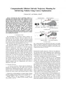
During the construction of the sequence of states in time in the PMP algorithm uses this metric to find the future vehicle state (child node) nearest to the lane goal (Figure 6). The future vehicle states are resultant from discrete commands (acceleration and steering rate) applied to a vehicle model (bicycle model). The speed goal is given by the minimum between the maximum system speed, the road speed limit and the driver preferred speed. The PMP searches to minimize the distance to these two goals. If a future vehicle state (child node) is saturated (steering or acceleration outside of the predefined limits), or is in a collision state, it is marked as a dead end and will not be used in the trajectory. B. Quintic Polynomial Planner In this algorithm is used a mathematical function that provides a geometric modelling (polynomial) of the vehicle trajectory that responds to the realistic demands of the manoeuvre to be performed. The advantage of this approach compared to the simplified PMP is that it is faster to run, however a pure geometric approach can lead to trajectories that cannot be achieved by the vehicle. To eliminate these wrong trajectories, dynamic constraints need to be added to the polynomial. To model a geometric path during a lane change, literature show often approaches using 5th degree polynomials [13][14][15]. By choosing a 5th degree (quintic) polynomial, third degree behaviour is assured for the longitudinal and lateral accelerations. A function of third degree is the minimum degree that can ensure realistic behaviour of the two acceleration components. So, the position of the vehicle must follow a function of 5th degree in the longitudinal X and lateral Y directions. The following figure shows an example of a typical lane change relative to a system of axes of reference [X, Y]. Y
r B r S
Y
X A
Fig. 7 Shortest Dubins path from point to line
This method provides the optimal path Y, connecting a point S (position and orientation) and a line L passing through the points A and B. The path consists of arcs tangentially connected by a point or a single line segment depending on the distance between the point S and the line, and the vehicle maximum turning radius at a given speed.
Fig. 8 Example of a lane change
X(t) and Y(t) will have the following formulas function of time t: X (t ) = A5t 5 + A4 t 4 + A3t 3 + A2 t 2 + A1t + A0
Y (t ) = B5 t 5 + B4 t 4 + B3t 3 + B2 t 2 + B1t + B0 The equation coefficients (A’s and B’s) are determined by specifying dynamic constraints (boundary conditions) for the
lateral and longitudinal values of the position, velocity and acceleration. See Table I. TABLE I BOUNDARY CONDITIONS ON THE LANE CHANGE TRAJECTORY Position
X (0) = 0
Initial
Y (0) = 0 Speed
inria-00533487, version 1 - 6 Nov 2010
Acceleration
X& (0) = Vinitial Y& (0) = 0
X&& (0) = 0 Y&&(0) = 0
Final X ( ∆T ) = X final Y ( ∆T ) = Y final X& ( ∆T ) = V
initial
Y& ( ∆T ) = 0
X&& (∆T ) = 0 Y&&(∆T ) = 0
The Xfinal and Yfinal are the position at the end of the lane change trajectory, ∆T is the duration of the lane change and Vinitial is the initial vehicle speed. To simplify the determination of the coefficients the vehicle speed is considered constant along the lane change trajectory and the initial and final acceleration are considered to be zero. After the geometric model coefficients are determined, X(t) and Y(t) are calculated. These points are calculated in a way that they are spaced of, at the most, half of the length of the vehicle to ensure that there is no free space between two consecutive states. This will be useful for the collision checking verification to ensure that there are no collisions between consecutive vehicle states in the trajectory. This calculated points are then added to the trajectory until the maximum number of trajectory elements is reached, the lane centre (goal) is reached or a collision is detected with an obstacle or with the road margins (e.g. end of visible lane). If the lane centre is reached and the trajectory is not full then the remaining trajectory elements are filled in with existing lane centre points. The collision checking is performed while filling in the trajectory with the determined points. A trapezoidal speed profile is attributed to the trajectory taking into account the vehicle limits in terms of lateral and longitudinal acceleration, maximum allowed speed and the possible found collision. A timestamp is then attributed the each trajectory element. V. CONTROL A typical motion control problem is the trajectory tracking, which is concerned with the design of control laws that force a vehicle to reach and follow a time parameterized reference (i.e., a geometric path with an associated timing law). According to the designed control laws, control commands are calculated based on: • the vehicle state estimation (Data Fusion); • the trajectory to be tracked, that is the best ranked trajectory according to the driving strategy (Co-Pilot); • the automation level (MSU); • direct driver controls (Driver). This command, that takes into account the vehicle physical limits (e.g. in terms of vehicle stability), is transmitted to the execution layer (vehicle actuators) composed of two components:
•
longitudinal: acceleration (engine torque or pedal braking depending on the component signal); • lateral: steering angle (or torque). A straightforward idea consisting of decoupling the longitudinal dynamics and lateral dynamics, under some simplification hypothesis, can lead to a substantial simplification of the controller synthesis phase. Indeed, with these hypotheses, the vehicle model can be divided into two linear sub-models, longitudinal and lateral, each of which is controlled by a separate control organ, engine torque and pedal braking to control the longitudinal dynamics and the steering angle to control the lateral dynamics. In this case linear robust controller synthesis techniques can be used. To compute the vehicle actions in order to keep the vehicle close to the planned trajectories, the displacement between the estimated current vehicle state (vehicle position in time) and the trajectory point to be tracked it is determined. This displacement provides the relative error between “where we are” and “where we wanted to be” for a given moment in time. Adequate control laws try to minimize this error and bring the vehicle state close to the desired one. The produced controller actions are constrained in magnitude and rate of change before being transmitted to the actuators. VI. EXPERIMENTAL RESULTS The trajectory planning algorithms described in paragraph IV were validated in the HAVEit Joint System simulation environment and in the FASCar demonstrator vehicle. The following use cases have been addressed during the experiments: lane keeping; stop behind front vehicle and adaptive cruise control (ACC); lane change and overtaking; emergency braking. The following figures and results were obtained while performing a highway scenario with three lanes and an obstacle present in the middle lane.
Fig. 9 Trajectories in the HAVEit Joint System Framework: Simplified PMP (left) and Quintic polynomial (right)
The following table shows a brief comparison of the two implemented trajectory planning algorithms. The number of obstacles influences the collision checking computation time and therefore the total execution time of the trajectory planning algorithm.
TABLE II TRAJECTORY PLANNERS COMPARISON Trajectory Planner Simplified PMP
Execution Time 250 ms
Quintic polynomial
16 ms
Advantages
REFERENCES [1] Disadvantages
Flexible; Accounts for the real time constraint of dynamic cluttered environments.
Complex; Search metric difficult to choose; Time consuming;
Fast; Analytical expressions; Realistic behaviour.
Inefficient for cluttered environments.
[2]
[3]
inria-00533487, version 1 - 6 Nov 2010
[4]
VII. FURTHER DEVELOPMENTS & PERSPECTIVES Within the HAVEit project, we plan to improve the polynomial trajectory planner by ensuring a smooth acceleration profile using a sigmoid shaped (S-curve) speed profile instead of a trapezoidal one. We will optimize the collision checking algorithm to reduce the computation time. In other future developments we would like to extend the use of the trajectory planning algorithms to urban like driving areas: complex structured (e.g. intersections, roundabouts) and unstructured (e.g parking lots) environments, interaction with a highly dynamic environments and sophisticated behaviors of surrounding obstacles (e.g. pedestrians). Also we would like to deal with different and augmented traffic rules, like traffic lights [16] and traffic signs (STOP and give way signs), and with other road markings like pedestrians crossroads, that are not contained in highway scenarios. These perspectives match partially the scope of the new French project Automatisation Basse Vitesse (ABV): Low Speed Automation. VIII. CONCLUSIONS In this paper, we addressed the problem of highly automated driving through the development of a co-pilot system. The system described here consists of two trajectory planning algorithms that were adapted in order to fit with the HAVEit project specifications where we focus on high speed driving on highways. The algorithms were integrated into the SMPLab simulator and validated using HAVEit’s FASCar research vehicle. Both approaches were tested in real conditions with different use-cases. The quintic polynomials based technique revealed more interesting performance in terms of time computations and trajectory stabilities. However, the PMP intrinsic characteristics could be more suitable for less constrained driving or for robotics-like navigation. The system will be soon exhaustively tested and validated using HAVEit’s testbeds and experimental platforms in order to validate more use cases. ACKNOWLEDGMENT Special acknowledgments here to the entire Co-pilot team in HAVEit and especially to our former colleague Rodrigo Benenson who developed the first PMP algorithm implementation.
[5]
[6]
[7]
[8]
[9]
[10]
[11]
[12] [13]
[14]
[15]
[16]
E. D. Dickmanns, and A. Zapp, “Autonomous high speed road vehicle guidance by computer vision”, 10. Triennial World Congress of the International Federation of Automatic Control. Volume IV; Munich (FRG); 27-31 July 1987. pp. 221-226. 1988. M Maurer, R. Behringer, D. Dickmanns, Th. Hildebrandt, F. Thomanek, J. Schiehlen, and E. D. Dickmanns, “VaMoRs-P: an advanced platform for visual autonomous road vehicle guidance”, Proc. SPIE, Mobile Robot Systems II, Volume 2352, 239,1995. Ch. Thorpe, M. Hebert, T. Kanade, and S. Shafer, "Vision and navigation for the Carnegie-Mellon Navlab", IEEE Transactions on Pattern Analysis and Machine Intelligence, Vol. 10, No. 3, May, 1988, pp. 362 - 373. M. Bertozzi , A. Broggi , G. Conte , A. Fascioli , R. Fascioli, “Obstacle and Lane Detection on the ARGO Autonomous Vehicle”, in Proc. of IEEE Intelligent Transportation Systems Conf.erence, 1997. F. Flemisch, F. Nashashibi, S. Glaser, N. Rauch et al., “Towards Highly Automated Driving: Intermediate report on the HAVEit-Joint System”, in the Proceedings of the 3rd European Transport Research Arena Conference (TRA 2010), 7-10 June, Brussels, Belgium. N. Rauch, A. Kaussner, H.-P. Krüger, S. Boverie, and F. Flemisch, “The importance of driver state assessment within highly automated vehicles”, presented at the 16th ITS World Congress, Stockholm, Sweden, 21.-25. September 2009. B. Vanholme, S. Glaser, S. Mammar, and D. Gruyer, “Manoeuvre based trajectory planning for highly autonomous vehicles on real road with traffic”, In Proceedings of ECC’09, Budapest, Hungary, 23-26 August 2009. C. Löper, and F. Flemisch, “Ein Baustein für hochautomatisiertes Fahren: Kooperative, manöverbasierte Automation in den Projekten H-Mode und HAVEit.”, In: Stiller, Christoph; Maurer, Markus (Hg.): 6. Workshop Fahrerassistenzsysteme. Karlsruhe: Freundeskreis Messund Regelungstechnik Karlsruhe e.V., S. 136-146, 2009. S. Petti, “Safe navigation within dynamic environments: a partial motion planning approach”, Ph.D. dissertation, École des Mines de Paris, 2007. T. Fraichard, “A short paper about motion safety”, in Proceedings of the IEEE International Conference on Robotics and Automation, 2007. R. Benenson, T. Fraichard, and M. Parent, "Achievable safety of driverless ground vehicles", in Proceedings of the IEEE International Conference on Control, Automation, Robotics and Vision, 2008. http://hal.inria.fr/inria-00294750. R. Benenson: “Perception for driverless vehicles: design and implementation”, Ph.D. dissertation, École des Mines de Paris, 2008. S. Ammoun, and F. Nashashibi, “Design and efficiency measurement of cooperative driver assistance system based on wireless communication devices”, in Transportation Research Part C: Emerging Technologies, February 2010, doi:10.1016/j.trc.2010.02.004. I. Papadimitriou, and M. Tomizuka, "Fast lane changing computations using polynomials", American Control Conference, 4-6 June 2003. T. Shamir: "How should an autonomous vehicle overtake a slower moving vehicle: design and analysis of an optimal trajectory", IEEE Transactions on Automatic Control, April 2004. R. de Charette, F. Nashashibi, “Traffic Light Recognition using Image Processing Compared to Learning Processes”, in the Proceedings of 2009 IEEE/RSJ International Conference on Intelligent Robots and Systems. St. Louis, USA, 11 – 15 Oct., 2009.