Real-Time Image Restoration with an Artificial Neural Network Gerald Krell, Andreas Herzog and Bernd Michaelis Otto-von-Guericke University Magdeburg, Institute for Measurement and Electronics PO Box 4120, D-39016 Magdeburg, Germany Telephone ++49-391-6714657, Fax ++49-391-5616358, E-mail
[email protected]
Abstract. We present a neural network that can be applied to image correction in a preprocessing unit. Blur, geometric distortion and unequal brightness distribution are typical for many scanning techniques and can lead to difficulties during further processing of an image. These and other effects of image degradation which frequently appear spacevariant can be considered simultaneously by this approach. In order to calibrate the correcting system the weights of a neural network are trained. Using suitable training patterns and an appropriate optimization criterion for the degraded images, in the result the dimensioned network represents a space-variant filter with a behavior similar to the well-known Wiener filter. The restoration result can be easily altered by the scheme of the learning data generation. Theoretical considerations and examples for 1-D, 2-D and 3-D implementations in soft- and hardware are given.
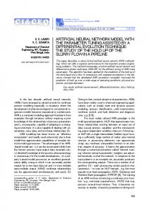
1. Introduction When operating with image signals, irregularities of the scanning system can lead to difficulties during further processing of an image such as segmentation and classification [6,7] and must therefore often be corrected. At the output of an imager array undesired effects are grey value b perceptible. As an example the scan of a regular grating by a CCD line camera in Fig. 1 demonstrates blur effects, an unequal brightness distribution and noise superposition. The geometric distortion of the lens leads to incorrect edge positions. As shown in [6], the imaging parameters are strongly space-variant and at the borders non-symmetric pulse responses are to be expected. pix el index j This kind of problems appears in the 2-D case (matrix camera) Fig. 1: Typical output of a CCD line imager for the in an analogous manner and is also typical for other scanning demonstration of frequent imaging errors techniques. As an example, in the three-dimensional confocal laser scanning microscopy [11] the direction-dependent pulse response leads to a lower bandwidth in z direction compared to x and y directions. Scaling differences between the coordinates are an additional problem. Further processing of the binary image without prior restoration would cause shape errors. The restoration of images with the mentioned degradation is a classical problem in many respects [3,5 etc.]. However, in many conventional restoration approaches knowledge about the pulse response of the degrading system, the PSF (Point Spread Function), is presupposed. A certain amount of noise is superimposed on the image as well, which is magnified by usual inverse filtering. Sophisticated restoration techniques are developed to reduce this effect [3]. Unfortunately, these methods often require a lot of effort for the design of the correcting system (transformations, statistical approaches). Moreover, operating with space-variant systems is sparsely described in the literature and the geometric distortions as well as an unequal brightness distribution (shading) must often be taken into account simultaneously. A combined solution for these problems by training the weights in a neural layer with usual learning algorithms or estimation by simple calculations, as described in the following, is an alternative. j
2. The Correcting ANN Information processing by Artificial Neural Networks (ANN) has recently become more important [8,12 etc.] and thorough investigations of biological prototypes exist [11]. One important application is the processing of visual data. In this paper, the application of ANN to the correction of optical and electrical irregularities of scanners in image processing systems is described. Some simple applications to linear space-invariant systems are already given by [9,13 etc.]. The basic ideas are extended for space-variant parameters and real-time problems. Fig. 2a illustrates the proposed general system. An ANN is inserted into the signal flow between the output of the imager array and following higher order image processing to provide a pre-processing restoration. For the restoration procedure a simple neural model can be assumed (2-D example Fig. 2b). Due to the properties of common sensor arrays (e. g.
Proc. of the International Conference on Neural Networks (ICNN '96), Washington, 03.06.-06.06.1996, pp. 1552-1557
1
CCD) a linear behavior can often be presupposed. However, normally there are small differences between the pixel ü must be defined. This elements in sensitivity and offset. If there is a remarkable offset in intensity, the bias element Θ i ,j way a locally varying offset correction can be performed by the proposed network. (a)
(b) b i − 1, j +1 b i −1 , j b i −1 , j −1
b i , j +1 oü i , j
b i,j b i , j −1
Θü i , j
b i +1 , j + 1 b i +1 , j
b i + 1, j −1
im ag e plan e
re s tau ration
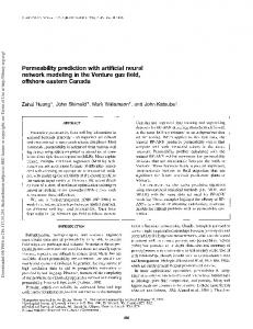
Fig. 2: System for image restoration with an Artificial Neural Network (ANN) (a) and one restoring neuron (b) In most cases image restoration should be applicable to any gray-level image. Then, a linear neuron model must be used and a single-layer network meets the requirements. According to results of linear systems theory, when suitable test patterns are used [9] to estimate the weights for the correcting layer, the expected gray-level output is achieved for all (gray-level) input patterns. In the case of binary image processing non-linear transfer functions are preferable under certain circumstances. Forming an array of restoring neurons to a single-layer neural network results in the correcting spatial filter as shown in Fig. 3a. For clarity, the principle of operation is illustrated only in one dimension without bias elements. The signals b j are the output of the image sensor that shall be corrected. The restored image oü j results after processing by the neural network. The w j ,i are weights in the correcting layer. In Fig. 3a, the output δ
oü j =
∑w
j ,i b j+ i
,
(1)
i =− δ
where locally limited interconnections are presupposed (±δ) to reduce the computational load. Conventional simulation techniques are too slow for on-line purposes (video clock rate). Usual sensor arrays have a sequential output. Therefore, pipeline processors mainly consisting of a multiplier accumulator array and representing transversal filters appear useful for modeling layers of a neural network in image processing systems [2,14]. b
b j- δ
(a)
. . .
. . .
w
b
o j+ δ
j,- δ
w j, -1
w j,0 w
b
z -1
...
w j, δ
. . .
j,i
z -1 w j, i
j+i
... w j,0
j+ δ
. . .
(c) Training of the AN N for the adaptatio n of the correc ting s ystem
w j, δ
. . .
oj
j-1
b
j+ i
. . . o
j- δ
b
j
. . .
. . .
. . .
(b )
b
j-1
o bj
z w
. . . o
j+ i
-1
b j-1
j+ δ
...
z w
j,-1
-1
b j- δ
j,- δ
oj ...
...
once or until a change of im aging conditions
R ec all of the AN N for the restauration proc ess implem ented on pipeline proc essor
on line
...
Fig. 3: Implementation of the correcting network: (a) single-layer neural network; (b) basic structure of a pipeline processor realizing a transversal filter for simulation of given neural layer in (a); (c) Steps to on-line image restoration
Proc. of the International Conference on Neural Networks (ICNN '96), Washington, 03.06.-06.06.1996, pp. 1552-1557
2
Usual pipeline processors (for example [2]) have a double set of coefficient registers that can be updated alternately during normal operation to model space-variant neural weights without lowering the throughput. For a single layer with laterally interconnected neurons, the solution is simple (Fig. 3b). The parallel input signals b j of the neural layer are sequentially fed to the pipeline processor. Storing the neighborhood of each input in a delay line the neural outputs oü j are also produced sequentially. The pipeline processor contains a multiplier accumulator array corresponding to 2δ + 1 interconnections for each neuron. The delay of the output in the serial structure of Fig. 3b is δ clock cycles, assuming a symmetric coupling. But this assumption does not hold for correction of geometric distortion. The structure of a pipeline processor for a two-dimensional array of neurons can be derived in a corresponding manner introducing delay lines [2]. An ANN for 3-D correction can also be implemented by a hardware system. The neural inputs can be summarized in z direction by the integration of delay chains for the 3-D slices into the pipeline structure. Using a pipeline processor as given in Fig. 3b, for image restoration with an artificial neural network the scheme in Fig. 3c may be used. After determination of the weights by training the neural layer with usual simulation techniques [10] a real-time recall can be calculated by the pipeline processor.
3. Determination of Weights for the Neural Layer Representing the Restoring System The adjustment of weights makes a fitting quality criterion necessary. This criterion can be varied according to the demands of the application. In image restoration the output of the correcting system should be as much equivalent to the original object intensity distribution as possible. Usually the Euclidean distance between the object (vector o ) and the restored image (vector oü ) (see Fig. 2b) should be a minimum: Q( o ) = ∑ o ν − oü ν
2
⇒ Min.
(2)
ν
Here ν is the number of different presented objects for the training of weights. Superimposed noise during the steps of image reception and processing is also considered in Eq. (2). Appropriate learning data are mandatory to allow an adaptation of the correcting system according to Fig. 4. Even if known objects are captured the object function is not given exactly because of illumination influences and positioning problems between imager and object. Therefore, after an initial estimation using a-priori knowledge about the training des pattern the desired output oü ν (target pattern) is generated which replaces the object vector o in the objective function Eq. (2). Given below is a summary of some requirements for the generation of learning patterns and for system training: • Several learning patterns with different positions are a priori know ledge necessary if isolated weights are trained (without ad es target oü → o priori knowledge). pattern generation n • For compensation of geometric distortion the edge positions must be given exactly by the test patterns. • Taking into consideration the typical spatial W H o f b oü dependence of weights, a parameter model should be (training pattern) used with the aim that the number of parameters is ad justm en t im age correction much smaller than the number of weights. This also capture reduces the quantity of training patterns. Fig. 4: Application of learning patterns to the adjustment • The quantity of learning patterns can be further of the correcting system W reduced by assuming a number of regions with spaceinvariant parameters and a limited coupling range of the neurons. • To minimize the effort for target pattern generation simple binary training patterns as gratings (1-D) or chess-like shapes (2-D) can be used. For special purposes gray shade or intentionally from learning patterns differing target patterns must be applied. In confocal 3-D images cubic test bodies are not available. But in Biology, latex beads (spheres that can be produced exactly with different diameters) are applied for cell marking that can also be used as training patterns. • Using a quadratic optimization criterion and learning patterns from images superimposed by noise directly results in a Wiener filter [3] for image correction.
Proc. of the International Conference on Neural Networks (ICNN '96), Washington, 03.06.-06.06.1996, pp. 1552-1557
3
• After a training period the network also corrects any gray-level image. The concrete behavior can be influenced by the statistical properties of the test patterns and the actual noise in the system.
4. Practical Examples Experimental results are obtained from both a line scan image sensor and from a matrix camera and initial investigations are performed with data from 3-D laser scanning (Fig. 5). These data are now compared to the theoretical predictions. (a)
x,y positioning
(b)
C C D line cam era
(c )
successiv e shift
S canning Spot
illumination training pattern
com puter with fram e grabber
object
illum ination
Laser
Beam splitter
M irror
C C D m atrix cam era
P inhole
O bjective Lens
z positioning
Photom ultiplier
intensity output R eference O bjects
Fig 5: Experimental arrangements for image capture: (a) learning data generation with CCD line camera by object shift; (b) system with CCD matrix camera; (c) image acquisition with a 3-D confocal laser scanning microscope Fig. 6 illustrates the quality criterion for the learning process. It can be considered as either a scan of a line sensor or as a single line from a 2-D image sensor. The shaded area bj A di ff oj A diff characterizes the difference between image vector b des oü j ü des and therefore the deviation of the o d e s respectiv ely and target vector o oü degraded image from the undistorted one. Analogously b de gra de d ü for restoration an area A diff between target vector and restored image has to be minimized: p ixel inde x j 2 ∑ Aü diff ⇒ Min. (3) Fig. 6: Demonstration of the quality criterion The minimization, for example, can be done with a gradient descent method typical for ANN applications [e. g. 10,12]. For a linear system the weights can be directly determined in a least mean square sense. The test pattern in the example under consideration is a periodic lattice to be reproduced by oü . In general the lattice should be scanned at several different positions to produce learning data. Fig. 7a illustrates the set of training data produced by shifting the object by equal distances. To demonstrate the abilities of the correcting neural network, blur and brightness errors were slightly emphasized by missfocussing the lens and using a non-optimal illumination, but the video signal contains a usual amount of noise.
(
(a)
(b)
250
250
200
200
150
150
)
(c)
250 200
100
100 40
50
500
1000
1500
0 2000
shift
100
40
50
40
50
20 0 0
vid eo sig nal
150
20 0 0
500
1000
1500
0 2000
20 0 0
500
1000
1500
2000
pixel index
0
Fig. 7: Numerical results for the practical example: (a) The set of original video output training patterns; (b) The corresponding target patterns; (c) The result after correction by the neural layer (recall)
Proc. of the International Conference on Neural Networks (ICNN '96), Washington, 03.06.-06.06.1996, pp. 1552-1557
4
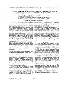
Fig. 7b shows corresponding target patterns. One layer with laterally connected processor elements (neurons) was trained using a root-mean-square criterion. The result after correction by the neural layer (recall) is presented in Fig. 7c. Because of the known edge distances of the object and corresponding edge distances in the target patterns the geometric distortion of the whole scanning system is also compensated by the calculated weights. The obvious ripple in the recall mainly results from noise amplification by inverse filtering and infringement of the sampling theorem. But in this example, the main aim was the restoration of the binary image because in measurement applications sharp edges (contours) at correct positions are often most important. To avoid strong noise amplification in other applications the learning result can be easily modified. Increasing the noise in the training data the boundary from which the frequency components are suppressed is lowered and the amplification of higher frequency components is generally reduced. So superimposing additional noise on training data the system can be optimized depending on the specific application. An alternative is the band limitation of the target patterns for the learning procedure to produce smoother recalls as output of the correcting system. Detailed results describing this method are explained in [7]. Defining space-invariant regions simplifies the generation of learning data and avoids the otherwise compulsory shift procedure for the used test pattern (lattice). The images in Fig. 8 demonstrate an example for the application of the presented approach to 2-D image restoration. The restoring ANN was trained with learning data generated from the chess board-like image (training pattern, Fig. 8a). In Fig. 8b the recall with the trained network is given. Besides the blur reduction a removal of pin cushion distortion has taken place. This is visible at the borders where due to the reduced size of the recall the original image is displayed. As mentioned above, after learning the system should correct any input provided the scanning system has not remarkably changed. Fig. 8d shows the result after application of the gray-level image (Fig. 8c) captured with the same camera and equal conditions as the training pattern to the trained network. The generalizing property of the correcting network becomes evident considering the restoration result. As mentioned above an on-line realization of image restoration is of great interest to allow a user-transparent scheme of the pre-processing. Hence, hardware implementations for 1- and 2-D applications have been undertaken. The training of the restoring network is performed by a host computer. Then, the determined neural weights are transferred to the weight memory of the pre-processing plug-in board where the space-variant correction is carried out by the pipeline processor array in real time. (a) (b) (c) (d)
Fig. 8: 2-D example for the proposed restoration: (a) training data; (b) recall with training data as input; (c) distorted gray-level image; (d) recall with (c) Fig. 9 presents an example for the restoration of 3-D images. The assumed confocal laser scanning microscope works with maximal resolution. The images are synthesized data and displayed as maximum value projections along the y axis. Fig. 9a shows an ideal sphere which is convolved by an estimated microscope PSF and superimposed by noise. The diameter of the sphere is about 20 pixel. If we apply a binarization to the image of the sphere (Fig. 9b) the shape is distorted depending on the threshold level. This problem is even more critical when measuring or recognizing irregular shapes [4]. To consider scaling errors also, we fit an ellipsoid for target data generation into the sphere. For an optimal fitting the ellipsoid is convolved with an estimated PSF. The PSF parameters are optimized during fitting in addition to the parameters for position and size. The scaling errors can be determined by the size parameters and corrected by interpolation algorithms. In the result, the target pattern can be derived from the fitting parameters. Fig. 9c shows the restored image. The differences in bandwidth between z- and x-, y- direction are equalized. As in previous examples the high frequency noise in the restored image can be lowered by decreasing the bandwidth of the target pattern. Compared to other 3-D restoration methods that are mostly iterative algorithms [1], the correcting
Proc. of the International Conference on Neural Networks (ICNN '96), Washington, 03.06.-06.06.1996, pp. 1552-1557
5
network is a 3-D FIR filter which can be better supported by hardware. (a)
(b)
(c)
(d)
Fig. 9: Application for 3-D laser scanning: (a) distorted sphere; (b) as (a), but binarized; (c) restoration of (a); (d) as (c), but binarized
5. Conclusions The investigations illustrate that using neural networks provides a relatively simple method for image restoration when the properties of the scanning system are taught to the correcting neural network during calibration. The neural network also compensates for some often unknown influences and optimizes the system in the presence of noise without any additional calculations. The inevitable compromise between enhancement of contours and noise amplification can easily be adjusted. In comparison with space-invariant [9] filters the results are significantly better. After a phase of learning, on-line processing by pipeline processors can emulate neural layers. For real-time processing, the proposed solution requires only available pipeline processors. System training during calibration is performed by software, and additional hardware is unnecessary.
Acknowledgment The authors are grateful to the Federal Institute of Neurobiology Magdeburg (Director H. Scheich) for providing the 3-D data and the general backing of the work. This work was supported by BMBF grant (01 M 3018 E/3) and DFG/BMBF grant INK15/A1.
References [1] J.-A. Conchello, E. W. Hansen: Enhanced 3-D reconstruction from confocal scanning microscope images. Applied Optics Vol. 29, No. 26, 10 September 1990, pp. 3795-3804. [2] The Digital Signal Processing Databook: Product guide INMOS. 1989. [3] R. C. Gonzalez, P. Wintz: Digital Image Processing. Addison-Wesley, 1987. [4] A. Herzog et al: Analysis of Morphological Spine Changes by Restaurated 3-Dimensional Images. Interdisciplinary Workshop and Autumn School on Neural Network, Würzburg, 12.10.-14.10. and 16.10-18.10.1995, Proc. pg. 40. [5] H. Jahn, R. Reulke: Systemtheoretische Grundlagen optoelektronischer Sensoren, Akademie Verlag, 1995. [6] Michaelis, B.; Krell, G.: Neural Networks for Image Improvement in Optoelectronic Measuring Devices. IMTC/92 , New York, 12.-14.05.1992. [7] B. Michaelis, G. Krell: Artificial Neural Networks for Image Improvement. Lecture Notes in Computer Science 719, Springer 1993, pp. 838-845. [8] C. Lau: Neural Networks. IEEE Press 1992. [9] H. Marko: Die Systemtheorie der homogenen Schichten. Kybernetik 5, pp. 221-240 (1969). [10] NeuralWorks Professional II/PLUS and Neural Works Explorer: Reference Guide. Pittsburgh: NeuralWare Inc., 1991. [11] J. B. Pawley (editor): Handbook of Biological Confocal Microscopy. Plenum Press, New York, revised edition 1989. [12] E. Sanchez Sinencia, C. Law: Artificial Neural Networks. IEEE Press 1992. [13] W. v. Seelen: Informationsverarbeitung in homogenen Netzen von Neuronenmodellen. Dissertation Technische Hochschule Hannover 1967. [14] N. Storey; R. C. Staunton: An Adaptive Pipeline Processor for real-time image processing, Proc. SPIE, Paper No. 1197-23, November 1989.
Proc. of the International Conference on Neural Networks (ICNN '96), Washington, 03.06.-06.06.1996, pp. 1552-1557
6