754
IEEE TRANSACTIONS ON IMAGE PROCESSING, VOL. 15, NO. 3, MARCH 2006
Real-Time Processing and Compression of DNA Microarray Images Shadrokh Samavi, Shahram Shirani, Senior Member, IEEE, and Nader Karimi
Abstract—In this paper, we present a pipeline architecture specifically designed to process and compress DNA microarray images. Many of the pixilated image generation methods produce one row of the image at a time. This property is fully exploited by the proposed pipeline that takes in one row of the produced image at each clock pulse and performs the necessary image processing steps on it. This will remove the present need for sluggish software routines that are considered a major bottleneck in the microarray technology. Moreover, two different structures are proposed for compressing DNA microarray images. The proposed architecture is proved to be highly modular, scalable, and suited for a standard cell VLSI implementation. Index Terms—DNA microarray images, hardware architecture, image processing, pipeline.
I. INTRODUCTION
I
N THE past few years, molecular genetics has received a great deal of attention. Recent discoveries and new techniques have made it possible to characterize diseases and show the effect of drugs on microorganisms. DNA is the basic hereditary material in all cells and contains all the information necessary to make proteins. DNA is a linear polymer made up of nucleotide units, characterized by four types of bases: adenine (A), thymine (T), guanine (G), and cytosine (C). In normal DNA, the bases form pairs: A to T and G to C. This is called complementarity and contributes to determine the DNA shape. Fig. 1 shows the double helix structure of a typical DNA. The DNA structure can be divided into two helices (single strands) and then recomposed with a process called hybridization. Only complementary single strands can hybridize together. Genes are encoded in the sequence of chemicals that make up DNA. When a particular gene codifies a protein, it is said to express into the protein [1]. The number of experiments that are required to fully characterize an organism by means of gene expressions is huge. Yeast alone contains 6116 genes and it requires more than 700 000 gene expressions to characterize it [2]. Traditional methods of laboratory experiments required years of investigation to characterize a disease. DNA microarray analysis is a recently developed technique, which allows the study and classification
Manuscript received December 12, 2004; revised January 10, 2005. This work was supported in part by Micronet and in part by McMaster University. The associate editor coordinating the review of this manuscript and approving it for publication was Dr. Christophe Molina. S. Samavi and N. Karimi are with the Department of Electrical and Computer Engineering, Isfahan University of Technology, Isfahan, Iran (e-mail:
[email protected]). S. Shirani is with the Department of Electrical and Computer Engineering, McMaster University, Hamilton, ON L8S 4K1, Canada (e-mail:
[email protected]). Digital Object Identifier 10.1109/TIP.2005.860618
Fig. 1. Structure of a DNA.
of genes in a much shorter time than ever before. This technology, which is briefly explained here, allows compression of thousands of DNA nucleotide sequences on a single microscope glass. A leading use of DNA microarrays is in determining which subset of a cell’s genes are expressed, or are actively making proteins, under certain conditions, such as exposure to a drug, toxic material, or malignancy. The substrate of a microarray consists of a piece of glass, or sometimes a silicon chip, similar to a microscope slide. Onto this substrate, thousands of patches of single-stranded DNA are fixed which are called probes. A typical microarray is a 2 4-cm membrane or a microscope glass slide with a probe diameter of 75–100 m and a 150- m distance between probes. The location and sequence of each patch of DNA are known. Microarray technology is based on the ability of complementary base pairing of the nucleic acids. “Probe” DNA strands are spotted onto the chip. Probes are single strands with known sequences and are used as a template to identify the unknown agents. “Target” DNA mixture is then washed onto the chip to allow base pairing that means only highly complementary sequences will remain bound to their pairs. Single strands in
1057-7149/$20.00 © 2006 IEEE
SAMAVI et al.: REAL-TIME PROCESSING AND COMPRESSION
Fig. 2.
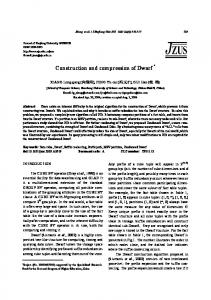
Typical unprocessed microarray image.
the target mixture may come, for instance, from healthy and cancerous cells. The goal could be to identify genes that are responsible for malignancy [3]. The target DNA mixture is labeled with different fluorescent dyes to distinguish between DNA originating from different experimental conditions. For instance, DNA from blood cancer cells may be labeled with red fluorescing dye and those from normal blood cells with green fluorescing dye. These dyes are detected using laser excitation. Fluorescent intensity corresponding to each dye is recorded separately for each spot on the array. These images are superimposed for each spot to arrive at the actual gene expression pattern for the cancerous blood cells. The array of spots fluorescing purely red represent genes expressed only under cancerous conditions, while those that are pure green correspond to genes expressed solely under normal conditions. Genes that are expressed under both conditions will appear as spots of varying degrees of yellow. Fig. 2 shows a typical gray scale microarray image. The main bottleneck in the application of DNA microarrays is now the time-consuming analysis of the spots in the obtained image. This is currently done mainly by software systems. These software packages vary depending on the manufacturer of the microarray chip as well as the specific application of the chip. The time required for the analysis could range from several minutes to hours, depending on the required image quality and the proficiency of the operators. When there is a race to find means for identifying new deadly and highly contagious viruses every second is crucial. A well-known software package for microarray image analysis is ScanAlyze, which requires the operator to take 14 steps [4], many of which have to be repeated several times. Many commercial vendors have come up with software packages, which eliminate some of the manual steps of ScanAlyze. Hardware implementation of microarray image analysis seems to be an attractive alternative to the software schemes as hardware is inherently faster than software. One of the main research works that has focused on hardware implementation of microarray image analysis is by Arena and his coworkers [5], [6]. They use cellular neural networks (CNNs) and a mixed signal dedicated CPU called
755
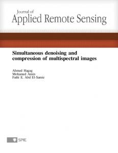
“CNN universal machine.” Their proposed hardware requires parallel inputs from the pixels of the image and eventually outputs the processed image in a parallel format. Therefore, there are serious limitations on the size of the image that can be processed due to a limited number of I/O ports that a VLSI chip can have [7]. Hence, the image has to be subdivided into “tiles” which in turn requires operator intervention. In this paper, new architectures for close to real-time processing and compression of DNA chip images are proposed. The main advantage of our processing architecture is the fact that large DNA images could be processed in less than a millisecond. As mentioned before, any reduction in overall processing time is multiplied by large number of processes that are required in a complete gene characterization. Our approach, due to the time overlap capabilities of the pipeline structures, makes the whole process a semi parallel one [8]. Therefore, near to real-time performance can be achieved for a processing phase which for most cases is now very sluggish [9], [10]. Moreover, we propose two architectures for the compression of microarray images. Microarray images are usually massive in size. A typical 100 000spot microarray may easily end up as a 30-Mbyte image. Since some applications require these images to be transmitted, the need for fast microarray image compression is growing. This paper is organized in the following manner. Section II briefly describes the required steps in processing of DNA microarray images. In Section III, details of the proposed image processing hardware are discussed. The compression of DNA microarray images is discussed in Section IV where different structures for this purpose are offered. Section V is dedicated to analysis of the results of simulation and implementation of the pipeline. Hardware requirements of the suggested architecture are discussed in Section VI. Concluding remarks are presented in Section VII. II. IMAGE PROCESSING STEPS A DNA microarray image initially has four types of pixels: background, green, red and yellow. This colored image is first converted into two gray scale images. There will be one gray scale image corresponding to the red component and one corresponding to the green component of the color image. The yellow pixels will be present in both images [11]. A number of image processing steps will be performed on each image. Background noise has to be eliminated. Small spots as well as spots that are not in their presumed locations should be removed. Fig. 3 shows the processing steps that the image processing part of the pipeline performs on gray level images. In the following, some details of each processing step are explained. a) Noise elimination is performed by a thresholding process. When the microarray is illuminated by a light source, the hybridized DNA collections are the main regions that emit light, but other parts of the glass slide also scatter and emit some background light. This occurs due to binding of fluorescent dyes to the glass slide. Different methods of dealing with this background intensity are suggested in the literature [10]. We used the “constant background” method. In this method, it is assumed that a constant background exists throughout the image. This constant
756
IEEE TRANSACTIONS ON IMAGE PROCESSING, VOL. 15, NO. 3, MARCH 2006
of “erosion” and “dilation” remove these spots. These algorithms are briefly explained in the followings. (corresponding to the Erosion: For sets and in pixels in objects), the erosion of by , denoted and is defined as
where
is the translation of a set and is defined as
by point
Thus, the erosion of by is the set of all the points such that , translated by , is contained inside . One of the main applications of erosion is elimination of irrelevant details from a binary image [12]. , the Dilation: Assuming that and are sets in is defined as dilation of by , denoted by
where Fig. 3.
is the reflection of set
and is defined as
Block diagram of the image processing part of the pipeline.
background intensity depends on the technology and material that are used in manufacturing of the microarray chip. The background intensity value can be obtained experimentally by placing “negative control spots.” These are spots that do not hybridize with target DNA samples and their intensity is an indication of the background noise. We use this background intensity as a threshold value. Applying a threshold value to all pixels of the image would remove most of the background noise. Exceptions are high intensity spikes that have to be dealt with by other means. The thresholding process also eliminates spots with low intensity levels, which are mainly spots with lower degrees of hybridization. These spots are mainly due to anomalies in microarray fabrication. Therefore, elimination of low intensity spots is a desirable byproduct of thresholding. Thresholding generates a binary image called binary map, which is 1 at pixel locations above the threshold and 0 otherwise. As shown in Fig. 3, the grid placement, erosion, and dilation steps are performed on this binary map. b) Dislocated spots are created by defects in the microarray or by preillumination processes. In the matrix structure of a microarray, there are prescribed locations in which a spot is expected to exist. Spots that are not within their expected perimeters should be considered as anomalies and be removed. This is done by applying a grid on the binary map through an AND operation between the binary map and a predefined grid mask. Therefore, any spot that crosses a grid line is set to zero. c) Small spots in the image could either be spikes of noise with above-threshold intensity levels or a small number of hybridized DNAs that are concentrated in a small area. In either case, two consecutive morphological algorithms
is commonly referred to as the structuring element. Essentially, dilation of by is the set of all disand overlap at least one placements, such that pixel. One of the simplest applications of dilation is for bridging gaps and filling small holes in an image [12]. By performing an erosion step followed by a dilation procedure on a binary map, small isolated spots are removed while regular spots will maintain their original size. The size of the structuring element will determine the size of spots that are removed. On the other hand, the shape of the structuring element determines how the edges of the spots are eroded and dilated back again. Intuitively, the size of the structuring element should be set to the average radius of the spots in the microarray image. This way, normal spots will be preserved after the erosion-dilation steps while small spots are removed. The average radius of the spots in a microarray image can be easily calculated based on the size of the spots when the array was manufactured and the resolution of the imaging system. d) Masking is basically an AND operation that is performed between the binary map (which is generated through grid placement, erosion and dilation steps) and the original DNA gray-level image. Masking of the DNA image with the binary map results in a gray-level image containing those pixels in the input DNA image with a corresponding “1” in the binary map. The image generated by masking does not have any background noise and is free of other artifacts such as misplaced or small spots. In the following section, we explain a pipelined hardware architecture that we developed for performing the above DNA image processing steps.
SAMAVI et al.: REAL-TIME PROCESSING AND COMPRESSION
Fig. 4.
757
First stage of the pipeline.
III. PIPELINE IMAGE PROCESSING ARCHITECTURE In this section, we present details of the proposed pipeline architecture. The first stage of the pipeline is shown in Fig. 4. Suppose that each row of the image has 256 pixels and each pixel has an 8-bit gray scale intensity. For the sake of illustration, it is assumed that a 32-bit data bus transfers the image from the
image acquisition circuitry to the pipeline. It, therefore, requires 64 clock pulses to bring in one row of pixels. While transferring the pixel values to the first stage of the pipeline, the threshold value is subtracted from the intensities. Hence, a binary map is generated based on the sign bits of the result of this subtraction. It will be on this map that the grid is applied and morphological algorithms are performed. Through
758
IEEE TRANSACTIONS ON IMAGE PROCESSING, VOL. 15, NO. 3, MARCH 2006
Fig. 5. (a) 2
2 2, (b) 5 2 5, and (c) 9 2 9 structuring elements.
the masking process, the binary map is finally used to assign the original gray scale value to pixels that have corresponding 1s in the map. The binary map should have 0s at the grid locations. In other words, pixels that overlap the grid lines are set to zero. This job is also done in this stage by an array of AND gates. Vertical grid lines have fixed positions in the array with a permanent “0” input, while the horizontal grid lines occur at every M row and have a width of P pixels. A simple state machine produces the necessary signaling for the horizontal grid generation. Morphological algorithms that were mentioned in the previous section require a structuring element. As explained before, the size and shape of these structuring elements have substantial effects on the quality of the final image. Fig. 5 shows three structuring elements that have been examined in this paper. Stages 2 onward of the pipeline are shown in Fig. 6, where a 5 5 structuring element is used. Stages 2–6 of the pipeline, in this case, perform the erosion algorithm and the first auxiliary stage stores the resulting binary map. The auxiliary stages are the ones that work with the falling edge of the clock pulse, unlike the regular stages of the pipeline that use the rising edge of the clock signal. To keep the diagrams simple, only the first five pixels of each row is shown in Fig. 6. For the same reason, the erosion circuitry for only one pixel is shown. Other pixels are treated in a similar manner. Stages 7–11 of Fig. 6 perform the dilation algorithm. The second auxiliary stage holds the result of this algorithm. The binary map obtained at this stage is used to mask the gray level image. This is done by performing an AND operation between the mask and the gray level image. This way, only pixels with a value of 1 in the map will maintain their gray level value and all other pixels (mainly background noise and isolated specks) will be assigned a value of zero. This mapping process is performed by stage 12 of the pipeline. IV. IMAGE COMPRESSION Microarray technology is a powerful tool for simultaneous study of the activities of thousands of genes. To study a simple microorganism, a large number of microarray images are produced. Storage of these images requires the occupation of a large memory space [13]. In a number of applications, these images should be transmitted on a wireless transmission medium. It is, therefore, essential to compress these images before they can be serially transmitted. In this section, we introduce two architectures for image compression using pipeline structures. Either of
these two structures can be added to the image processing part of the pipeline. In no random image is there a correlation between the intensity of a pixel and that of its neighbors. If the intensity of a pixel is and the intensity of its neighboring pixel (on the same row) , it is very likely that there is a small difference between is and . This phenomenon is known as spatial redundancy. Compression of still pictures is often based on this spatial redundancy. Two main categories of compression methods are lossy and lossless schemes. In lossless schemes, the restored image is identical to the original image and no loss of data occurs in the compression process [14]. Huffman coding and run length encoding (RLE) [15] are two well-known lossless compression schemes. In lossy methods, less important parts of the image, which usually lie in the details, are lost in the compression process. Schemes such as vector quantization and transform coding are among lossy compression schemes [14]. Due to the importance of the intensity level of each spot in the microarray image, it is vital to use lossless algorithms to compress them. Microarray images obtained from a specific set of equipment have a fixed matrix-like form. This means that the number of spots, the distance between them, and average spot size are known. The histogram of Fig. 7 belongs to a typical microarray image. It reveals that some of the intensity levels have high probability of occurrence while some may occur less frequently. After a microarray image is processed, as explained earlier in this paper, about 80% of its pixels have zero intensity. Therefore, using a lossless scheme, which is based on the probability distribution function of the intensity levels, seems to be a good choice. In [13], [16], and [17], different techniques have been proposed for compression of microarray images. In all of these schemes, implementations have been software based. In the following, we present two pipeline architectures, based on two different algorithms, for microarray image compression. In our synchronous pipeline architectures, at each clock pulse, only one row of the image can be compressed and get prepared for transmission. Therefore, only one-dimensional (1-D) spatial correlation among the neighboring pixels is used. Also, the number of bits in a compressed line of a microarray image is a function of intensity of the pixels of that line. This means that the number of pulses required to serially transmit a compressed line of the image is variable. We, therefore, designed the pipeline in a way to perform compression and serial transmission irrespective of the intensity distribution of the pixels. Due to these hardware restrictions, our architecture achieves a lower compression ratio compared to compression schemes that employ the two-dimensional (2-D) correlation (e.g., JPEG-LS, or the methods proposed in [16] and [17]). Fig. 8 shows one implementation of the image compression stage of the pipeline. We process the pixels of the image in a raster scan order. This scheme uses a predictive coding algorithm to produce a residual sequence for each raster scan. The following equation shows how the residual sequence is generated: (1)
SAMAVI et al.: REAL-TIME PROCESSING AND COMPRESSION
Fig. 6.
759
Image processing stages of the pipeline using a 5
Fig. 7.
2 5 structuring element.
Histogram of a typical microarray image.
where and are the intensity values of two adjacent pixels. It has been noticed that it is only at the edges of the spots that the difference between two neighboring pixels is relatively high. In all other cases, when traversing inside spots or on background pixels, the mentioned difference is very small. A large pool of microarray images has been statistically analyzed in [17], and it was concluded that approximately 90% of the produced residuals were zero. It was, therefore, decided to perform Huffman coding on these generally small-magnitude
residual sequences, and a Huffman code was designed for the residues. At each clock pulse in Fig. 8, one of the C1, C2, , C128 timing signals is activated and three adjacent pixels are sent to two subractors. A Huffman code has been extracted for these residuals. The longest Huffman code was found to be 14 bits long. Two look-up tables (LUTs) have been dedicated to store these codes. When the Huffman code is fetched from a LUT it is sent to the next stage of the pipeline where it
760
IEEE TRANSACTIONS ON IMAGE PROCESSING, VOL. 15, NO. 3, MARCH 2006
Fig. 8. Implementation of Huffman coding based on differential coding algorithm.
will be serially transmitted. Since the prediction residue is 9 bits long, the number of entries of each LUT is 512. Each entry of the table has 18 bits, where 14 bits belong to the Huffman code. A Huffman code is a variable length code (VLC). It means that in most cases the 14-bit space will not be completely filled. The number of bits of each Huffman code is stored in a 4-bit space along side of the code. Fig. 9 shows the pipeline stage for serially transmitting the generated Huffman codes. Serially transmitting a variable length code with a pipeline structure, where all timings are predefined, is a difficult task. Shorter Huffman codes take fewer clock pulses to be serially transmitted. Furthermore, the length of a code is not known until it is generated. A code length could be anything between 1 to 14 bits long. The transmission stage has to accommodate the worst-case
situation. Therefore, one 14-bit shift unit is available for every residual code. The corresponding Huffman codes are stored in these shift units. The length of each code is loaded to a count unit. This count unit determines the number of pulses that is needed to shift out the Huffman code onto the serial output bus. In Fig. 9, only two count and shift units of a row of these units are shown. Our second compression architecture is based on RLE. RLE is an efficient compression method for the processed microarray images since there are a large number of consecutive zero intensity pixels. In its original form, RLE looks for a sequence of pixels with same intensity levels. It assigns two bytes for that sequence; one byte for the intensity level and one byte for the number of pixels in the sequence. If neighboring pixels have different intensity values, then this schemes fails to compress the
SAMAVI et al.: REAL-TIME PROCESSING AND COMPRESSION
761
number of generated blocks is not known in advance. The content of this last counter is used to generate correct number of pulses necessary to transmit the compressed data. In order to distinguish between a zero-intensity pixel and a nonzero pixel, C1 to C256 timing signals are used. With the arrival of each timing-signal, values of two adjacent pixels are tested for being zero. If both pixels are zero, the content of counter (B) is incremented. In the case that either of the pixels is nonzero, it indicates the end of a sequence. Hence, a 9-bit block is then generated. The worst-case scenario occurs when we need to compress a row of the image that passes through the center of a row of spots. In this case, there are minimum background pixels with zero intensity and maximum gray-level pixels belonging to the spots. Therefore, in the worst case, bits are generated. Simulation results show that is 1170 bits (corresponding to 130 blocks each 9 bits). In other situations, the number of blocks would be less. The pipeline has to support the worst-case scenario. Therefore, a row of 9-bit registers is available to hold the generated values. In order to serially transmit these blocks, the number of 9-bit blocks should be known. This number is generated and bit counter (C). The number of blocks kept in a is multiplied by 9 to come up with the number of bits that are to be serially transmitted. This number is stored in a bit count unit. The compressed line of the image is then loaded into a shift unit. The shift unit and the single count unit are considered as a separate stage of the pipeline. The content of the shift unit goes on a serial transmission line. When the transmission is terminated, the connection to the line is severed through a tri-state connection. V. SIMULATION AND IMPLEMENTATION RESULTS In this section, we present the simulation and implementation results of proposed processing and compression architectures. A. Processing Architecture
Fig. 9. Final stage of the pipeline responsible for serial transmission of the image.
information. This is because it will assign two bytes for every pixel. We came up with a scheme that we call pseudo RLE. In this scheme, we compress the information in 9-bit blocks. If the MSB of the block is zero, then the remaining 8 bits represent the length of sequence of adjacent zero-intensity pixels. If the MSB of the block is 1, then the remaining 8 bits represent the intensity value of a single pixel. Fig. 10 shows two stages of the pipeline dedicated to pseudo-RLE compression and its serial transmission hardware. Three counters have been used in these stages. The first counter (A) is responsible for generating C1, C2, , C256 timing signals. Another counter (B) is to count the number of consecutive pixels with zero intensity. The third counter (C) keeps track of the number of 9-bit blocks of data that are generated during the compression procedure. Obviously, the
The proposed processing architecture was implemented for 2 2, 5 5, and 9 9 structuring elements. Fig. 11(a) shows a typical microarray image. Background noise and specks as well as DNA probes are present in that image. Probes (i.e., spots) in that image have an average radius of six pixels. The results of processing this image with the proposed architecture are shown in Fig. 11(b)–(c). Fig. 11(b) shows the output image of the process when a 2 2 structuring element is used. Some of the small spots that were larger than 2 pixels in diameter remain in the output image. The use of a 9 9 structuring element caused elimination of some of the probe spots which were smaller than the structuring element. This situation is shown in Fig. 11(d). The structuring element of choice turned out to be a 5 5. This was expected since, as mentioned in Section II, an structuring element works best when is close to the average radius of spots. The results for the 5 5 case is shown in Fig. 11(c), where background noise and small spots were removed but no above-threshold probe spot was eliminated. In all images of Fig. 11, the grayscale values of pixels are subtracted from 255. This is not a part of the hardware operations and is merely done for illustration of the results.
762
IEEE TRANSACTIONS ON IMAGE PROCESSING, VOL. 15, NO. 3, MARCH 2006
Fig. 10.
Implementation of the suggested pseudo RLE algorithm.
The useful biological information of the microarray image is embedded in the intensity and location of the hybridized spots. During the image processing steps of the suggested architecture intensities of the spot pixels remained intact. The only concern can be loss of a small number of spot pixels due to the morphological operations (i.e., erosion and dilation). Fig. 12 shows a typical binary map after the morphological operations have been performed. In Fig. 12, the eliminated pixels are shown in gray.
We performed a statistical analysis on 21 images. The average intensity of the spots in the processed images turns out to be 2.238 lower than the average of intensity of spot in the input images due to the lost pixels. This is lower than the array-to-array structuring element, it is posvariability [18]. Using an sible to lose pixels on the edges of the spot in a region which is pixels wide. Hence, using a 5 5 structuring element, one or two pixels could vanish from the edges. Depending on the
SAMAVI et al.: REAL-TIME PROCESSING AND COMPRESSION
763
2
Fig. 11. (a) Unprocessed microarray image. (b) Output image of the process when a 2 2 structuring element is used. (c) Output image of the process when a 5 5 structuring element is used. (d) Output image of the process when a 9 9 structuring element is used.
2
Fig. 12.
2
Example of a bit map after performing the morphological operations.
shape of the boundary and the geometry of the structuring element, it is possible that an eroded pixel is not recovered in the dilation process (there are spots that none of the boundary pixels is deleted after erosion dilation). The lost pixels are a small fraction of the original spot’s boundary pixels. Our analysis showed that the deleted pixels are distributed among the spots of the image and are not localized. Therefore, the spots’ biological information remain unharmed. The size of the architecture that is used here is only a function of the width of the input image and is independent of its length. Furthermore, the pipeline is static and does not require reconfiguration while an image is being processed. Therefore,
structural, data, and control hazards that are present in many dynamic pipeline structures are absent in our design, which adds to the reliability of this design [19]. The main bottleneck in the application of DNA microarrays is the time-consuming analysis of the obtained image. In fact, the full potential of DNA microarray technology has not been exploited in part because of difficulties in performing real time analysis of DNA images. Therefore, any progress in speeding up the analysis process or making even a part of it automatic, will result in great advances both in research and practical applications of microarray technology. Our proposed architecture, thanks to its pipeline structure, makes DNA image processing semi-parallel and real time. Therefore, the use of our pipelined architecture could impact the speed of analysis of DNA microarray images. B. Compression Architecture In this section, we discuss the results of the two compression schemes. We use pipeline speedup as a measure to compare the clock period of a pipeline that has a compression stage with a pipeline that has no such stage. When the processing of a row of the image is over, we have a row of 8-bit pixels sitting next to each other. This means for example, we have a row of 256 of 8 bits. We need to find the prediction residue between two adjacent groups of bits. Usually, groups of 8 bits are considered. We examined other group lengths, too. In different experiments we divided the mentioned
764
IEEE TRANSACTIONS ON IMAGE PROCESSING, VOL. 15, NO. 3, MARCH 2006
Fig. 13.
Effect of bit-group size on efficiency of different compression techniques.
gates, large multipliers, wide function capability, a fast carry look-ahead chain and a cascade chain. The results show that less than 21% of the available assets have been utilized for the compression and transmission stages. This implies that the processing, compression and transmission circuitry is easily fit on a reconfigurable chip; hence, custom implementation of the design would require small silicon area. VI. CIRCUIT COMPLEXITY
Fig. 14. Effect of LUT size on the speedup of the pipeline in differential Huffman scheme.
row into groups of 2 to 13 bits. The Huffman codebook for the prediction residues of these groups was computed. Fig. 13 shows the speedup of the pipeline as a function of these block sizes. The differential coding with a block size of 9 bits produces the greatest speedup. Fig. 13 also reveals that the peak speedup for pseudo-RLE occurs when 8-bit groups are used. Differential coding scheme is affected by the size of the LUT. This effect is shown in Fig. 14. It can be seen that an LUT size of 18k bits produces the largest speedup. In our pipeline architectures, at each clock pulse, only one row of the image can be compressed; therefore, only 1-D spatial correlation can be exploited. This results in a lower compression ratios compared to the schemes that employ the 2-D correlation. Our experiments show that the average compression ratio that the proposed architecture achieves is approximately 60% of that of JPEG-LS. For example for a processed microarray image the compression ratio of our proposed architecture is 1.8:1 compared to 3:1 from JPEG-LS. The suggested structures were implemented using Virtex II FPGAs from Xilinx Corporation. Table I shows the implementation results of the two compression and transmission architectures. In Table I, CLB stands for configurable logic blocks. CLBs provide the functional elements for combinatorial and synchronous logic. CLB resources include four slices and two three-state buffers. The slices are equivalent and each contains two function generators, two storage elements, arithmetic logic
In this section, hardware requirements of the proposed pipeline are discussed. The pipeline is capable of processing, pixels in every compressing, and transmitting an image with row. We first look at the requirements of the first part of the pipeline that processes the image. Suppose that the input data bus is bytes wide and a threshold value of is selected. Also, structuring element is to be implemented assume that an and an external clock with frequency is available. The first stage of the pipeline requires subtractors and ( -bit) registers where if if if if
(2)
For 8-bit gray scale pixels a threshold of 128 can easily be implemented. The most significant bit (MSB) of the intensity can be taken as the outcome of the thresholding process. Pixels with an MSB of 1 are above threshold and others are below threshold. Therefore, comparators are not needed. Furthermore, it is not necessary to save the map in a separate location since the intensity contains the map value as its MSB. As mentioned in (2), if any threshold value other than 128 is used, then an extra one bit is required to hold the corresponding binary map. clock pulses to fill out stage one of the It will take regular pipeline. Beside stage 1, there are a total of each consists of and two auxiliary stages. Stages 2 to ( -bit) registers. Stages to each has 1-bit
SAMAVI et al.: REAL-TIME PROCESSING AND COMPRESSION
765
TABLE I IMPLEMENTATION RESULTS FOR DIFFERENT COMPRESSION TECHNIQUES
TABLE II HARDWARE REQUIREMENT FOR DIFFERENTIAL HUFFMAN SCHEME
TABLE III HARDWARE REQUIREMENT FOR PSEUDO-RLE SCHEME
registers. Stage which is the final one has registers where each of the registers has bits. Each of the auxil1-bit registers. Overall, the number of one-bit iary stages has storage elements required for the image processing part of the . proposed architecture is Connecting an external clock with a frequency of 133 MHz causes the stages of the pipeline to operate with a frequency of 2.078 MHz. This is because the implemented pipeline requires 64 clock pulses to fill out its first stage. The delay of the first stage when processing an image with 256 256 pixels is 0.48 s, which determines the pipeline clock period. In general, seconds. Based on the disthe pipeline clock period is seconds for cussions of this section, it takes the whole image to be processed. Using a 5 5 structuring element; therefore, it takes 126 s of processing. This is without the compression and transmission stages connected. The cellular neural network hardware processes a 64 64 image in 7 ms [5], [6]. In this regard, our pipeline architecture shows a speed up of two orders of magnitude. We now look at the requirements of the compression and transmission stages. Suppose that H is the number of bits for the longest Huffman code. Then, Table II shows the required hardware for the compression and transmission stages of the differential Huffman algorithm. Let be the number of bits in the longest compressed line in pseudo-RLE method. Hardware assets that are required for the compression and transmission stages of this algorithm are shown in Table III. Using a 133-MHz clock and employing pseudo-RLE scheme results in a pipeline clock period of 8.8 s. In implementation was taken to be 1170 bits. This causes a of this scheme, 256 256 pixel image to go through processing, compression, and transmission in 2.25 ms.
The proposed architecture is easily expandable. If images of 512 512 pixels are to be processed, the input and output lines do not need to be increased compared to when 256 256 pixel images were processed. The width of the pipeline and the number of storage and logic elements have to increase according to the relations mentioned earlier in this section. Smaller images can be processed on a hardware that is designed for larger images. As in any hardware implementation of software routines, there is a trade off between flexibility and speed. Hardware is faster but less flexible. A hardware alternative to the proposed pipeline architecture is a parallel structure which pixel image requires hardware assets for an (I/O and required silicon area). Our architecture has complexity. The image acquisition is usually a row-by-row process [20]. Therefore, for this application, having a fully parallel architecture would not improve the processing time as compared to a pipeline structure. VII. CONCLUSION Microarray technology, which has drastically improved the gene recognition and classification routines, has been lacking a real time image analysis and compression technique. In this paper, we presented a new pipeline architecture that uses the inherent delay in generation and transmission of images. We further offered a new implementation of the differential coding for compression of microarray images. A new compression algorithm and its implementation was also presented and proved to be functional. These designs will close the time gap between the generation of a microarray image and its analysis. The proposed architecture was implemented on a number of FPGAs. The circuit complexity for a certain structuring element is only a function of one of the image dimensions and it grows linearly as the size of the image increases. Overall, the architecture proved to be scalable, modular, and versatile. REFERENCES [1] P. O. Brown and D. Botstein, “Exploring the new world of the genome with DNA microarrays,” Nature Gen., vol. 21, pp. 33–37, 1999. [2] O. Alter, P. O. Brown, and D. Botstein, “Generalized singular value decomposition for comparative analysis of genome-scale expression data sets of two different organisms,” Proc. Nat. Acad. Sci., vol. 100, no. 6, pp. 3351–3356, Mar. 2003. [3] M. K. Szczepanski et al., “Enhancement of the DNA microarray chip images,” in Proc. 14th Int. Conf. Digital Signal Processing, vol. 1, 2002, pp. 395–398. [4] D. E. Bassett, M. B. Eisen, and M. S. Boguski, “Gene expression informatics—It’s all in your mine,” Nature Gen. Suppl., vol. 21, pp. 51–55, 1999. [5] P. Arena, L. Fortuna, and L. Occhipinti, “A CNN algorithm for real time analysis of DNA microarrays,” IEEE Trans. Circuits Syst. I, Fundam. Theory Appl., vol. 49, no. 3, pp. 335–340, Mar. 2002.
766
[6] P. Arena, M. Bucolo, L. Fortuna, and L. Occhipinti, “Cellular neural networks for real-time DNA microarray analysis,” IEEE Eng. Med. Biol. Mag., vol. 21, no. 2, pp. 17–25, Mar./Apr. 2002. [7] M. L. Schmatz, “High-speed and high-density chip-to-chip interconnections: Trends and techniques,” in Proc. IEEE Conf. Electrical Performance of Electronic Packaging, 2000, pp. 23–24. [8] S. Samavi, S. Shirani, and N. Karimi, “A pipeline structure for analysis of DNA microarrays,” in Proc. IEEE Pacific Rim Conf., Aug. 2003, pp. 1012–1015. [9] C. Uehara and I. Kakadiaris, “Toward automatic analysis of DNA microarrays,” in Proc. 6th IEEE Workshop on Applications of Computer Vision, 2002, pp. 57–62. [10] R. Hirata Jr. et al., “Microarray gridding by mathematical morphology,” in Proc. XIV Brazilian Symp. Computer Graphics and Image Processing, Oct. 2001, pp. 112–119. [11] H. Yuh-Jyh, “Analyzing gene behaviors with genetic computation,” in Proc. 4th Int. Conf. Knowledge-Based Intelligent Engineering Systems and Allied Technologies, vol. 2, 2000, pp. 776–779. [12] R. Gonzalez and R. Woods, Digital Image Processing, 2nd ed. Upper Saddle River, NJ: Prentice-Hall, 2002. [13] R. Jornsten, B. Yuy, and W. Wang, “Compression of microarray images,” in Proc. IEEE Int. Symp. Biomedical Imaging, Jul. 2002, pp. 38–41. [14] K. Sayood, Introduction to Data Compression, 2nd ed. San Mateo, CA: Morgan Kaufmann, 2000. [15] C. H. Messom, S. Demidenko, K. Subramaniam, and G. S. Gupta, “Size/position identification in real-time image processing using run length encoding,” in Proc. 19th IEEE Conf. Instrumentation and Measurement Technology, vol. 2, May 2002, pp. 1055–1059. [16] R. Jornsten, B. Yuy, W. Wang, and K. Ramchandram, “Compression of CDNA and inkjet microarray images,” in Proc. Int. Conf. Image Processing, vol. 3, Jun. 2002, pp. 961–964. [17] N. Faramarzpour and S. Shirani, “Lossless DNA microarray image compression,” in Proc. IEEE Asilomar Conf., Nov. 2003, pp. 1501–1504. [18] Y. H. Yung and M. J. Buckley, “Comparisons of Methods for Image Analysis on cDNA Microarray Data,” Dept. Stat., Univ. California, Berkeley, Tech. Rep. 584, 2001. [19] J. Hennesy and D. Patterson, Computer Architecture: A Quantitative Approach, 3rd ed. San Mateo, CA: Morgan Kaufman, 2003. [20] S. J. Brignac et al., “A proximal CCD imaging system for high-throughput detection of microarray-based assays,” IEEE Eng. Med. Biol. Mag., vol. 18, no. 2, pp. 120–122, Mar./Apr. 1999.
IEEE TRANSACTIONS ON IMAGE PROCESSING, VOL. 15, NO. 3, MARCH 2006
Shadrokh Samavi was born in Tehran, Iran. He received the B.S. degrees in industrial technology and electrical engineering from the California State University, Fresno, in 1980 and 1982, respectively, the M.S. degree from the University of Memphis, Memphis, TN, in 1985, and the Ph.D. degree in electrical engineering from Mississippi State University, Mississippi State, in 1989. In 1995, he joined the Electrical and Computer Engineering Department, Isfahan University of Technology, Isfahan, Iran, where he was an Associative Professor. During the 2002/2003 academic year, he was a Visiting Professor with the Electrical and Computer Engineering Department Department, McMaster University, Hamilton, ON, Canada. His current research interests are implementation and optimization of image-processing algorithms and area-performance tradeoffs in computational circuits. Dr. Samavi is a Registered Professional Engineer (P.E.), USA, and is a member of Eta Kappa Nu, Tau Beta Pi, and the National Association of Industrial Technologists (NAIT).
Shahram Shirani (SM’00) received the B.Sc. degree in electrical engineering from Isfahan University of Technology, Isfahan, Iran, in 1989, the M.Sc. degree in biomedical engineering from the Amirkabir University of Technology, Tehran, Iran, in 1994, and the Ph.D. degree in electrical and computer engineering from the University of British Columbia, Vancouver, BC, Canada, in 2000. Since July 2000, he has been with the Department of Electrical and Computer Engineering, McMaster University, Hamilton, ON, Canada, where he is an Assistant Professor. His research interests include image and video compression, multimedia communications, and ultrasonic imaging. Dr. Shirani is a registered Professional Engineer (P.Eng.).
Nader Karimi received his B.S. degree in electrical engineering from the University of Arak, Iran, in 2000, and the M.S. degree in computer engineering from the Isfahan University of Technology, Isfahan, Iran, in 2003, where he ranked first among the graduating class. His research interests are the implementation of image-processing algorithms and the application of neural networks in image processing.