Real-time Reference-based Dynamic Phase Retrieval Algorithm for Optical Measurement TIANYI WANG,1 LI KAI,2 QIAN KEMAO1, * 1
School of Computer Science and Engineering, Nanyang Technological University, Singapore, 639798 Department of Mechanics, Shanghai University, Shanghai 200444, China *Corresponding author:
[email protected]
2
Received XX Month XXXX; revised XX Month, XXXX; accepted XX Month XXXX; posted XX Month XXXX (Doc. ID XXXXX); published XX Month XXXX
To study dynamic behaviors of a phenomenon, measuring the evolving field of a specimen/material/structure is required. Optical interferometry, as a full-field, non-contact, and highly sensitive optical measurement technique, has been applied, where evolving field is represented as dynamic phase distribution. A dynamic phase retrieval algorithm, called least-squares with 3 unknowns (LS3U), which estimates the phase change between each two consecutive patterns by a least-squares fitting method and denoises the phase change by a windowed Fourier filtering (WFF) algorithm, has been shown to be a simple yet effective algorithm. However, LS3U is computationally expensive, restricting its potential application in real-time dynamic phase retrieval systems. In this paper, a realtime LS3U algorithm powered by GPU parallel computing is proposed, with which frame rates of up to 64.5 fps (frames per second) and 131.8 fps are achieved on NVIDIA’s GTX 680 and GTX 1080 graphics cards, respectively. © 2017 Optical Society of America OCIS codes: (100.5070) Phase retrieval; (120.5050) Phase measurement; (100.2650) Fringe analysis; (120.6160) Speckle interferometry; (070.2615) Frequency filtering; (200.4960) Parallel processing. http://dx.doi.org/10.1364/AO.99.099999
1. Introduction Understanding dynamic behaviors of a phenomenon, such as deformation evolution of a specimen/material/structure, is often needed, for which precisely measuring the evolving field is an essential step. Optical interferometry provides a full-field, non-contact, and highsensitivity means, representing the evolving field as a dynamic phase distribution ϕ ( x, y; t ) in a sequence of fringe or speckle patterns [1]. The patterns of the entire evolution history can be written as
f ( x, y; t ) = a ( x, y; t ) + b ( x, y; t ) cos [ϕ ( x, y; t )]
(1)
where ( x , y ; t ) ∈ [ 0, N x − 1] × [ 0, N y − 1] × [ 0, K − 1] represent the spatial and temporal coordinates; f ( x, y; t ) , a ( x, y; t ) , and
b ( x, y; t ) denote the fringe or speckle intensity, background intensity, and amplitude, respectively; ϕ ( x, y; t ) is the phase distribution to be determined. Many dynamic phase retrieval algorithms have been proposed, which can be classified into three categories: phase-shifting methods, transform-based methods, and reference-based methods. For phaseshifting methods, at each time instant t, at least three phase-shifted fringe patterns are required through either a high-speed temporal phase-shifting device [2] or a spatial phase-shifting method [3, 4], both
require complex hardware setup. For transform-based methods, including the Fourier transform [5-7], the Hilbert transform [8, 9], the temporal wavelet transform [10, 11], and the windowed Fourier transform [12], either a temporal or a spatial carrier is necessary, which is not easy to set since the phase distribution and its evolution are unknown yet. At the same time, the presence of a carrier limits the measurement range. In the reference-based methods, the phase of the initial status is calculated by phase shifting method or Fourier transform method as a reference. The phases of all the consecutive images are determined by estimating the phase changes between the current image and the reference image [13-17]. The reference-based methods generally suffer from the following problems: (i) the speckle decorrelation problem appears in speckle-based interferometry [1]; (ii) the background and the modulation should be either estimated by the scanning phase technique [13-15] or assumed to be constant [16, 17]; (iii) when the phase is calculated by accumulating phase changes, the errors of the phase changes are also accumulated. A particular reference-based dynamic phased retrieval algorithm, called least-squares with 3 unknowns (LS3U), is of interest in this paper [1, 18-20]. LS3U estimates the background intensity, amplitude, and phase change simultaneously by least squares fitting, then denoises the estimated phase change using the windowed Fourier filtering (WFF) algorithm [18], and finally uses the denoised phase change to update the phase [19]. LS3U is able to avoid all the problems mentioned earlier and is thus superior to other techniques in the following five aspects: (i) as no phase-shifting is involved in the
dynamic process, no high-speed phase-shifting or spatial phaseshifting devices are required; (ii) as no temporal or spatial carrier is required, the measurement range is not limited; (iii) as the background intensity and amplitude are simultaneously estimated together with the phase change between each two consecutive fringe patterns, they do not need to be measured in advance or assumed to be constant; (iv) speckle decorrelation is resolved by a re-referencing scheme; and (v) with an effective filtering process using WFF, error accumulation problem is insignificant. All these advantages give LS3U a potential to be widely used as a fast and robust dynamic phase retrieval solution. However, due to the involvement of the least-squares fitting and the WFF algorithm, the computational complexity of the LS3U is considerably high. As an example, with the MATLAB implementation, 1.25 seconds were required to process a 256 × 256 image frame [20], thus the frame rate is about 0.8 fps (frame per second), which is much lower than a video rate of 24 fps or 30 fps. It means that for a fast dynamic phenomenon, the phase retrieval has to be off-line. As will be illustrated later, the least-squares fitting is applied locally, which can be effectively parallelized. Furthermore, parallel WFF algorithms have already been attempted in several previous research works [21-25] and the GPU-accelerated WFF algorithm has achieved a 132 times speedup compared to its sequential counterpart [21]. In this paper, a fast parallel LS3U algorithm powered by GPU parallel computing techniques implemented using NVIDIA’s CUDA [26] is proposed. The efficiency of the proposed algorithm will be verified using two sequences of speckle patterns recorded from real experiments. The real-time processing rates of up to 64.5 fps and 131.8 fps are achieved on NVIDIA’s GTX 680 and GTX 1080 graphics cards, respectively, which is claimed to be the first real-time reference-based dynamic phase retrieval algorithm. In the rest of the paper, the principle of LS3U is briefly reviewed in Section 2. Section 3 describes the parallel computing strategies employed to achieve the real-time processing rate. The performance of the proposed method is verified in Section 4. Section 5 concludes the paper.
f ( x, y;τ ) = a ( x, y;τ ) + b ( x , y ; τ ) cos [ϕ ( x , y ; τ 0 ) + Δ ϕ ( x , y ; τ 0 , τ )] .
(3) The phase distribution ϕ ( x, y; 0 ) is determined by an existing phase shifting algorithm or Fourier transform [27, 28] and serves as the initial reference phase. The phase can then be retrieved by LS3U through two stages: a least-squares fitting stage to estimate the phase change and a WFF denoising stage to refine the phase change for phase update. 2.1 The least-squares fitting stage For each pixel ( u , v ) in f ( x, y; τ ) , a small neighborhood is defined as NB ( u , v ) = {( x , y ) | max ( x − u , y − v ) ≤ ε } , where ε is a small positive number. Based on the spatial continuity, LS3U assumes that a ( x, y; τ ) , b ( x, y; τ ) and Δϕ ( x, y;τ 0 , τ ) are constant in the NB ( u , v ) , i.e. a ( x , y ; τ ) ≈ a ( u , v; τ ) , b ( x, y ; τ ) ≈ b ( u , v; τ ) and
Δϕ ( x, y;τ 0 , τ ) = Δϕ ( u, v;τ 0 , τ ) . With this assumption, for each
( x , y ) ∈ NB ( u , v ) , the pattern intensity in Eq. (3) can be re-written as f ( x , y ; τ ) ≈ a ( u , v; τ ) +b ( u , v; τ ) cos [ϕ ( x, y; τ 0 ) + Δϕ ( u , v; τ 0 , τ )] = a ( u , v; τ ) + c ( u , v; τ 0 , τ ) cos [ϕ ( x, y; τ 0 )] + d ( u , v; τ 0 , τ ) sin [ϕ ( x, y; τ 0 )] ,
(4)
where
2. The principle of LS3U LS3U is a reference-based dynamic phase retrieval method that treats the current phase as evolved from the past, which can be expressed as follows,
c ( u , v; τ 0 , τ ) = b ( u , v; τ ) cos [ Δϕ ( u , v; τ 0 , τ )] ,
(5)
d ( u , v; τ 0 , τ ) = −b ( u , v; τ ) sin [ Δϕ ( u , v; τ 0 , τ )] .
(6)
ϕ ( x, y; τ ) = ϕ ( x, y; τ 0 ) + Δϕ ( x, y; τ 0 , τ )
(2)
Totally, there are M such equations, where M is the number of pixels in NB (u , v ) . These equations are linear about three unknowns, written
where ϕ ( x, y;τ ) and ϕ ( x, y; τ 0 ) are the current phase at time τ
as a vector, p ( u , v; τ ) = [ a ( u , v; τ ) , c ( u , v; τ 0 , τ ) , d ( u , v; τ 0 , τ )] .
and the already estimated phase at time τ 0 , and Δϕ ( x, y;τ 0 , τ ) is the
As long as M ≥ 3 , i.e., ε ≥ 1 , the unknowns are solvable in a leastsquares manner as follows [19],
T
phase change between these two time instants. With this treatment, the pattern sequence in Eq. (1) can be re-written as
Apˆ ( u, v;τ ) = B,
(7)
where
M A = cos ϕ ( x, y;τ 0 ) sin ϕ ( x, y;τ0 ) B
=
f ( x, y;τ 0 )
cos ϕ ( x, y;τ ) cos ϕ ( x, y;τ )
sin ϕ ( x, y;τ )
2 cos ϕ ( x, y;τ0 ) sin ϕ ( x, y;τ0 ) 0 cos ϕ ( x, y;τ0 ) sin ϕ ( x, y;τ0 ) sin2 ϕ ( x, y;τ0 ) 0
0
f ( x, y;τ ) cos ϕ ( x, y;τ ) f ( x, y;τ ) sin ϕ ( x, y;τ ) 0
0
0
0
T
(8)
,
(9)
where ∑ stands for the summation for ( x, y) ∈ NB(u, v) . Note that due to noise, pˆ ( u, v; τ ) is obtained as an estimation of p ( u, v; τ ) . Subsequently, the phase change can be calculated as
∆ ( , ;
, ) = −arctan
( , ; ̂( , ;
, ) , , )
measurement techniques [30]. In this paper, GPU is chosen to accelerate LS3U due to its high computational performance. In particular, NVIDIA’s GPUs and the CUDA C/C++ programming library [26] are adopted for implementation because they have excellent acceleration power and also have already included many intrinsic parallel optimization libraries and functions.
(10) which is also an estimation. 2.2 The WFF denoising stage Since ∆ ( , ; 0 , ) is only an estimation, it is often noisy. In order to avoid error accumulation in phase update, WFF is employed for noise elimination due to its high effectiveness [18, 29]. According to [1], the estimated phase change is first converted to an exponential phase field (EPF)
( , ; where j =
, )=
∆ ( , ;
, ),
(11)
−1 . Afterwards, Φ ( u, v; τ 0 , τ ) is transformed into the
windowed Fourier space and filtered by the WFF algorithm. The
filtered EPF Φ ( u, v; τ 0 , τ ) is then obtained by an inverse windowed Fourier transform. Last, the filtered phase change ∆ ( , ; be calculated as
∆ ( , ;
, )=
( , ;
, ).
Fig. 1. Pseudo code of the sequential LS3U Algorithm.
, ) can
(12)
The current phase ϕ ( u, v; τ ) can then be updated by substituting Eq. (12) to Eq. (2), and denoted as ϕ ( u, v; τ ) to highlight the estimation and filtering processes described above. 2.3 The LS3U algorithm The overall LS3U algorithm is summarized in Fig. 1and Fig. 2. For initialization, ε is set to 1 so that there are M = 9 for inner pixels (M = 6 for boundary pixels and M = 4 for corner pixels) in NB (u , v ) . This setting best satisfies the assumptions of constant background and amplitude, and in the meantime, it is sufficient to solve the unknowns. Furthermore, the re-referencing rate is set as most frequent as
rr = τ − τ 0 = 1 [1], which best satisfies the assumption of constant phase change [19]. The speckle decorrelation problem appears in speckle-based interferometry is thus automatically avoided. Since WFF was proposed more than a decade ago [29] and its GPU implementation is also available [21], we consider it as an established and independent component without giving details to make the paper concise. However, some implementation tips which make the GPU implementation more efficient will be introduced in Section 3.3.
3. GPU powered real-time LS3U algorithm LS3U has five advantages as listed in Sec. 1, which are possible due to the complicated and intelligent algorithm as introduced in Sec. 2. Naturally LS3U requires heavier computation cost. The naïve serial implementation of LS3U, shown as Algorithm 1 in Fig. 1 and Algorithm 2 in Fig. 2, can hardly match the data acquisition speed and has to be executed off-line. To reach a higher data processing speed or even a real-time performance, hardware acceleration is an attractive solution. Indeed, various parallel computing hardware, including computer clusters, field-programmable gate arrays (FPGAs), GPUs, etc., have been attempted to boost the computation performance of optical
Fig. 2. Pseudo code of the sequential LS3U_per_frame. 3.1 CUDA programming model and parallel LS3U Different from the design philosophy of CPU, GPU is designed for executing instructions in a “much wider than faster” manner. It means that, although one GPU core has much higher latency than a CPU one, GPU with massively many cores (e.g. NVIDIA GTX 680 and 1080 have 1536 and 2560 CUDA cores, respectively) is superior in processing data-parallel and computationally intensive tasks [31]. Fig. 3. illustrates the mapping from CUDA programming model to the NVIDIA GPU hardware. In CUDA programming model, parallel problems are executed as CUDA kernels. In a CUDA kernel, based on the single-instruction, multiple-thread (SIMT) architecture [32], a parallel problem is first split into coarse sub-problems to be solved by multiple CUDA blocks independently, and each sub-problem is further divided into finer pieces that can be processed by all the threads within the block [33]. The CUDA blocks are then mapped to and executed on GPU’s streaming multiprocessors (SMs). It is important to note that the mapping is internally scheduled by CUDA at runtime so that a user only need to focus on developing CUDA kernels without knowing the details of the GPU hardware.
can be observed from Eqs. (7) to (10)), each pixel is in ndependently processsed, which well ffits the pointwisee pattern and is suitable to be acceleraated on GPU. In n particular, step ps 2, 3, and 5 in n Algorithm 3 corresp pond to the parrallelization of ttheir sequential counterparts shown iin Algorithm 2 fo ollowing the poin ntwise pattern. Fo or example, in step 3, C CUDA threads eq qual to the numb ber of pixels of an n image frame are firstt allocated. Then,, each CUDA threead is scheduled tto execute the same iinstruction as iin Eq. (11) to calculate ∆ ( , ; , ) and
Φ( u, v; τ0 ,τ ) for each ppixel.
Start
Figg. 3. Schematic off the mapping fro om CUDA program mming model to an NV VIDIA GPU. In order to utillize the excellen nt GPU computin ng power, a GP PUacccelerated paralle el LS3U (G-LS3U) is proposed. Ass can be observeed, Algorithm 1 involves a loop with h frame-wise iterrations among the t caaptured sequence e of image framess, while Algorithm m 2 involves a loop wiith pixel-wise iterrations among alll the pixels within n each image fram me. In the proposed G-LS3U, G as show wn in Fig. 4, the first loop with the t fraame-wise iteratio ons in Algorithm m 1 remains seriaal, because in reealtim me applications, these image fra ames are sequen ntially captured in ch hronical order. However, the second s loop wiith the pixel-wiise iteerations in Algorrithm 2 is paralllelized on GPU for f acceleration by uttilizing three com mmon parallel pattterns: 1. A pointw wise pattern is th he most straightfo orward and easieest to be pa arallelized. This pattern is developed into a CUD DA kernel to o be executed by y massive CUDA threads, with eaach thread being b responsible for the calculaation of one point. Steps 2, 3, 3 and 5 follow th he pointwise patteern; 2. A tiling pattern p is an exte ension of the poin ntwise pattern. Th his pattern deals with calcullations at one po oint by involving its neighboring points. Step p 1 is a tiling pattern, p where the t construcction of A and B of one pixel should use its M neighbors. However, the e calculations at different d points are a independent and thus ca an be developed into i a CUDA kern nel for paralllel execution; 3. A divide e-and-conquer pa attern is the fund damental of the faast Fourier transform (FFT) algorithm, wh hich is used in the t WFF alg gorithm in step 5. In the following, details of the para allelization strateegies applied to the t g algorithm and the t WFF algorithm m are described. leaast-squares fitting 3.22 Parallel computing strategie es applied to the t least-squarres fittting algorithm mputing strategie es applied within a frame, except for f The parallel com the WFF, will be introduced in thiis subsection. Alggorithm 3 in Figg. 5 sh hows the paralle elization of Algorrithm 2 in Fig. 2. In Algorithm 3, prrefixes h_ and d_ are used to indiccate that the dataa are in host (CP PU) an nd device (GPU), respectively. r A. Data transfe er. To use GPU for acceleration n, the original daata sh hould be first cop pied to the GPU U’s global memorry. In the end, the t co omputed results should s be copied d back to the CPU side. Steps 0 and d6 in Algorithm 3 are e the memory trransferring operaations between the t deevice (GPU) and the t host (CPU) memory m space. Ass will be illustratted in Table 2 in Sec.. 4, the cost of the memory traansfer is negligib ble co ompared with the e other operation ns by allocating th he page-locked ho ost memory [26]. B. Parallelizatiion of the poin ntwise pattern. The least-squarres fitt tting algorithm iteratively i processes every pixell within an imaage fraame, which is verry time consuming when the imaage size is large. As
No
τ%rr == 0
Yes
τ0= τ
No
All frames aare processed?? Yes
End
Fig. 4. Fllowchart of the G G-LS3U algorithm m. C. Paarallelization off the tiling patte ern. Special care is needed for step 1, w where the constrruction of A and B at each pixel ((u, v) requires accessin ng its M neighboring pixels. Th hus, step 1 is a tiling pattern instead of a pointwise pattern. Instead d of redundantlyy fetching the neighboors of each pixel from the global m memory, it is mo ore efficient to put all aassociated neigh hbors of a small ggroup of pixels in nto GPU’s fast on-boarrd shared memorry, which is moree than 10 times ffaster than the global m memory. The neeighbor associatio on, called tiling, is simple: the originall image is uniform mly divided into ssmaller sub-imagges containing K×K pixxels, each of which h is called a tile. In n a tile, all the pixxels except the ones att the boundary h have the access tto all their neigh hbors. To deal with thee boundary pixells, several extra p pixels are includeed so that each tile is eexpanded to thee size of Kɛ×Kɛ with Kɛ = K+ɛ where ɛ is a
parameter to define the neighborhood at the beginning of Subsection 2.1. A CUDA block with Kɛ×Kɛ threads are allocated to process a tile of K×K pixels. All Kɛ×Kɛ threads are responsible for caching the required data to CUDA block’s shared memory for quick access, with one thread works for one pixel, while only K×K threads are also responsible for constructing matrix A and vector B of non-boundary pixels. This consideration of parallelization is reflected in step 1b in Fig. 5. As CUDA prefers a block size of power of 2, and the maximal block size is 1024 [32], K=14 and Kɛ=16 are chosen in our implementation to achieve an optimal occupancy of GPU’s resource. More details regarding the employed tiling algorithm can be found in [33]. It is worth noting that, however, texture memory is also a good alternative for optimized fetching of neighbouring pixels. However, in this paper, we choose not to use it based on the following two considerations. First, the allocation of texture memory is opaque so that it is less flexible than the standard CUDA types. Second, texture memory comes from the graphics world of the GPU. It is read-only and has its own APIs. Especially, on GPU devices of compute capability less than 2.0, these specific APIs cannot be directly called from CUDA kernels, which restricts the portability and flexibility of the proposed method. As shown in Section 4, since the speed performance of the tiling approach is satisfactory, we thus choose it as our solution. D. Handling redundant computations. In the titling pattern, some pixel information will be used more than once. For example, according to Eqs. (5) and (6), cos ϕ ( u, v;τ 0 ) and sin ϕ ( u, v; τ 0 ) will be used in constructing matrix A and the vector B at pixels ( u, v;τ 0 ) , ( u, v + 1;τ 0 ) ,
( u + 1, v;τ ) etc.. 0
If these sine and cosine values are computed
whenever they are needed, they will be computed multiple times, resulting in unnecessary redundancy. To reduce the redundant calculations, cos ϕ ( u, v;τ 0 ) and sin ϕ ( u, v; τ 0 ) of an entire image
frame are computed first in step 1a and saved into two GPU arrays, namely d _ cos ϕ and d_sinϕ , to be fetched and used by any pixels. This is the main reason why step 1 in Fig. 2 becomes steps 1a and 1b in Fig. 5. While step 1a is to reduce the redundancy, step 1b is for tiling pattern parallelization described above. E. Equation Solving. In step 2, a thread is required to solve a 3×3 linear equation system (Eq. (7)) for each pixel. Since matrix A is symmetric, Cholesky and LU factorization are possible solutions. However, because the positive definiteness of A cannot be guaranteed, the more efficient Cholesky factorization method cannot be used. Furthermore, considering that the LU factorization and the Gaussian elimination algorithms have the same time complexity (O(n3)) in solving a linear equation system with only one right hand side vector, the simpler Gaussian elimination solver is chosen. In particular, to make the solver more robust and stable, the Gaussian elimination with partial pivoting (GEPR) algorithm is implemented, where GEPR is used to factorize a thread-local 3×4 augmented matrix, and the final results are obtained by the back substitution [34]. 3.3 Parallel computing strategies applied to the WFF algorithm The parallel WFF (paWFF) algorithm, which is needed as step 4 in Algorithm 3, has already been realized [21]. However, to make paWFF more adaptable to a real-time dynamic system, two pre-computation tips which were not yet implemented in [20] are explained and employed. With these simple tips, we are able to move about a quarter of the WFF workload to pre-computation.
Fig.5. Pseudo code of the parallelized LS3U_per_frame. A. Pre-computation of FFT of the windowed Fourier basis function. In the WFF algorithm, FFT is applied to the input pattern f ( x, y; τ ) and the windowed Fourier basis function gξ
s
,η s
. The
former was implemented using cuFFT [35] with a result of Ff ( ξ , η; τ ) , while the latter was analytically calculated as, Fg ξ s ,η s
σ x2 (ξ − ξ s )2 + σ y2 (η − η s )2 , ( ξ , η ) = 4πσ xσ y exp − 2 ξ ∈ [ξ l , ξ h ] , η ∈ [η l , η h ] ,
(13) where σ x and σ y are parameters used to control the window size;
ξ l , ξ h , ηl , and η h are parameters used to control the frequency band for filtering; Fgξ basis function gξ
s ,ηs
s ,η s
( ξ , η ) denotes the Fourier transform of the
[20]. The advantage of using Eq. (13) is that it fits
the pointwise pattern and can be efficiently accelerated by GPU. In the previous general-purpose paWFF [20], all the parameters,
σ x , σ y , ξ l , ξ h , ηl , and η h , are to be set by a user. In contrast, in dynamic measurement, these parameters are selected before the measurement starts and fixed during the entire measurement. Therefore, Fgξ ,η ( ξ ,η ) remains invariant across frames, and is pres
s
computed and saved in global memory.
One has to be very careful that, in the ( ξ ,η ) plane of Ff ( ξ , η;τ ) ,
the DC component is at the upper-left corner, while in the ( ξ ,η ) plane of Fgξ
s ,η s
( ξ , η ) , it is at the center. We choose to shift Fg (ξ ,η ) in ξs ,ηs
acccordance with Ff s Fgξ ,η ( ξ , η ) can be prreF ( ξ , η;τ ) , as shifting s s co omputed. A GPU--based parallel shifting s algorithm m named cufftsh hift haas been attempte ed in [36], but it is i only applicablee to square imagges. W We thus generalizze cufftshift to make m it also appllicable to rectanggle im mages B. Pre-computa ation of the look k-up table for FF FT preferred size es. In the previous parrallel WFF imple ementation [21], the t image size was w exxpanded to the nearest n power of o a single factorr t to optimize the t cu uFFT’s performan nce. Though achie eved higher comp putation speed, the t peerformance can be b further improv ved by expandin ng the image size to the product of multiple factors in th he form of S = 2a × 3b × 5c × 7d (a, b, b c, d = 0, 1, 2,…) whiich has already been optimized in cuFFT [35]. To T deetermine a, b, c, and a d, a pre-facttorization method d was proposed in [22], which has to be performed ev very time when the t size of an inp put im mage changes. Fo or further speed up, in this papeer, a look-up tab ble (L LUT) on preferred d expanded imag ge size S is pre-co omputed and sav ved in a constant 1D arrray. Additionally y, to make the imp plementation of the t sh hifting process me entioned above more m convenientt, S is set as an ev ven nu umber in the LU UT. Also, to keep a reasonable sizze of the LUT, S is restricted to be le ess than 5000, which w is large en nough even for 4K 4 im mages captured by y modern camera as.
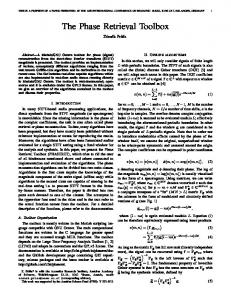
4.. Experiments and perform mance of the e parallel LS3 3U allgorithm The proposed G-LS3U G algorithm is parallelized ass described in Secc. 3, nd coded and com mpiled with Visua al C++ 2013 and CUDA 8.0. In ord der an to compare the accceleration perfo ormance, besidess the convention nal MA ATLAB impleme entation [19], a CPU multi-core implementation is alsso developed wiith the following g optimizations: (i) ( OpenMP [37] is ussed as the threadiing library to parrallelize the loop shown s in Fig. 2; (ii) ( LA APACK routine ?sysv ? optimized by b the Intel’s Maath Kernel Libraary (M MKL) [38] is used d to solve the line ear equation systtems in Eq. (6); (iiii) the good practicess proposed in [2 22] for implemeenting a multi-co ore W WFF algorithm arre also employe ed. All tests aree performed on n a wo orkstation equip pped with an Inte el® Xeon® E5-1 1650 CPU (6 cores, 3.2 20 GHz main fre equency) and 16 6.0 GB RAM. Bo oth a low-end GP PU (N NVIDIA GeForce GTX 680, 8 SMss with 1536 CUD DA cores and 2G GB RA AM) and a high-e end GPUs, (NVIDIA GeForce GTX 1080, 20 SMs wiith 25 560 CUDA cores and a 8GB RAM), are a used to verify y the computation nal peerformance of th he parallelization n. Two experimen nts are conducteed, co ompared, and exp plained below. 4.1 Dynamic fringge projection In the first exam mple, motion of a piece of A4 papeer is measured by ya dyynamic fringe prrojection profilom meter and recorrded with a vid deo caamera at the fram me rate of 30 fps. A sequence of 10 08 frames of frin nge paatterns is processsed, where the im mage size is 256×2 256 pixels [1]. Tw wo representative frin nge patterns of frrames 20 and 64 are shown in Figs. g extracted wrapp ped phase maps by 6aa and 6b, and their corresponding LSS3U are shown in Figs. 6c and 6d, 6 respectively. The T parameters of W WFF used are: σ x = σ y = 10 as recommended r [1 1]; accordingly, the t
due to the very small sspatial variation of the phase ch hange, and by consideering the energyy leakage [1], th he frequency baand is set as
ξl = −3ξi = −0.3 , ξh = 3ξi = 0.3 , ηl = −3ηi = −0.3 ,
and
η h = 3η i = 0.3 . The setting of these parameterss affects the computting speed. A threeshold thr is also o needed in WFF but its setting does noot affect the comp puting speed. Acccording to the disscussion in [1], thr = 5 iis used in this exa xample. Different implementationss of LS3U give the sam me extracted phasse.
Fig. 6. LS3U for fringee projection proffilometry: (a) an nd (b): fringe pattern ns at two represeentative frames; (c) and (d) the ccorresponding wrappeed phase maps exxtracted by LS3U.. The eexecution time co osts of the MATLA LAB sequential LSS3U, the multicore CP PU implementattion, and G-LS3U U are listed in Table 1. The MATLA AB implementatio on has the slowesst speed of 0.4 fp ps. (This speed is loweer than the previ vious test in [20]], which is reaso onable due to differen nt parameter settting.) The multii-core CPU impleementation is able too execute at 10 0.1 fps, which iss still slower th han the data acquisittion speed. On th he other hand, tthe low-end GTX X 680 and the high-en nd GTX 1080 GPU Us achieve 64.5 ffps and 131.8 fpss, respectively, which aare much higherr than the data aacquisition speed d. GTX 1080 is more th han 2 times fastter than GTX 680 0 because it con ntains a larger numberr of SMs such thaat more data can n be processed in n parallel. The computtational performaance of each step p in Algorithm 3 is provided in Table 2 for further exam mination. Stepss 0&6: The meemory transfer between CPU and GPU, as expecteed, only occupiess a very small p portion of the ovverall running time byy utilizing page-locked memory [26]; parallelized leasst-squares fittin ng algorithm Stepss 1-3: The p perform med on GTX 1080 0 only takes less tthan 1ms, which is very fast. In fact, as illustrated in Secction 3.2, this fasst speed mainly benefits from the prop posed parallel so olver used to solvee the linear equattion system in Eq. (7). Table 3 further ccompares the com mputation speed of the parallel solver w with the MATLA AB and CPU multti-core implemen ntations of the same allgorithm. Compaared with the CP PU multi-core implementation, the speeedup ratios of 13 35.42 and 367.57 7 are achieved byy the GTX 680 and GTX X 1080, respectivvely. Step 4: The WFF den noising process d dominates the ovverall running time of G-LS3U, and it iss more than an orrder of magnitud de longer than the sum m of the other step ps. The comparisson of the MATLA AB, CPU multicore, an nd GPU implemeentations of WFF F algorithm is givven in Table 3. Comparred with the CP PU multi-core implementation, the speedup ratios oof 4.77 and 11.23 3 are achieved byy the GTX 680 an nd GTX 1080, respecti tively. Step 5: The computattion of the phase change and the ccurrent phase also coosts a very sm mall portion off the overall rrunning time.
saampling intervalss are set as ξi = 1/ σ x = 0.1 and d ηi = 1 / σ y = 0.1 ; T Table 1. Comparrison of the averrage running tim me and frame rattes among the M MATLAB, the CP PU Multi-core, an nd the proposed d GPU-based im mplementations of LS3U of the fi first example. Speedup Ratio MATLAB CPU 6-coree GTX 680 0 080 GTX 10 GTX 68 80 vs. GTX 1 1080 vs. (s/fps) (s/fps) (s/fps)) (s/fp ps) CPU 6--core CPU 6-core 279.1/0.4 10.7/10.1 1.7/64.5 5 0.8/13 31.8 6.4 4 1 13.0
Table 2. Av verage running time t of each step p of G-LS3U on o one image fram me of the first exa ample. GTX 680 GTX 1080 Step (ms) (ms) 0 0.023 0.012 1 0.165 0.065 2 0.191 0.072 3 0.017 0.017 14.631 6.216 4 0.020 0.010 5 0.048 0.028 6 Ta able 3. Compariison of the avera age computation n time of solving g the linear systtems (Eq. (7)) an nd WFF among tthe MATLAB, th he CPU multicore, c and the pro oposed GPU-bassed implementaations on the firrst example. Speedup Ratio MATLAB CPU 6-Core GTX 680 GTX X 1080 GTX 6 680 vs. GTX 1080 vs. Operation n (ms) (ms) (ms) (m ms) CPU 6 6-Core CPU 6 6-Core Solving Eq. (7) ( 558.20 25.73 0.19 0 0.07 135 5.42 367 7.57 WFF 372.61 70.06 14.68 6 6.23 4.77 11 1.23 4.22 Dynamic speckle shearograph hic interferomettry In the second exxample, deformattion of a fully clam mped circular plaate is measured by a dynamic d speckle e shearographic interferometer i an nd recorded with a vid deo camera at the e frame rate of 30 0 fps. A sequencee of 11 17 frames of speckle patterns is processed, p wherre the image sizee is 36 66×371 pixels [1]]. Two representa ative speckle corrrelation patternss of fraames 40 and 10 04 which are obtained o by subttracting the inittial sp peckle pattern frrom them, are shown in Figs. 7a and 7b. Theeir co orresponding extrracted wrapped phase maps by LS3U L are shown in Figgs. 7c and 7d, respectively. Th he parameters of o WFF used arre: hich is larger due to the heavy noisse; accordingly, the t σ x = σ y = 20 wh saampling intervals are set as ξi = ηi = 0.05 , and thee frequency band d is seet as ξl = ηl = −0.15 , and ξ h = ηh = 0.15 . The threshold is set as thr = 10. The trend of the computational performance is similar to the firrst exxample. Howeverr, because (i) com mpared with thee first example, the t seecond example do oubles the pixel number, and (ii)) the WFF windo ow sizze is also double ed, the frame rattes achieved by GTX 680 and GT TX 10 080 are 31.8 fps and a 53.7 fps, which are slower thaan those in the firrst exxample. The MA ATLAB and the CPU multi-coree implementatio ons acchieve 0.2 fps and d 3.6 fps, respectiv vely.
5. Con nclusions A reaal-time GPU-baseed LS3U (G-LS3U U) algorithm is p proposed and implem mented for dynam mic phase retrieeval from fringee and speckle pattern ns. Real-time fram me rates of up tto 64.5 fps and 131.8 fps are achieveed in processing image frames ccontaining 256×2 256 pixels on NVIDIA A’s GTX 680 and d GTX 1080 GP PUs, respectivelyy. It is worth mention ning that, the pro oposed optimizaation of the wind dowed Fourier filteringg (WFF) algorith hm has also beeen tested on sim mulated fringe pattern ns with 1024×1 1024 pixels usin ng the same paarameters as ned in Section 4.1. An averagee computation sspeed of 75.8 mention ms/fram me has been acchieved on NVIIDA’s GTX 1080 0. Since WFF dominaates the overall ru unning time of G--LS3U, it can be eestimated that the prop posed method caan still run with a high framerate aaround 13 fps under ssuch a high ressolution. Even h higher frames rrates may be achieveed by adjusting the WFF param meters if prior k knowledge is known on the experimeent. Also, in pracctice, higher-end GPUs such as A’s GTX 1080 are preferred, not on nly for its greaterr computation NVIDIA efficienccy, but also for laarger graphical m memory capacity (8GB for GTX 1080), which is necesssary for holdingg and processingg larger-scale images.. Fundin ng Information. Singapore Acaademic Research h Fund Tier 1 (RG28//15).
Refereences 1. 2.
Figg. 7. LS3U for speckle shearog graphic profilom metry: (a) and (b b): sp peckle correlation n patterns at two o representative frames; f (c) and (d) ( the corresponding wrapped phase maps m extracted by b LS3U. As the WFF deno oising process do ominates the overrall running timee of G--LS3U, the settin ng of WFF param meters becomess important and is wo orth a discussion n. If we have no prior p knowledge on the experiment, the setting in the e second example, which is general g enough, is w know that the experiment only y has mild noise, the t recommended. If we seetting in the firstt example is suittable for higher acceleration. If we w haave even better knowledge k on the e experiment, furtther adjustment on the parameters can n be attempted
3.
4.
5.
6.
Q. Kemao, Winndowed Fringe Patttern Analysis (SPIE Press Bellingham, W Wash, USA, 2013). G. H. Kaufmann, aand D. Kerr, "Phasee-shifted J. M. Huntley, G dynamic speckkle pattern interferrometry at 1 kHz,"" Applied optics 38, 65566-6563 (1999). J. Millerd, N. B rock, J. Hayes, M. North-Morris, B. K Kimbrough, mask dynamic inteerferometers," and J. Wyant, ""Pixelated phase-m in Fringe 2005 (Springer, 2006), pp. 640-647. nkena, "Real-time displacement A. J. van Haast eren and H. J. Fran measurement using a multicameera phase-stepping speckle interferometerr," Applied optics 33, 4137-4142 (19994). C. Joenathan, B B. Franze, P. Haible, and H. Tiziani, ""Speckle interferometryy with temporal ph hase evaluation fo or measuring large-object deeformation," Applied optics 37, 26088-2614 (1998). C. Joenathan, B B. Franze, P. Haible, and H. Tiziani, ""Large in-plane displacement m measurement in d dual-beam specklee interferometryy using temporal p phase measurement," journal of modern optics 45, 1975-1984 (1998).
7.
8.
9.
10.
11.
12.
13.
14.
15.
16.
17.
18.
19.
20.
21.
22.
23.
24.
25.
G. H. Kaufmann and G. E. Galizzi, "Phase measurement in temporal speckle pattern interferometry: comparison between the phase-shifting and the Fourier transform methods," Applied optics 41, 7254-7263 (2002). V. Madjarova, H. Kadono, and S. Toyooka, "Dynamic electronic speckle pattern interferometry (DESPI) phase analyses with temporal Hilbert transform," Optics express 11, 617-623 (2003). F. A. M. Rodriguez, A. Federico, and G. H. Kaufmann, "Hilbert transform analysis of a time series of speckle interferograms with a temporal carrier," Applied optics 47, 1310-1316 (2008). X. C. de Lega, "PROCESSING OF NON-STATIONARY INTERFERENCE PATTERNS: ADAPTED PHASE-SHIFTING ALGORITHMS AND WAVELET ANALYSE. APPLICATION TO DYNAMIC DEFORMATION MEASUREMENTS BY HOLOGRAPHIC AND SPECKLE INTERFEROMETWY," (ÉCOLE POLYTECHNIQUE FÉDÉRALE DE LAUSANNE, 1997). A. Federico and G. H. Kaufmann, "Robust phase recovery in temporal speckle pattern interferometry using a 3D directional wavelet transform," Optics letters 34, 2336-2338 (2009). Y. Fu, R. M. Groves, G. Pedrini, and W. Osten, "Kinematic and deformation parameter measurement by spatiotemporal analysis of an interferogram sequence," Applied optics 46, 8645-8655 (2007). T. E. Carlsson and A. Wei, "Phase evaluation of speckle patterns during continuous deformation by use of phase-shifting speckle interferometry," Applied optics 39, 2628-2637 (2000). L. Bruno and A. Poggialini, "Phase shifting speckle interferometry for dynamic phenomena," Optics express 16, 4665-4670 (2008). W. An and T. E. Carlsson, "Speckle interferometry for measurement of continuous deformations," Optics and lasers in engineering 40, 529-541 (2003). Y. H. Huang, S. P. Ng, L. Liu, Y. S. Chen, and M. Y. Hung, "Shearographic phase retrieval using one single specklegram: a clustering approach," Optical Engineering 47, 054301-054301054305 (2008). Y. Huang, F. Janabi-Sharifi, Y. Liu, and Y. Hung, "Dynamic phase measurement in shearography by clustering method and Fourier filtering," Optics express 19, 606-615 (2011). Q. Kemao, "Two-dimensional windowed Fourier transform for fringe pattern analysis: principles, applications and implementations," Optics and Lasers in Engineering 45, 304-317 (2007). L. Kai and Q. Kemao, "Dynamic phase retrieval in temporal speckle pattern interferometry using least squares method and windowed Fourier filtering," Optics express 19, 18058-18066 (2011). L. Kai and Q. Kemao, "Dynyamic 3D profiling with fringe projection using least squares method and windowed Fourier filtering," Optics and Lasers in Engineering 51, 1-7 (2013). W. Gao, N. T. T. Huyen, H. S. Loi, and Q. Kemao, "Real-time 2D parallel windowed Fourier transform for fringe pattern analysis using Graphics Processing Unit," Optics express 17, 2314723152 (2009). M. Zhao and Q. Kemao, "Multicore implementation of the windowed Fourier transform algorithms for fringe pattern analysis," Applied Optics 54, 587-594 (2015). W. Gao, Q. Kemao, H. Wang, F. Lin, and H. S. Seah, "Parallel computing for fringe pattern processing: A multicore CPU approach in MATLAB® environment," Optics and Lasers in Engineering 47, 1286-1292 (2009). W. Gao, K. Qian, H. Wang, F. Lin, H. S. Seah, and L. S. Cheong, "General structure for real-time fringe pattern preprocessing and implementation of median filter and average filter on FPGA," in Ninth International Symposium on Laser Metrology, (International Society for Optics and Photonics, 2008), 71550Q71550Q-71558. W. Gao, "Real‐time pipelined heterogeneous system for windowed Fourier filtering and quality guided phase
26. 27. 28.
29. 30.
31. 32. 33.
34. 35. 36.
37.
38.
unwrapping algorithm using Graphic Processing Unit," in INTERNATIONAL CONFERENCE ON ADVANCED PHASE MEASUREMENT METHODS IN OPTICS AND IMAGING, (AIP Publishing, 2010), 129-134. C. Nvidia, "Nvidia cuda c programming guide" (2016), retrieved https://docs.nvidia.com/cuda/cuda-c-programming-guide/. Z. Malacara and M. Servin, Interferogram analysis for optical testing (CRC press, 2016), Vol. 84. Z. Wang and B. Han, "Advanced iterative algorithm for phase extraction of randomly phase-shifted interferograms," Optics letters 29, 1671-1673 (2004). Q. Kemao, "Windowed Fourier transform for fringe pattern analysis," Applied Optics 43, 2695-2702 (2004). W. Gao and Q. Kemao, "Parallel computing in experimental mechanics and optical measurement: a review," Optics and Lasers in Engineering 50, 608-617 (2012). D. B. Kirk and W. H. Wen-mei, Programming massively parallel processors: a hands-on approach (Newnes, 2012). S. Cook, CUDA programming: a developer's guide to parallel computing with GPUs (Newnes, 2012). T. Wang, Z. Jiang, Q. Kemao, F. Lin, and S. Soon, "GPU Accelerated Digital Volume Correlation," Experimental Mechanics 56, 297-309 (2016). B. N. Datta, Numerical linear algebra and applications (Siam, 2010). C. Nvidia, "CUFFT library user's guide" (2014), retrieved http://docs.nvidia.com/cuda/cufft/. M. Abdellah, "cufftShift: high performance CUDA-accelerated FFT-shift library," in Proceedings of the High Performance Computing Symposium, (Society for Computer Simulation International, 2014), 5. L. Dagum and R. Menon, "OpenMP: an industry standard API for shared-memory programming," Computational Science & Engineering, IEEE 5, 46-55 (1998). E. Wang, Q. Zhang, B. Shen, G. Zhang, X. Lu, Q. Wu, and Y. Wang, "Intel math kernel library," in High-Performance Computing on the Intel® Xeon Phi™ (Springer, 2014), pp. 167188.