Jun 2, 2003 - Rajeev Alur, Costas Courcoubetis, and David Dill. Model-checking for ... Alexandre David, Oliver Möller, and Wang Yi. Formal Verification of ...
Real-Time Statechart Semantics Holger Giese1 and Sven Burmester2 Software Engineering Group University of Paderborn Warburger Str. 100, D-33098 Paderborn Germany [hg,burmi]@uni-paderborn.de 2nd June 2003
Abstract Modelling complex dynamic real-time behavior is a crucial prerequisite when employing object-oriented modelling techniques successfully in the field of complex real-time systems. In this report we therefore review the state of the art of two related lines of research, namely extensions for expressiveness such as Statecharts as proposed in the field of software engineering to support the description of complex behavior and extensions to specify the explicit temporal behavior for state-based behavior such as Timed Automata. We review the Hierarchical Timed Automata model which provides already the most fundamental concepts for structure and time as well as a reasonable semantics for the domain of temporal behavior. To enable the modeling of complex control behavior which incorporates most of the fundamental extensions for expressiveness and time in a manner appropriate for real-time systems, we then propose an extension in form of Extended Hierarchical Timed Automata and Real-Time Statecharts. Different restricted forms reflecting the different requirements of system elements such as physical entities, communication channel abstractions and controllers running on particular platforms are further identified.
Keywords: Real-Time Statecharts, Hierarchical Timed Automata, Timed Automata, real-time systems, distributed systems, behavior specification.
1 supported by the german research council (DFG) within the collaborative SFB 614 named ”Self-optimizing Concepts and Structures in mechanical Engineering” 2 supported by the International Graduate School of Dynamic Intelligent Systems.
Contents 1 Introduction
3
2 Requirements 2.1 Real-Time Systems . . . . 2.2 Expressiveness . . . . . . 2.3 Temporal Behavior . . . . 2.4 Predictability . . . . . . . 2.4.1 Feasibility Analysis 2.4.2 Formal Verification 2.5 Realizability . . . . . . . .
. . . . . . .
. . . . . . .
. . . . . . .
. . . . . . .
. . . . . . .
. . . . . . .
. . . . . . .
. . . . . . .
. . . . . . .
. . . . . . .
. . . . . . .
. . . . . . .
. . . . . . .
. . . . . . .
. . . . . . .
. . . . . . .
. . . . . . .
. . . . . . .
. . . . . . .
. . . . . . .
. . . . . . .
. . . . . . .
. . . . . . .
. . . . . . .
. . . . . . .
. . . . . . .
. . . . . . .
. . . . . . .
. . . . . . .
. . . . . . .
. . . . . . .
. . . . . . .
3 3 4 5 6 6 6 7
3 Timed Automata 3.1 Timed Automata 3.2 Consistency . . . 3.3 Extensions . . . . 3.4 Summary . . . .
. . . .
. . . .
. . . .
. . . .
. . . .
. . . .
. . . .
. . . .
. . . .
. . . .
. . . .
. . . .
. . . .
. . . .
. . . .
. . . .
. . . .
. . . .
. . . .
. . . .
. . . .
. . . .
. . . .
. . . .
. . . .
. . . .
. . . .
. . . .
. . . .
. . . .
. . . .
. . . .
8 9 10 11 12
4 Hierarchical Timed Automata 4.1 Syntax . . . . . . . . . . . . . . . . . . . . . . . . . . . . . . . . . . . . . . . . . . . 4.2 Semantics . . . . . . . . . . . . . . . . . . . . . . . . . . . . . . . . . . . . . . . . . 4.3 Summary . . . . . . . . . . . . . . . . . . . . . . . . . . . . . . . . . . . . . . . . .
12 12 14 17
5 Extended Hierarchical Timed Automata 5.1 Extensions . . . . . . . . . . . . . . . . . . 5.2 Syntax . . . . . . . . . . . . . . . . . . . . 5.3 Semantics . . . . . . . . . . . . . . . . . . 5.4 Summary . . . . . . . . . . . . . . . . . .
. . . .
. . . .
. . . .
. . . .
. . . .
. . . .
. . . .
. . . .
. . . .
. . . .
. . . .
. . . .
. . . .
. . . .
. . . .
. . . .
. . . .
. . . .
. . . .
. . . .
. . . .
. . . .
. . . .
17 17 18 20 24
6 Real-Time Statecharts 6.1 Extension . . . . . . 6.2 Semantics . . . . . . 6.3 Realizability . . . . . 6.4 Summary . . . . . .
. . . .
. . . .
. . . .
. . . .
. . . .
. . . .
. . . .
. . . .
. . . .
. . . .
. . . .
. . . .
. . . .
. . . .
. . . .
. . . .
. . . .
. . . .
. . . .
. . . .
. . . .
. . . .
. . . .
24 24 25 27 27
. . . .
. . . .
. . . .
. . . .
. . . .
. . . .
. . . .
. . . .
. . . .
. . . .
. . . .
. . . .
. . . .
. . . .
. . . .
. . . .
. . . .
7 Related Work
28
8 Conclusion
29
3
1
Introduction
To model complex reactive real-time systems, state machine specification techniques are one successful approach. However, they have to face a number of problems. On the one hand, a number of extensions for the expressiveness of state machines such as Statecharts [Har87] have been proposed in the field of software engineering to support the description of complex behavior. On the other hand, to specify the required temporal behavior for state-based behavior well-founded formal concepts such as Timed Automata have to be employed. While both research directions have their own merits, a combination of both worlds has to face serious problems. The Statechart extensions for structure and micro- and macro-steps which achieve the required degree of expressiveness assume an infinite fast machine and therefore assumes that the environment will not interfere with its execution. In contrast to this approach assumes the Timed Automata models and related research that temporal properties of the automaton are explicitly modeled to study whether the temporal behavior is appropriate. To obtain an applicable solution for developing real-time control software, it is further required that the specification formalism can be analyzed to proof the required properties (predictability) and used to derive a correct operating software (realizability). We will show that current proposals are not able to cover all four requirements and therefore present a solution that takes expressiveness, temporal behavior, realizability and predictability into account. First, the basic characteristics of real-time systems and the resulting main requirements for an applicable description technique are identified in Section 2. Then, we review the underlying notion of Timed Automata and its foundations in Section 3. This includes the basic principles of state machines and its extension to the notion of Timed Automata. Extensions with the concepts of Statecharts for expressiveness as proposed with the notion of Hierarchical Timed Automata are then reviewed and defined in Section 4. In Section 5 (ExHTA) the syntax and semantics for the proposed extension in form of the extended hierarchical timed automata model which takes into account all four aspects and addresses the most of the crucial issues identified in Section 2 is described. The report closes with some final conclusion in Section 8.
2
Requirements
To identify the relevant requirements for a temporal state-based formalism that serves expressiveness as well as temporal aspects, we start with reviewing what are the main characteristics and obstacles to modelling of real-time systems in Section 2.1. In Section 2.2 we further review which main structural modelling extensions proposed in the software engineering context are appropriate in the specific domain of real-time systems. Besides reactive behavior and complex state spaces of course the temporal behavior is another prerequisite discussed in Section 2.3. Then the specific question of predictability is addressed in Section 2.4 looking on the analysis opportunities for different timed models. Efforts for the higher-level specification of a system are only reasonable, when the realizability of the concepts as reflected in Section 2.5 is also taken into account.
2.1
Real-Time Systems
Activities within a real-time system are described by a number of independently running tasks that interact with the environment. Tasks can be classified as hard real-time, soft real-time or non real-time constrained relating to a so called utility function. For a hard real-time task the value (utility) of a required result or effect will be zero after its deadline has been passed. For a soft real-time task the value decreases after passing the deadline and for non real-time tasks no deadline effecting the value of the task is given at all.
4
2
REQUIREMENTS
In general, a real-time system is composed of 3 layers: The hardware, the real-time operating system (RTOS) and the software. The hardware consists of one or multiple controllers and optional resources like memory, sensors or actuators. The RTOS is the interface between hardware and software and provides operations for accessing the resources. In every operating system, all concurrently running tasks try to access the controllers and the resources simultaneously. As every controller can handle only one task, the operating system provides a taskmanager to regulate this access. RTOS provide a so called scheduler as taskmanager, trying to meet the deadlines of the regulated tasks. When accessing shared resources, concurrent access has to be controlled, e.g. in order not to read from and write to a shared resource at the same time. Therefore, for modelling hard real-time systems it is crucial to have appropriate means to express temporal constraints. While this can be done rather straight forward at the theoretical levels each concrete device can only execute with limited speed and therefore besides specifying what time properties are expected we still have to ensure that the resulting tasks do also meet their deadlines. For hard real-time systems therefore predictability is required. Usually this in only possible when for alternatives simply the worst-case is considered. E.g., usually all tasks are viewed on only by taking their worst-case execution time (WCET) into account. The reactive nature of most hard real-time systems further make periodic operating tasks the underlying paradigm for real-time systems. Therefore, often multiple independent tasks scheduled either by a real-time operating system (RTOS) or run-time system are employed. The scheduling can be realized using pre-computed static schedules, e.g. controlled by a priority scheduler. Using this scheduler, a priority is assigned to every task determining the order of execution. Note, that even for a single threaded system with explicit ordering of tasks, the resulting worst- and bestcase execution give lower or upper bounds on their periodic occurrence which permits to estimate whether the required deadlines will be met. As outlined above, controllers have to cope with the described restrictions, while real world physical entities may behave arbitrary fast. Therefore, a notion for temporal state-based behavior should permit to distinguish both kinds of models and detect whether a model can be executed on a limited device or is a physical abstraction that cannot be realized by a controller. We further name these two different kinds of models • limited , if they can be realized on a man made digital controller or • unlimited , if they describe the behavior of a physical device that cannot be realized on a man made digital controller. It is to be noted, that certain abstractions might result in a mix of both models. A communication subsystem, for example, consists besides the technical components and software of a transmission media or channel which may result in possible failures or delays that result in an unlimited behavior. For a given hardware, a limited model might still be realizable or not depending on its resource requirements.
2.2
Expressiveness
To support the design of complex reactive behavior statecharts [Har87] extended the flat unstructured control state space of traditional finite state machines by supporting specific concepts such as hierarchy, parallel AND-states and deep and shallow history states. Therefore, rather complex state-based behavior can often be described in a compact form. Note that besides modelling comfort also the expressiveness of automata models with or without concepts like AND states vary. Therefore the number of required states to model a specific complex behavior depends on the availability of these higher-level description concepts (cf. [DH94]).
2.3 Temporal Behavior
5
For Statecharts the temporal behavior can be specified by the after and when constructs. A transition labeled with after(x) fires x time units after entering the source state, when(x) fires at point x in time. So after is used for the declaration of a relative date, when for an absolute. In this form, support of an unlimited device is needed to identify the point of times without delay. Besides these explicit constructs which permit to describe timeout behavior as required for the real-time domain, the temporal behavior of Statecharts is usually not specified. Thus for all side-effects and required computations no timing information is present. Statecharts abstract from concrete timing information and assume an infinite fast device. As outlined in the preceding part about real-time systems, for a controller such an assumption is not realistic. In practice the assumption can be reduced by simply stating that the Statechart is executed fast enough to react on all relevant environment changes. Fast enough is difficult to determine and a model is required that somehow also represents this information. Therefore, an extension with explicit timing information is required. In the case of the UML state machine [Obj01] the related micro- and macro-step execution order has been adjusted to ensure that the machine does first compute all internal effects of a received event (run-to-completion) before new external events are considered. While this simplifies the implementation of UML state machines on the other hand the delay in reaction to external events can be rather prohibitive for a real-time system. Therefore, when looking for an appropriate realtime modelling notation we have to keep in mind that reasonable worst-case reaction time may be in conflict with some features of the macro- and micro-step semantics and run-to-completion semantics.
2.3
Temporal Behavior
In real world physical entities operations are time-consuming. When they are executed on a limited device, their maximum duration is denoted by the worst case execution time (WCET). Deadlines are used to specify that an action has to finish its execution in the given time bound. Typically automata are implemented by a control task, that checks periodically the activation of transitions. So an activated transition is not fired at the point of activation, but rather during the following period of the control task. This results in a delay, caused by the limitation of the device. Specification of the deadline gives – w.r.t. the WCET – an upper bound for the acceptable delay. When deadlines and WCETs are specified, well-known methods and algorithms can be used to determine if a schedule exists, affecting that all deadlines are met, and to determine this schedule; e.g. using a priority scheduler and assigning the priorities according to the Deadline Monotonic Priority Assignment. The employed notion of time in a real-time system is usually limited by the maximal clock resolution of the underlying RTOS or hardware. Therefore, the clock values we can compare in a program can always be encoded by a countable set of time points. When instead of absolute clock values only relative time differences are used, a straight forward extension of an automata models towards discrete time exists where different clock values are used to determine time-dependent behavior. However, when using such clock values this usually does not include the assumption that time elapses only in discrete steps. Instead a clock value n is assumed to represent the interval [n, n + 1) rather than a discrete point in time. Therefore, the read clock values and clock value comparisons check whether upper or lower bounds actually hold for a clock value and the underlying interpretation is that the clock therefore is in the time interval determined by the corresponding interval.
6
2.4
2
REQUIREMENTS
Predictability
The required support for predictability can vary to a great extent. Traditionally, the periodic nature of all real-time tasks is exploited to predict whether all deadlines will be met (feasibility analysis). If more specific system properties should be predicted or the assumption of independent periodic tasks is not valid, however, other techniques for automatic formal verification such as model checking may be employed.
2.4.1
Feasibility Analysis
Most approaches to real-time system design support a feasibility analysis to check whether a given set of periodic tasks can be served in a manner that all deadlines are met. As there are many different kinds of schedulers, for every approach exist different algorithms, for checking the feasibility. Scheduling can be preemptive or non-preemptive, static or dynamic. One widespread manner is the static, preemptive priority scheduling. Using this scheduler, a priority is assigned to every task. Whenever the scheduler is assigning tasks to processors and has to distinguish between multiple tasks, it chooses the one with the highest priority. If the processor is busy with a low priority task and a high priority task arrives, then the active task is preempted and the processor is assigned to the task with the higher priority. When it is possible to change the priorities during runtime, the scheduling is called dynamic, otherwise static. Thus, the feasibility of a set of tasks strongly depends on the manner of priority assignment. The Rate Monotonic Approach (RMA) [BR99], that assigns higher priorities to tasks with shorter periods, results in an optimal scheduling. That means, that the set of tasks, having rate monotonic priorities, is schedulable, if any priority assignment exists, that makes the set schedulable. RMA is limited to periodic tasks. A set of tasks, containing aperiodic tasks, the Deadline Monotonic Priority Assignment [BW01] (a task with a short deadline achieves a high priority), is optimal. Both approaches are static, as the priorities are computed in advance of starting the tasks and are not changed during runtime. As these approaches are widespread, there exist a couple of algorithms for accomplishing a feasibility analysis. The theorems from Liu and Layland resp. Lehocky, Sha and Ding [BR99] confirm the feasibility of a set of tasks scheduled by RMA. In [Jos96] an algorithm is presented, accomplishing an analysis for priority scheduling independent of the manner of priority assignment. In general, different tasks may access the same resources (like memory). Obviously, the access to these shared resources, has to be controlled as there will be problems, when a task, writing to a memory address, is interrupted by an higher prioritized thread, which writes to the same address. To avoid this problem a task, accessing a shared resource, blocks all (higher prioritized) tasks, that try to access this resource. Unfortunately, this solution results in an effect called Priority Inversion. This occurs when due to blocking the highest prioritized task finishes its execution at last (see [Jos96, BR99] for a complete example). Because of this effect, protocols have been investigated to minimize the blocking times. Widespread protocols are the Priority Inheritance Protocol and the Priority Ceiling Emulation [BR99].
2.4.2
Formal Verification
A behavioral modelling technique with well defined semantics permits to analyze the required temporal model properties using, e.g., temporal logic [Pnu77]. Given a specification in a temporal logic φ and a model M there exist a number of techniques to prove that the model fulfils the
2.5 Realizability
7
specification (M |= φ). Following [Lam77] such specifications can be further separated into safety and liveness conditions. While safety conditions ensure that something bad never happens, do liveness conditions ensure that something good will happen. Note, that thus liveness includes progress (something will happen). The basic notion of temporal logic does only cover causal ordering, but does not permit to express properties with explicit real-time constraints. Therefore, a number of extensions with different time models have been proposed. A first natural approach is to employ and extend available techniques for un-timed systems such as model checking. If a countable set of time points are sufficient a discrete notion of time can be used where, for example, the natural numbers denote all possible time points. When instead of absolute values only relative time differences are used, a straight forward extension of an automata model towards discrete time exists and available techniques for its analysis can be employed (cf. [EMSS90]). A Tool for such a discrete timed model is, for example the model checker RAVEN [RK99, RK00] which employs clocked computation tree logic (CCTL) as specification language. For a timed step with a delay of more than one minimal time unit in such a discrete interpretation of time the question arises what is the correct interpretation of the intermediate states. Do these intermediate states correspond to ”copies” of the source state , ”copies” of the target state, or is in fact nothing known about these intermediate states. Therefore, in [LS01] a temporal logic and related model checking techniques are proposed that assume the latter while in RAVEN the first case is assumed. However, the assumption that time elapses only in discrete steps is rather strong. A more serious problem in practice is to chose a sufficient small minimal discrete time value. On the one hand the choice has to ensure that the above assumption of a correct time abstraction holds. On the other hand the applicability of analysis techniques crucially depends on a chosen minimal discrete time value large enough. Therefore a systematic way to determine such a minimal discrete time value is required, before these approaches can be safely employed to automatically predict and analyze the required system properties. As outlined in [HNSY92], when a digital clock value n is assumed to represent the interval [n, n+1) rather than a discrete point in time, for restricted cases of models or temporal logic formulas results proven for the digitalization will also hold for the more realistic continuous time model. When also stronger specifications in the digital model are used and the digitization granularity is refined we can further approximate step-wise the required continuous time property. To further automate this task, an approach that automatically determines a finite abstraction of a given real-time system is more appropriate than a manual approximation. For a continuous model of time, timed automata [AD90] as automata theoretic approach provides such a solution. It supports continuous clocks and employs the property that the clocks are only tested for a finite number of rational constants for only rational constants to construct of a finite abstraction in form of a region-graph (cf. [AD90]). With COSPAN [AK96], HyTECH [HHWT95a], KRONOS [DOTY96], and UPPAAL [LPY97, PL00] a number of tools for model checking Timed Automata exist. Some of them further support hybrid and parameterized verification.
2.5
Realizability
A real-time system consists of hardware (controller, resources, actuators, sensors etc.) and its software. Concerning the integration between software and hardware there are 2 common platforms: (1) a real-time operating system (RTOS) is used to decouple the real-time application from the hardware and (2) the special I/O architecture of a micro-controller is directly employed to connect
8
3
TIMED AUTOMATA
the real-time application with its environment. The advantages of the RTOS approach are that it provides operations with uniform access to the underlying hardware and can control the scheduling of multiple tasks which includes their access to the (shared) resources. Alternatively, when a micro-controller is employed, the whole logic of the application has to be covered by a single task. In this case the scheduler, respectively the RTOS, is not needed. One of the advantages of the multi-task architecture is, that the tasks can control each other and handle errors. In a single thread application, this is not possible. Real-time systems are often also embedded systems and thus besides the described heterogeneity w.r.t. scheduling also the available resources and execution restrictions can vary. When modelling a controller device these different forms (programmable logic controller (PLC), micro-controller (MC), and computer) restrict the delay and procedure the software can observe and control its environment. E.g., for PLC we usually have a bounded cycle time, while computer equipped with a RTOS permit a great variety of task periods which are served by the scheduler. For the considered case of high-level behavior models, a suitable mapping to an implementation is required. Whether a mapping is possible or not has thus to be detected also at the highlevel model. Otherwise, a delayed detection can result in rather wasted design efforts. Therefore, feasibility analysis at the level of the high-level behavior model is required.
3
Timed Automata
To discuss the foundations for extended state machine models for modelling temporal behavior, we introduce the required terminology and formal treatment by first reviewing the basic definition and terms for a finite automaton. The finite automaton is the most fundamental concept for state-based behavior. Their main elements are a finite set of control states (locations) denoted by S, a contained set of start locations S0 ⊆ S and a set of transitions T , where each t ∈ T further describes which changes between the locations are permitted depending either on internal choice or the environment. In a hardware oriented view the environment is modelled by input i ∈ I and output o ∈ O signals. The resulting output o can be further described either as function of S (Moore automata) or S and I (Mealy automata). In the considered software context instead a Mealy automata sending and receiving possible events a ∈ A rather than permanently provided input and output signals is usually employed. Definition 1 A finite automaton M is a 4-tuple (S, S0 , A, T ) with • S a finite non empty set of locations, • S0 ⊆ S the subset of start locations, • A a finite set of events including the internal event τ ∈ A. • T ⊆ S × A × S a finite set of transitions t = (s, a, s� ) ∈ T with – s ∈ S the source location, – a ∈ A the related action, and – s� ∈ S target location. a By convention for a transition t = (s, a, s� ) ∈ T we also write s → s� . Using S as the set of possible configurations the resulting transition system is as follows.
Definition 2 For a finite automaton M = (S, S0 , A, T ) the set of all possible configurations is simply S. The initial possible configurations are the elements of S0 . For a finite automate with
3.1 Timed Automata
9
current configuration l0 we further have the enabling condition Enabled(l0 , (l, a, l� )) ⇐⇒ (l0 = l) and related configuration transition function Γ(l,a,l� ) (l) := l� resulting in the following action rule: Enabled(l, t) action t l→ Γt (l) In the simply case of a finite automaton the distinction between the syntactical notion of the location set and the possible configurations is rather superficial. However, in the following we will study extended concepts for automata where both notions are not synonymous any more. As long as finite behavior is considered additionally often a set of accepting locations Sf ⊆ S is defined. The valid finite traces s0 a0→ s1 · · · sn with s0 , s1 , . . . , sn ∈ S ∗ are given by all finite sequence of transitions starting with any start location s0 ∈ S0 which end at an accepting location sn ∈ Sf (acceptance condition). For infinite traces s0 a0→ s1 · · · with s0 , s1 , . . . ∈ S ω , however, B¨ uchi automata [B¨ uc62] have to be used where instead for any possible infinite trace all states sa of the accepting location set Sa have to be visited infinite often (|{i|si = sa }| = ∞) to fulfill the acceptance condition. This way to describe acceptance of infinite behavior is rather elegant, however, not really intuitive when modelling a system. This mismatch is related to the following underlying fact: For the acceptance of finite or non finite regular languages in form of an automata angelic non-determinism [HU79] is employed, which essentially assumes that choices are always made with global knowledge. When modelling system behavior in a constructive fashion by composing multiple independently operating subsystems, however, erratic non-determinism [Bro86] is natural, where each subsystem is assumed to behave arbitrary.3 Therefore, a different technique to model the liveness and progress properties of the system is required when modelling systems rather than characterizing the acceptance of a language.
3.1
Timed Automata
Automata can be extended to also describe the temporal behavior using a continuous notion of time. The term timed automata also includes a number of automata theoretic approaches with real-value clocks. The main characteristic is that for the models often a finite abstraction can be constructed, which results in a number of related model checking approaches. One basic notion of Timed Automata also named timed graphs [ACD90] uses real-value clocks to further restrict the occurrence of transitions. This notion, however, does not exclude that the automata may idle forever in any reached configuration. The original proposal [AD90] avoids this problem extending the concepts of B¨ uchi automata [B¨ uc62] and thus accepts only such infinite runs which also infinitely often visits states marked as accepting. While this notion can be used to specify progress conditions in [HNSY92] a notion for Timed Automata also named timed safety automata is proposed that avoids to require accepting states and instead introduces clock constraints for control states to model progress guarantees explicitly. We will further use this last notion as basic notion of timed automata and refer to [AD94, Pet99] for more detailed overviews. The basic extension w.r.t. finite automata is that besides the control locations S a set of realvalue clocks C is also part of the transition system configuration in form of a clock binding ν ∈ Cν = [C → IR + ]. ν 0 is the special binding which assigns to each clock variable 0. To control the temporal behavior clock constrains Cc = [[C → IR+ ] → {true, false}] in form of time guards for transitions and time invariants for locations are employed. To reset the clock values as required specific clock updates Cu = [Cν → Cν ] are used. 3 For
a more detailed discussion on the different forms of non-determinism see [WM97].
10
3
TIMED AUTOMATA
Definition 3 A Timed Automaton M is a tuple (S, S0 , T, Inv, A, C) where • S a finite non empty set of locations, • S0 ⊆ L the subset of start locations, • Inv : S → Cc assigns each state a clock constraint, • A a finite set of events including the internal event τ ∈ A, • C a finite set of clocks and, • T ⊆ S × A × Cc × Cu × S a finite set of transitions t = (l, a, g, r, l� ) ∈ T with – l ∈ S the source location, – a ∈ A the related action, – g ∈ Cc a clock constraint named time guard, – r ∈ Cu a clock update, and – l� ∈ S target location. In the resulting transition system two forms of transitions are present. The transitions associated with each transition of T occur in a timeless step. Additionally, so called time steps which remain within the same control state (location) are possible where any arbitrary time delta d elapses. Definition 4 For a Timed Automaton M = (S, S0 , T, A, C) the state space is build by all pairs (l, ν) ∈ S × Cν . The initial possible states are all such pairs (l, ν 0 ) with l ∈ S0 . For a Timed Automaton in configuration (l, ν) we further define enabling by Enabled((l�� , ν), (l, a, g, r, l� )) ⇐⇒ l�� = l∧g(ν)∧Inv(l� )(r(ν)) and the resulting configuration transition Γ(l,a,g,r,l� ) (l, r(ν)) := (l� , r(ν)). Thus, for a transition t ∈ T the following action rule results: Enabled((l, ν), t) action. t (l, ν) → Γt (l, ν) Time can further elapse in so called delay steps and for the corresponding update function Γd ((l, ν)) := (l, ν + d), where ν + d stands for the current clock assignment plus the delay for all the clocks, we have Inv(l)(ν + d) delay. d (l, ν) → Γd (l, ν) Typically the updates and constraints for the continuous clock variables are further syntactically restricted to ensure that a finite abstraction [AD90] exists. For the transition updates Cu hold that clocks are usually only reset to 0 or integer numbers. For the time constraints in form of time invariants for locations and time guards for transitions usually the expressions are limited for x, y, clocks and constants n to the conjunctive combination of the form x✷n or x − y✷n with ✷ ∈ {}. For this restricted notion of time constraints the reachability problem for Timed Automata is decidable when the coefficients (n) in the guards are rational numbers [AD90]. The reachability problem becomes as soon undecidable as the coefficients are chosen, for example, from the set √ {1, 2} [Pur99]. When additive clock constraints are used, already for no more than 4 clocks the emptiness problem is in general undecidable [BD00].
3.2
Consistency
The described Timed Automata model can further result in subtle semantic problems. For example, for the employed notion of a Timed Automaton a configuration without any further possible timeless step named deadlock may be reached.
3.3 Extensions
11
Definition 5 A configuration (l, ν) is a deadlock iff ∀t ∈ T hold ¬Enabled((l, ν), t). A configuration without further external visible timeless steps still describes a reasonable behavior. If, however, the related time invariant of the control state (location) expires and further time elapses an inconsistent temporal behavior has been specified. Definition 6 A configuration (l, ν) is a time stopping deadlock iff it is a deadlock and for any d > 0 hold Inv(l)(ν + d) = false. Another problem of the presented approach to model continuous time behavior is caused by the employed interleaving of time steps and discrete action steps. While for arbitrary delta d and 0 0 1 d� time steps still describe a reasonable behavior, a sequence (l0 , ν0 ) d→ (l1 , ν1 ) t→ (l2 , ν2 ) d→ t1 (l3 , ν3 ) → (l4 , ν4 ) . . . with alternating time and action step is� not reasonable when infinitely many discrete action steps occur in a finite amount of time (∃d = ∞ i=1 di ). 0 1 2 Definition 7 An infinite sequence of configurations and steps (l0 , ν0 ) x→ (l1 , ν1 ) x→ (l2 , ν2 ) x→ x3 (l3 , ν3 ) → (l4 , ν4 ) . . . with xi ∈ (T ∪ IR + ) is considered to be zeno iff the�number |{i|xi ∈ T }| is infinite while for the elapsed time a finite upper bound d exists such that xi ∈IR + di ≤ d.
The problem of zeno behavior will usually only occur for unlimited systems, because there exists a lower bound tl for all the times required to execute a transition in a specific situation. Therefore, as long as besides the zeno behavior a reasonable non-zeno behavior exists it is usually assumed to simply exclude the traces with zeno behavior. When, however, unlimited systems and their physics is considered, the result of an infinite but convergent chain of transitions and time steps may indeed determine the correct behavior of the system.
3.3
Extensions
Besides this basic notion of Timed Automata several extensions have been proposed to simplify the specification of temporal behavior. For a configuration (l, ν) any enabled transition t may occur or not as long as the time invariant of the current location is valid. The only case when some transition will be executed definitely is when the invariant does not permit any further delay. Therefore, the concept of urgent transitions [HHWT95b, DY95, BLL+ 95] has been proposed where time can only elapse when no urgent transition is enabled. Formally for Tu ⊆ T the subset of all urgent transitions which are often further restricted to have empty guards (g = true) we can define whether an urgent transition is enabled UrgentEnabled((l, ν)) := ∃t ∈ Tu Enabled((l, ν), t) and simply adjust the delay rule accordingly. Inv(l)(ν + d) ∧ ¬UrgentEnabled((l, ν)) delay d (l, ν) → (l, ν + d) To simplify the modelling of complex state spaces besides explicit control states also integer variables [LPY97] have been invented. The resulting reachable system configurations simply have to include a binding for the variables, too. Note, that in the presented basic notion of Timed Automata the labels a ∈ A do not effect the execution of a transition. For a system of multiple parallel executed Timed Automata synchronous
12
4
HIERARCHICAL TIMED AUTOMATA
communication using channels in a Calculus of Communicating Systems (CCS) [Mil89] style has been proposed in [LPY97]. This permits to coordinate two parallel Timed Automata in a single atomic step. Two transitions with compatible channel events e! and e? are combined into a single transition of the combined system. Another way to let multiple parallel operating Timed Automata interact are shared variables [LPY97]. In contrast to the synchronous communication do shared variables facilitate an asynchronous exchange of information between parallel Timed Automata.
3.4
Summary
A system of Timed Automata with synchronous communication and shared variables provides already the required fundamental concepts to describe the complex real-time behavior of large systems consisting of a number of components. For reasonable small systems of Timed Automata model checking techniques further provide the required analysis and help to predict whether required properties hold. Therefore, the requirements temporal behavior and predictability are covered. However, the presented basic formalisms are still limited with respect to expressiveness and realizability. In the next section we therefore consider an approach that further extend the only flat structures supported by Timed Automata towards complex state spaces as supported by Statecharts.
4
Hierarchical Timed Automata
As identified in Section 2.2 the fundamental extensions to cope with complex behavior are hierarchy, parallelism and history as provided by statecharts [Har87] and its UML derivation UML state machines [Obj01]. The notion of a Hierarchical Timed Automata model [DMY02] provides the most fundamental structural concepts as well as a reasonable continuous time semantics. This notion supports model checking by a mapping to plain Timed Automata as employed in the UPPAAL tool [LPY95]. As part of the AIT-WOODDES research project a corresponding UML state machine profile is further planed. In the following we define Hierarchical Timed Automata as introduced in [DMY02] and summarize their exact limitations w.r.t. the in Section 2 identified requirements.
4.1
Syntax
Definition 8 A Hierarchical Timed Automaton is a tuple �S, S0 , δ, σ, V, C, Inv, Ch, T � where • S is a finite set of locations. root ∈ S is the root. • S0 ∈ S is a set of initial locations. • δ : S → 2S is a function, mapping a location l to all possible substates of l and generating a tree structure with root as the root. Applying δ on sets, delivers the intuitively expected results. • σ : S → {AN D, XOR, BASIC, EN T RY, EXIT, HIST ORY } associates a type to every location • V, C, Ch are sets of variables, clocks, and channels and are used for the specification of Guard, Reset, Sync, and Invariant as described in the following.
4.1 Syntax
13
• Inv : S → Invariant assigns an invariant to every location. • T ⊆ S × (Guard × Sync × Reset × {true, false}) × S is the set of transitions. A transition is composed of a source (l) and a target location (l� ), a guard g, an assignment r (including clock resets), and an urgency flag u. The notation l s,g,r,u→ l� is used for a transition t = (l, s, g, r, u, l�). We omit s, g, r, u when they are necessarily absent (or false, in the case of u). Guards, synchronizations, resets, and assignments use Guard, Reset and Sync, as described in the following: • V is the finite set of integer variables. V (l) ⊆ V is the set of integer variables local to a superstate l. • Let C be the finite set of clock variables. C(l) ⊆ C contains the clocks local to a superstate l. If l is a history state, C(l) contains only clocks, that are declared as forgetful. The other clocks of l (local clocks) belong to C(root). • Let Ch be the finite set of synchronization channels. Ch(l) ⊆ Ch contains the channels that are local to a superstate l, i.e., it is not possible to synchronize along a channel c ∈ Ch(l) between one transition inside l and one outside l. • Ch leads to the finite set of channel synchronizations( Sync). It holds: c ∈ Ch ⇒ c?, c! ∈ Sync. If s ∈ Sync, then s denotes the corresponding complementary(e.g. c! = c? and c? = c!). • Data constraints are boolean expressions of the form A✷A with A is an arithmetic combination of elements from V and ✷ ∈ {, =, ≤, ≥}. Clock constraints are boolean expressions of the form x✷n or x − y✷n, with x, y ∈ C, n ∈ N and ✷ ∈ {, =, ≤, ≥}. A clock constraint is called downward closed, if ✷ ∈ { p2 .
5.2
Syntax
These extensions result in the following definition for an Extended Hierarchical Timed Automata. Definition 10 The syntax of an Extended Hierarchical Timed Automaton is defined by a tuple �S, S0 , δ, σ, D, V, C, Inv, Ch, T � where • S is a finite set of locations. root ∈ S is the root. • S0 ∈ S is a set of initial locations. • δ : S → 2S . δ maps l to all possible substates of l. δ is required to give rise to a tree structure with root root. We readily extend δ to operate on sets of locations in the obvious way. • σ : S → {AN D, XOR, BASIC, EN T RY, EXIT, HIST ORY } is a type function on locations. • D, V, C, Ch are a data model, sets of variables, clocks, and channels. They give rise to Guard, Reset, Sync, and Invariant as defined in the following. • Inv : S → Invariant maps every location l to an invariant. • T ⊆ S × (Guard × Sync × Reset × IN ) × S is the set of transitions. A transition connects two locations l and l� , has a guard g, a synchronization s, an assignment r (including clock resets), and an priority p. We use the notation l g,s,r,p→ l� for this and omit g, s, r, p when they are necessarily absent (or 0, in the case of p). The data components in guards, synchronizations, resets, and assignment expressions are defined: • D is a possibly infinite data model. A set of possible queries [D → {true, false}] and transformations [D → D] are assumed. To further take into account that data model updates or queries cannot be considered to be timeless and atomic their interference has to be controlled in an appropriate manner. Therefore, we assume a symmetric function conflict that for an update up and an update or query up� determines whether their concurrent execution can result in such interference (conflict(up, up� ) = true). A conflict can be excluded between a guard and an update only, when the update cannot effect the outcome of evaluating the guard. For two updates in contrast, basic concurrency techniques such as monitors or semaphores may be employed to ensure interference free execution which is modelled by different forms of interleaving.
5.2 Syntax
19
• V is the finite set of integer variables. V (l) ⊆ V is the set of integer variables local to a superstate l. • Let C be a finite set of clock variables. The set C(l) ⊆ C denotes the clocks local to a superstate l. If l has a history entry, C(l) contains only clocks, that are explicitly declared as forgetful. Other locally declared clocks of l belong to C(root). • Let Ch be a finite set of synchronization channels with subsets Chs and Cha for synchronous and asynchronous behavior. Ch(l) ⊆ Ch is the set of channels that are local to a superstate l, i.e., there cannot be synchronization along a channel c ∈ Ch(l) between one transition inside l and one outside l. We further restrict the asynchronous communication channels to be only global ones. • Ch gives rise to a finite set of channel synchronizations, called Sync. For synchronous channels c ∈ Chs ,c?, c!, τ ∈ Syncs . For s ∈ Syncs − {τ }, s denotes the matching complementary, i.e., c! = c? and c? = c!. For events c ∈ Cha we further can send and receive simultaneously on all asynchronous channels described by Synca : [Cha → IN ]×[Cha → IN ]. We use the notation (c1 ?, c2 ?, . . .) respectively (c1 !, c2 !, . . .) to describe which events are received respectively send how often. A synchronization is then, for example, (c?, (c1 ?, c2 ?, . . .), (c1 !, c2 !, . . .)) and the overall set of synchronizations is build by Sync := Syncs × Synca which permits multiple asynchronous send and receives. • The data model constraint is any boolean query qD ∈ [D → {true, false}]. A variable constraint is a boolean expressions of the form A✷A, where A is an arithmetic expression over V and ✷ ∈ {, =, ≤, ≥}. A clock constraint is an expression of the form x✷n or x − y✷n, where x, y ∈ C and n ∈ N with ✷ ∈ {, =, ≤, ≥}. A clock constraint is downward closed, if ✷ ∈ { 0 ∧ Enabled(t1 , ρ, µ, ν, φ) 1 2 ∃t1 : l1 g1 ,(c!,S1 ,S2 ),r1 ,p→ l1� , t2 : l2 g2 ,(c?,S3 ,S4 ),r2 ,p→ l2� ∧ Enabled(t1 , ρ, µ, ν, φ) ∧ Enabled(t2 , ρ, µ, ν, φ) ∧ (p1 > 0 ∧ p2 > 0))
We further define for each priority p its own transition relation →p . For a transition t ∈ T (action), the elapsing of time (delay), and synchronization (sync) we have: Enabled(t : l g,(τ,s2 ,s3 ),r,p → l� , ρ, µ, ν, φ) action t (ρ, µ, ν, φ, θ) → p Γt (ρ, µ, ν, φ, θ) Here g is the guard of the transition and r the set of resets and assignments. The urgency flag u has no effect here. This rule applies for action transitions between basic locations as well as superstates. In the latter case, this includes the appropriate joins and/or fork operations. ∀d� 0 ≤ d� < d : Inv(l)(ρ, ν + d� ) ¬UrgentEnabled(ρ, µ, ν + d� , φ) delay d (ρ, µ, ν, φ, θ) → 0 (ρ, µ, ν + d, φ, θ) In the delay transition rule (delay) ν + d stands for the current clock assignment plus the delay for all the clocks. Time elapses in a configuration only when all invariants are satisfied and there is no urgent transition enabled. Note, that we also have to take possible time deltas d� into account, to ensure that no urgent transition has become enabled before the time delta d� has been elapsed.
Enabled(t1 : l1 Enabled(t2 : l2
g1 ,(c!,s2 ,s3 ),r1 ,p1
→ l1� , ρ, µ, ν, φ) l1 ∈ / δ × (l2 ) c ∈ Chs � → l2 , ρ, µ, ν, φ) l2 ∈ / δ × (l1 )
g2 ,(c?,s5 ,s6 ),r2 ,p2
(ρ, µ, ν, φ, θ)
→min(p1 ,p2 ) Γt2 ◦ Γt1 (ρ, µ, ν, φ, θ)
t1 ,t2
sync
Since priority can result in precedence between conflicting transitions, we have to formalize what conflict means. Therefore, the structural relation between the source states reflected by their common root are important. CommonRoot(l1 , l2 ) := lc with lc ∈ S � ∧ δ(lc ) �∈ S � for S � = δ −∗ (l1 ) ∩ δ −∗ (l2 ). For all location pairs such a common root exists and the two related transitions are in conflict iff it is not a parallel AND-state that permits to execute them independently. Conf lictingT ransition(t1 : l1
:a1 � :a2 → l1 , t2 : l2 → l2� ) := AN D(CommonRoot(l1 , l2 )).
The notion of conflicting transitions can be further extended to all possible priority specific transition labels α, β ∈ T ∪ T 2 ∪ IR + . For T rans(α) defined as ∅ for α ∈ IN , α for α ∈ T , and {t1 , t2 } for α = (t1 , t2 ) ∈ T 2 we have Conf licting(α, β) :=
�
Conf lictingT ransition(tα, tβ ).
tα ∈T rans(α),tβ ∈T rans(β)
The resulting rule for the transition system steps → for α, β elements of T ∪ T 2 ∪ IR + is then: (ρ, µ, ν, φ, θ) α →pα (ρ� , µ� , ν � , φ� , θ� ) ∀β, ∆ > 0
� � β (ρ, µ, ν, φ, θ) → pα+∆ ⇒ ¬Confliciting(α, β)
(ρ, µ, ν, φ, θ) α → (ρ� , µ� , ν � , φ� , θ� )
prio.
24
6
5.4
REAL-TIME STATECHARTS
Summary
The model of the Extended Hierarchical Timed Automata covers –like the Hierarchical Timed Automata– the requirements temporal behavior, predictability and expressiveness. Furthermore the data model has been extended, so that it is possible to model complex data operations. In addition Extended Hierarchical Timed Automata support synchronous events as well as asynchronous and associate priorities with transitions in order to achieve determinism on the modelling level. Thus Extended Hierarchical Timed Automata allow the modeling of different kinds of behaviors. So it is possible to specify limited behavior as well as unlimited behavior (cf. Section 2.1). To ensure, that a specification is only limited and thus can be implemented on a real physical controller, another model is required. Such a model is presented in the next section.
6
Real-Time Statecharts
In [Bur02] a Statechart notion named Real-Time Statecharts has been developed, which permits to model only limited behavior as defined in Section 2.1. Also code generation for the Java Real-Time platform has been realized as an extension of the Fujaba UML CASE tool.4
6.1
Extension
In order to specify complex temporal behavior, the advantages of modelling complex behavior with Statecharts is combined with the advantage of specifying temporal behavior with ExHTA, resulting in the real-time extension of Statecharts.
Unit: msec
S1
t0 ≤ 5
entry: entryS1(); w = 1 {t0 } do: doS1(); w = 1; p ∈ [2; 3] exit: exitS1(); w = 1
e [x ≤ 2] [1 ≤ t0 ] {t2 } /action() w=2
S2 t0 ≤ 20 t1 ≤ 13
[0; 10] exit:
t1 ∈ [3, 6]
{t0 , t1 }
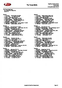
Figure 1: Real-Time Statechart Figure 1 depicts a (part of a) Real-Time Statechart, consisting of 2 states and 1 transition. The state S1 has the time invariant t0 ≤ 5msec, S2 ’s invariant is t0 ≤ 20msec ∧ t1 ≤ 13msec (t0 and t1 denote clocks). The transition is triggered by the event e, the guard [x ≤ 2] and by the time guard [1msec ≤ t0 ]. When firing t2 is reset and action(), which has the WCET w = 2msec, is executed. The firing of the transition has to be finished at the latest 10msec after being triggered and at t1 == 6. The earliest point in time, when S2 may be entered is at t1 == 3. Worst-case execution times are attached to the entry()-, exit()- and do()-operations, too, clock can be reset when entering and exiting the states, too. As the do()-operation is executed periodically, an interval is specified from where a fixed period is chosen. Giving a compact overview, Real-Time Statecharts offer the following constructs for states: Hi4 www.fujaba.de
6.2 Semantics
25
erarchy, parallelism, and time invariants. Transitions make use of the constructs: Events, guards, time guards, resets, priorities, and synchronization. It is shown, that they can be mapped to a corresponding ExHTA. The semantics of the Real-Time Statecharts is defined by these mapping rules.
6.2
Semantics
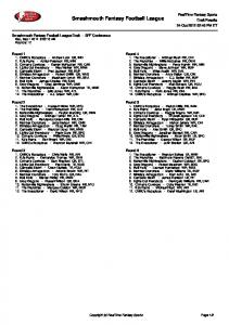
Before outlining the semantics by showing the mapping rules, we will introduce an abbreviation. Figure 2 a) shows an ExHTA with an urgent transition from location S1 to S2 and a non-urgent transition from S2 to S3 . S2 is a hierarchical state with the invariant t0 ≤ 10 and the substates S21 , S22 and S23 which have the same invariant (in this example); action1 () and action2 () are resets. Such a hierarchical state can be abbreviated as shown in Figure 2 b). There, the sequential executed resets action1 () and action2 () are combined to action() and the substates disappear.
Unit: msec a)
b)
S1
S1
t0 ≤ 2
t0 ≤ 2
[(5 ≤ t0 ≤ 10)∧ e [x < 2] (20 ≤ t1 ≤ 25)] {t1 }
[(5 ≤ t0 ≤ 10)∧ e [x < 2] (20 ≤ t1 ≤ 25)] {t1 }
S2
S2 S21 t0 ≤ 10
action1 () S22 t0 ≤ 10
action2 () S23 t0 ≤ 10
action() w=5
t0 ≤ 10
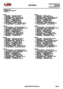
t0 ≤ 10 S3 t0 ≤ 10 S3 t0 ≤ 10 Figure 2: Extended Hierarchical Timed Automata Using this abbreviation, a Real-Time Statechart can be mapped to an ExHTA –as depicted in Figures 3 and 4. Figure 3 shows how non-hierarchical states are mapped to locations: The name as well as the invariant are held. The entry()- and exit()-operations and the sets of clockresets will be rolled out of the states. To modell the periodic execution of the do()-operation, a transition with its specific state as source and target will be created. This transition resets the new introduced clock tint and is only triggered at tint == p, where p ∈ [plow , pup ]. When firing a transition, the exit()-operation of the source state, the data assignment and the target state’s entry()-method are executed sequentially. This is modelled in the ExHTA by putting
26
6
REAL-TIME STATECHARTS
Extended Hierarchical Timed Automata
Realtime Statechart S1
S1
inv
{tint }
entry() CRentry do() p ∈ [plow ; pup ] exit() CRexit
inv
do() p ≤ tint ≤ p
Figure 3: Mapping of non-hierarchical states
Realtime Statechart e g
exitsrc
tg
/action()
wa
prio entrytgt
CR �
[dlow ; dup ]
i (ti
∈ [dilow ; diup ])
ExHTA S0 e g
tg
prio CR∪ {tint }∪ CRexitsrc
exitsrc () (d �low i≤ tint ≤ dupi)∧ action() i (dlow ≤ ti ≤ dup ) entrytgt () CR entrytgt wexitsrc + wa + wentrytgt (t �int ≤ dupi)∧ i (ti ≤ dup )
Figure 4: Mapping of transitions
6.3 Realizability
27
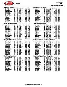
them in a hierarchical state –similar to Figure 2– and using the abbreviation, introduced above. This leads to 2 different kinds of locations: Statelocations, representing states and actionlocations in which operations are executed. The WCET of these 3 actions is the sum of their single WCETs. In Figure 4 is shown, that a transition is mapped to an actionlocation and 2 transitions (an urgent and a non-urgent one), connecting it with the source and the target state. The event, guard, timeguard and priority from the Real-Time Statechart is recovered in the urgent transition as these attributes shall trigger the actions. The deadline is recovered at multiple places. On the one hand it is used to extend the invariant of the actionlocation, on the other hand it is used to prevent the actionlocation to be left before it may be left, specified by the lower bound of the deadline. As the last point of time, when the actionlocation may be left, is specified by the upper bound of the deadline, it is used for the upper bound of the timeguard of the non-urgent transition. The constructs of parallelity, hierarchie and history can be adopted without changes, because Real-Time Statecharts offer them as well as ExHTA.
6.3
Realizability
To achieve a mapping from the model to real physical threads, deadlines and WCETs are required for every transition. These deadlines specify the point in time, when the execution has to be ended relative to the moment of triggering or relative to one or multiple clocks. Thus, the modeller has to respect, that the firing of a transition (respectively the execution of resets and data assignments) is not infinitely fast and needs time to be executed. Usually, the WCETs are dependant on the target platform. Note that the WCET of an operation needs to be less than its deadline. The timedifference between WCET and deadline respects that other tasks require resources simultaneously and that on real physical devices a triggered transition is usually recognized with a delay. This delay is compensated by that timedifference. Thus, the designation of WCETs and deadlines permits the mapping of the model to real physical threads that can be executed on a (limited) physical digital controller. These threads can be implemented in every programming language, supporting real-time functionality. The CASE-Tool Fujaba5 delivers an implementation of Real-Time Statecharts for Real-Time Java. When multiple Real-Time Statecharts are executed in parallel on the same processor, WCETs and deadlines are used to perform a schedulability analysis before code is generated. The specification of invariants, deadlines, guards and WCETs potentiates to model time inconsistencies, e.g. an invariant of a state expires before any transition, leaving from this state, is triggered. By analysing the structure of the Real-Time Statechart and the coherency of the temporal annotations, some conflicts and inconsistencies can be detected with an appropriate complexity (e.g. no state space exploration, usually caused by model checking tools). For cases where this analysis is not capable to determine whether a timing fault is present or not, model checking should be employed.
6.4
Summary
With the model of Real-Time Statecharts it is possible to specify complex behavior by the use of hierarchy and parallelism as well as temporal behavior. Additionally, it is possible to specify operations executed at the moment of entrance or exit of a state (entry()-/exit()-operation) or being periodically invoked during residence in a state (do()-operation). Real-Time Statecharts fulfill all requirements pointed out in Section 2 and ensure that only limited behavior is specified that is realizable. 5 www.fujaba.de
28
7
7 RELATED WORK
Related Work
Harel introduced in [Har98] 2 extensions of Statecharts to bring in time constraints: Using the timeout -construct an event e and a time t is associated with a transition. The transition is triggered t time-steps after the occurence of the event e. If a reset or data assignment is marked as scheduled action, it is not executed during firing a transition, but a specified time later (although the state is changed immediately). In [KP92] an extension is described, that allows to specify a kind of delay interval for a transition. The bounds of this interval define how much time elapses at least and at most between triggering and firing the transition. In [PAS94] a similar approach is used. There, the interval describes the points in time, when the source state can be left earliest and when it has to be left at the latest. In addition, every event obtains a duration, indicating how long it can be consumed after creation. All the constructs, described above, are useful to specify temporal behavior for unlimited systems. To map them on man made controllers, more informations are needed (e.g. WCETs, deadlines, etc.). In [SKW00] the model of an automaton is mapped to a so called multi-tasking model. The multitasking model describes how the actions of the model are placed in physical threads. The annotation of WCETs and deadlines in the model makes this mapping possible. The automaton offers communication via synchronous and asynchronous events. Compared to high-level automata, it is restricted, as it is not possible to use hierarchy, parallelism or to trigger transitions dependant on clocks or variables. [LQV01] deals with validation of real-time models. UML (in particular class-diagrams and extended Statecharts) is used to specify the structure and behavior, based on time. As no WCETs and deadlines are required and time comes in just by the use of the after-construct, the problems mentioned above, occure here, too. The claimed invariants of the system behavior are expressed by OCL constraints. The specified model can be translated into the first order temporal logic language TRIO, that can be used as input for the modelchecker TRIO-Matic in order to validate the properties of the model. To formalize the semantics of the extended Statechart model, it is mapped to an extension of Timed Statecharts in [BLM02]. In [LC96] Duration Calculus –an extended first order logic language– is used to extend Statecharts with duration. Thus, there exist a couple of functions determining if and for which time states are active within a specific timeinterval. This framework, expressing temporal requirements as functions, was regarded as breakthrough in validation of not only functional but also temporal correctness. Another approach for verifying real-time systems is given in [KMR02], where behavior is specified by UML Timed State Machines, that are mapped to Timed Automata, serving as input for the Modelchecker UPPAAL [DMY02]. Also in this work, it is assumed that the Timed State Machine runs on an unlimitted, infinite fast device. Anyhow, it is assumed, that the Statechart is distributed and it is possible to specify an upper bound for the delay of communication. In addition to the Timed State Machine, so called collaborations are specified by the use of sequence diagrams. These sequence diagrams are transformed to the UPPAAL conformant Observer Timed Automata. After that UPPAAL is used to verify the Timed Automaton against the Observer Timed Automaton. As model checking requires a formal semantics, that is not provided by UML, [EW00] delivers another formal semantics for Statecharts at the requirements-level, orientated at the StateMate semantics. In the paper, a comparison is given of structured and object oriented Statechart semantics as well as a comparison of Statecharts at the requirements- and at the implementation-level. The main aspect describes the communication between several Statecharts. All this work and the extensions are useful for verification and validation of systems, whose behavior is based on time. As none of the models have been designed with the aim of generating code, they do not provide solutions appearing in this domain.
29
8
Conclusion
For the proposed notion of Extended Hierarchical Timed Automata the required modeling notation properties expressiveness, temporal behavior and predictability follows from the extension of the hierarchical Timed Automata concepts. While the proposed extension of priorities limit at least the ability to employ model checking the resulting extended hierarchical state machines, integrating an arbitrary complex data, permit to even check an finite abstraction of real models. The presented formal extension of the hierarchical Timed Automata has been employed in order to define the semantics for Real-Time Statecharts [Bur02]. Each Real-Time Statechart is mapped to a limited Extended Hierarchical Timed Automaton which is bi-partite with respect to do and activity states. The realizability of consistent models of this limited notion of Extended Hierarchical Timed Automata has been shown in Section 6. The presented notion therefore supports all four identified requirements and thus better serves the required modeling of complex reactive real-time systems.
Acknowledgements The authors thank Martin Hirsch and Matthias Meyer for comments on earlier versions of the report.
References [ACD90]
Rajeev Alur, Costas Courcoubetis, and David Dill. Model-checking for Real-Time Systems. In Proc. of Logic in Computer Science, pages 414–425. IEEE Press, June 1990.
[AD90]
Rajeev Alur and David Dill. Automata for Modelling Real-Time Systems. In Proc. of the International Colloquium on Algorithms, Languages and Programming, volume 443 of Lecture Notes in Computer Science, pages 322–335. Springer Verlag, July 1990.
[AD94]
Rajeev Alur and David L. Dill. A Theory of Timed Automata. Theoretical Computer Science, 126:183–235, 1994.
[AK96]
R. Alur and R. P. Kurshan. Timing Analysis in COSPAN. In R. Alur, T. A. Heizinger, and E. D. Sontag, editors, Hybrid Systems III, volume 1066 of Lecture Notes in Computer Science, pages 220–231. Springer Verlag, 1996.
[BD00]
B´eatrice B´erard and Catherine Dufourd. Timed automata and additive clock constraints. Information Processing Letters, 75(1-2):1–7, July 2000.
[BLL+ 95]
Johan Bengtsson, Kim G. Larsen, Fredrik Larsson, Paul Pettersson, and Wang Yi. Uppaal — a Tool Suite for Automatic Verification of Real–Time Systems. In Proc. of Workshop on Verification and Control of Hybrid Systems III, number 1066 in Lecture Notes in Computer Science, pages 232–243. Springer–Verlag, October 1995.
[BLM02]
V. Del Bianco, L. Lavazza, and M. Mauri. A Formalization of UML Statecharts for Real-Time Software Modelling. 2002.
[BR99]
Loic P. Briand and Daniel M. Roy. Meeting Deadlines in Hard Real-Time Systems: The Rate Monotonic Approach. IEEE Press, 1999.
30
REFERENCES
[Bro86]
Manfred Broy. A theory of nondeterminism, parallelism, communication and concurrency. Theoretical Computer Science, 45, 1986.
[B¨ uc62]
J. R. B¨ uchi. On a decission method in restricted second order arithmetic. In Proc. of the 1960 Int. Congt. on Logic, Methodology and Philosophy of Science, pages 1–11. Stanford University Press, 1962.
[Bur02]
Sven Burmester. Generierung von Java Real-Time Code f¨ ur zeitbehaftete UML Modelle. 2002.
[BW01]
Alan Burns and Andy Wellings. Real-Timer Systems and Programming Languages: Ada 95, Real-Time Java and Real-Time POSIX. Addison-Wesley, 3rd edition, 2001.
[DH94]
D. Drusinsky and D. Harel. On the Power of Bounded Concurrency I: Finite Automata. Journal of the ACM, 41(3), 1994.
[DMY02]
Alexandre David, Oliver M¨ oller, and Wang Yi. Formal Verification of UML Statecharts with Real-time Extensions. In Ralf-Detler Kutsche and Herbert Weber, editors, Proceedings of FASE 2002, number 2306 in Lecture Notes in Computer Science, pages 218–232. Springer Verlag, 2002.
[DOTY96]
C. Daws, A. Oliverio, S. Tripakis, and S. Yovine. The Tool KRONOS. In R. Alur, T. A. Heizinger, and E. D. Sontag, editors, Hybrid Systems III, volume 1066 of Lecture Notes in Computer Science, pages 208–219. Springer Verlag, 1996.
[DY95]
C. Daws and S. Yovine. Two examples of verification of multirat timed automata with KRONOS. In Proc. of the 16th IEEE Real-Time Symposium. IEEE Press, December 1995.
[EMSS90]
E. A. Emerson, A. K. Mok, A. P. Sistla, and J. Srinivasan. Quantitative temporal reasoning. In Proceedings of the Second Workshop on Computer-Aided Verification, volume 531 of Lecture Notes in Computer Science, pages 136–145, 1990.
[EW00]
R. Eshuis and R. Wieringa. Requirements-level semantics for uml statecharts. In S.F. Smith and C.L. Talcott, editors, Formal Methods for Open Object-Based Distributed Systems IV (FMOODS 2000), pages 121 140. Kluwer Academic Publishers. Kluwer Academic Publishers, 2000.
[Har87]
D. Harel. STATECHARTS: A Visual Formalism for complex systems. Science of Computer Programming, 3(8):231–274, 1987.
[Har98]
D. Harel. Modeling reactive systems with statecharts. McGraw-Hill, 1998.
[HHWT95a] T. A. Heizinger, P.-H. Ho, and H. Wong-Tai. A Userguide to HYTECH. In E. Brinksma, W. R. Cleaveland, K. G. Larsen, T. Margaria, and B. Steffen, editors, Tools and Algortihms for the Construction and Analysis of Systems, volume 1019 of Lecture Notes in Computer Science, pages 41–71. Springer Verlag, 1995. [HHWT95b] Thomas A. Henzinger, P.-H. Ho, and H. Wong-Toi. HyTech: The Next Generation. In Proc. of the 16th IEEE Real-Time Symposium. IEEE Press, December 1995. [HNSY92]
Thomas A. Henzinger, Xavier Nicollin, Joseph Sifakis, and Sergio Yovine. Symbolic Model Checking for Real-Time Systems. In Proc. of IEEE Symposium on Logic in Computer Science. IEEE Press, 1992.
[HU79]
John E. Hopcroft and Jeffrey D. Ullman. Introduction to Automata Theory, Languages and Computation. Series in Computer Science. Addison-Wesley, Reading, MA, USA, 1979.
REFERENCES
31
[Jos96]
Mathai Joseph. Real time systems : specification verification and analysis. Prentice Hall international series in computer science. Prentice Hall, 1996.
[KMR02]
A. Knapp, S. Merz, and C. Rauh. Model Checking timed UML State Machines and Collaborations. 7th International Symposium on Formal Techniques in Real-Time and Fault Tolerant Systems (FTRTFT 2002), Oldenburg, September 2002, Lecture Notes in Computer Science volume 2469 pages 395-414. Springer-Verlag, 2002.
[KP92]
Y. Kesten and A. Pnueli. Timed and Hybrid Statecharts and their Textual Representation. In J. Vytopil, editor, Formal Techniques in Real-Time and Fault-Tolerant Systems, volume 571 of Lecture Notes in Computer Science. Springer Verlag, 1992.
[Lam77]
Leslie Lamport. Proving the correctness of multiprocess programs. IEEE Transactions on Software Engineering, 3(2):125–143, March 1977.
[LC96]
K. Leung and D. Chan. Extending Statecharts with Duration. In 20th International Computer Software Applications Conference, volume 2306 of IEEE Press, 1996.
[LPY95]
Kim G. Larsen, Paul Pettersson, and Wang Yi. Compositional and Symbolic ModelChecking of Real-Time Systems. In Proc. of the 16th IEEE Real-Time Systems Symposium, pages 76–87. IEEE Computer Society Press, December 1995.
[LPY97]
K. Larsen, P. Pettersson, and W. Yi. UPPAAL in a Nutshell. Springer International Journal of Software Tools for Technology, 1(1), 1997.
[LQV01]
L. Lavazza, G. Quaroni, and M. Venturelli. Combining UML and Formal Notations for Modelling Real-Time Systems. In Joint 8th European Software Engineering Conference (ESEC) and 9th ACM SIGSOFT International Symposium on the Foundations of Software Engineering (FSE), Vienna Austria, September 2001.
[LS01]
G. Logothetis and K. Schneider. Symbolic Model Checking of Real-Time Systems. In International Symposium on Temporal Representation and Reasoning, pages 214– 223, Cividale del Friuli, Italy, June 2001.
[Mil89]
R. Milner. Communication and Concurrency. Prentice-Hall International, 1989.
[Obj01]
Object Management Group. OMG Unified Modeling Language Specification, Version 1.4, September 2001. OMG document ad/01-09-67.
[PAS94]
A. Peron and A.Maggiolo-Schettini. Transitions as Interrupts: A New Semantics for Timed Statecharts. In Proceedings of TACS ’94, volume 789 of Lecture Notes in Computer Science. Springer Verlag, 1994.
[Pet99]
Paul Pettersson. Modelling and Verification of Real-Time Systems Using Timed Automata: Theory and Practice. Unpublished, Department of Computer Science, Uppsala University, Denmark, February 1999.
[PL00]
Paul Pettersson and Kim G. Larsen. Uppaal2k. Bulletin of the European Association for Theoretical Computer Science, 70:40–44, February 2000.
[Pnu77]
Amir Pnueli. The temporal logic of programs. In 18th Annual Symposium on the Foundations of Computer Science, pages 46–57. IEEE Press, November 1977.
[Pur99]
Anuj Puri. An Undecidable Problem for Timed Automata. Discrete Event Dynamic Systems, 9(2), May 1999.
[RK99]
J. Ruf and T. Kropf. Modeling Real-Time Systems with I/O-Interval Structures. In GI/ITG/GMM Workshop Methoden und Beschreibungssprachen zur Modellierung und Verifikation von Schaltungen und Systemen, pages 91–100. Shaker Verlag, March 1999.
32
REFERENCES
[RK00]
J. Ruf and T. Kropf. Analyzing Real-Time Systems. In Design, Automation and Test in Europ (DATE), Paris France, March 2000. IEEE Computer Press.
[SKW00]
M. Saksena, P. Karvelas, and Y. Wang. Automatic Synthesis of Multi-Tasking Implementations from Real-Time Object-Oriented Models. In Proceedings of the Third IEEE International Symposium on Object-Oriented Real-Time Distributed Computing, Newport Beach, California, 2000.
[WM97]
Michal Walicki and Sigurd Meldal. Algebraic Approaches to Nondeterminism—an Overview. ACM Computing Surveys, 29(1):30–81, March 1997.