Realization of A Generalized Modeling Method for Ungrounded Power Systems in Matlab/Simulink Li Qi,
*
Karen L. Butler-Purry, Stephen Woodruff *
Center for Advanced Power Systems Florida State University, Tallahassee, FL 32310
[email protected]
Electrical Engineering Department Texas A&M University College Station, TX 77843 short lines are very large in ungrounded systems, which reduced the speed of the detailed simulations [3]. The simulation speed is improved greatly by neglecting the strayed capacitances, which have negligible effects on stability study. Without the shunt capacitors, ungrounded systems are completely isolated from ground and inductor buses, where only inductive components are connected, emerge in ungrounded systems. The nodal admittance matrix based modeling methods, such as EMTP/ATP [4], are no more applicable because of the singularity of the admittance matrix. Equation based modeling methods, such as SimPowerSystems [5], does not allow connecting inductive synchronous generators in series with inductive lines since incompatible interconnection of only voltage-in current-out inductive models on inductor buses. The bus voltages of inductor busses need to be established by artificial ways, such as paralleling an auxiliary resistor [5]. A generalized strategy for modeling ungrounded finite inertia power systems was developed by the authors to simulate ungrounded power systems [6]. This generalized modeling method is based on reformulated voltage-in fluxout reference generator model and voltage-current-in voltage-out line models. Keeping the original physical model of a component, reformulated models changes only the standard mathematical representation of the component model. Bus voltages can be calculated from a set of algebraic equations at each inductor bus. Once bus voltages are derived, the other variables in the modeled system are solved. This generalized method was compared with two other modeling methods for SPS [3][7] in [6]. This paper is concentrated on the realization of the generalized modeling method in Matlab/Simulink. This realization is verified by simulation results of ungrounded systems in Matlab/Simulink. In section 2, component models are developed with existing function blocks. The interconnected with algebraic loops of the generalized method in Matlab/Simulink is compared with the interconnection of the method in [7]. Construction of a system model in Matlab/Simulink is illustrated in section 3. In section 4, representative simulation results and speed of various types of faults in a reduced ring SPS modeled in Matlab/Simulink are presented. In section 5, results of the generalized modeling method and SimPowerSystems are compared. Some conclusions are drawn in section 6.
Keywords: Matlab/Simulink, nonlinear, ungrounded Power Systems, building blocks, algebraic loops. Abstract Matlab/Simulink provides a customized environment to realize a generalized modeling method previously developed by the authors for ungrounded power systems. Problems of building component models with function blocks and interconnecting them with algebraic loops in Matlab/Simulink are discussed. The system model of a reduced ring shipboard power system is built in Matlab/Simulink according to the model construction procedures. Representative simulation results of various fault scenarios of the reduced system are presented. Comparison of simulation results and speeds of the generalized modeling method and a commercial software package SimPowerSystems, which was developed in Matlab/Simulink, validates the effectiveness of the implementation of the generalized modeling method in Matlab/Simulink. 1.
INTRODUCTION Power systems are nonlinear systems. Due to the large amount of nonlinearity of power system components, modeling and simulation of power systems are challenging. Shipboard power systems (SPS) in U.S naval ships supply electric power to weapon, navigation, communication and operation systems on naval ships. AC radial SPS found currently on US surface combatant ships is a typical ungrounded power system [1]. In ungrounded power systems, no equipment is intentionally connected to ground, the inertia of generators is finite, and the distance between equipment is short. Dynamic simulations provide valuable information for power system stability study of ungrounded power systems. Salient features of ungrounded power systems require special consideration on the modeling of shipboard power systems [2]. Due to the finite inertia generators and stiff connections between components, detailed component models, such as high order machine models, should be used for dynamic simulations [1]. However, due to the small strayed capacitances of cables, the natural frequencies of
SCSC 2007
37
ISBN # 1-56555-316-0
i0 = lls −1λ0
2.
COMPONENT MODELS AND INTERCONNECTION IN MATLAB/SIMULINK Any power system component can be modeled by a set of nonlinear differential-algebraic-equations (DAE) in the form of (1),
(7)
•
1 (TM − TE ) 2H TE = λ d i q − λ q i d
ωr = where R 1 =
•
(1) x = f (x,u, t ) Matlab/Simulink is a powerful software package for modeling, simulating, and analyzing dynamical systems by building models as block diagrams with a graphical user interface (GUI) [8]. Having many features to allow customization, Matlab/Simulink can simulate dynamic systems by solving user-defined Differential-Algebraic Equations (DAE) with given integration rules [8]. The construction of these models and the interconnection in Matlab/Simulink are described in this section.
[
λ Dq = λ D
diag (rs ,−rkq' )
λq
, R2 =
]T , λ Qdf = [λQ
λd
(8) (9)
diag ( rs ,− rkd' ,− r f' λf
]T .
),
T1 and T2 are two
constant vectors. T1=[1 0] , and T2=[1 0 0]T. Vectors λ Qq , i Qq , u Qq are in the form of f Dq = f D f q T , T
and λ Ddf , i Ddf , u Ddf are in the form of f Ddf = [ f D ⎡− lls − l ' lkq L1 = ⎢ ⎢⎣ l mq
⎡− lls − l '
lkd ⎢ l mq ⎤ , L l = − ⎥ ⎢ 2 md ' lls + l lkq ⎥⎦ ⎢ ⎢ − l md
l md l s + l lfd '
l md
⎣
[
]
fd
]T .
ff
l md ⎤ ⎥ l md ⎥ . ' ⎥ l s + l lkd ⎥⎦
Scalar rs is the resistance of each stator windings r fd' , rkq' ,
2.1. Component Models in Matlab/Simulink Matlab/Simulink includes an extensive library of predefined blocks to build graphical models of the dynamical systems using drag-and-drop operations. A library for component models of ungrounded power systems was developed in Matlab/Simulink for the generalized modeling method. The mathematical representation of each component model was discussed in detail by the authors [6]. Each component model in the library is a customized subsystem. It was built with a comprehensive set of predefined Matlab/Simulink blocks with functions, such as integration, sum, product, and switch, to represent mathematical equations of the component model. Two reformulated component models, the reference generator model, which is selected as the largest generator in a system, and the reformulated cable model, are essential component models in the generalized modeling method and will be discussed in this section. The reformulated models are developed from standard component models [9] and solve the interconnection incompatibility at inductor buses. The reference generator model, shown as (2)-(9), is reformulated from the standard generator model to facilitate the derivation of the reference generator bus voltages. Instead of currents in standard generator model, flux linkages are the state variables and outputs of the reference generator model.
rkd' are the resistances and leakage inductances of rotor
windings. ω r is the angular speed of the rotor. lls is the ' ' leakage inductance of each stator windings, and llkq , llfd ,
' llkd are the leakage inductances of rotor windings, lmq and lmd are the magnetizing inductances on q- and d-axis. The reformulated line model, shown as (10), is reformulated from the standard line model to calculate the input voltages of the inductor bus. Instead of voltage difference as inputs and currents as outputs, the reformulated cable model has sending end voltages and currents as inputs and receiving end voltages as outputs.
u r = u s − (PRP −1 + PL
where u r
[
= ur0
u rd
u rq
• dP −1 )i − PLP −1 i dt
]T , u s = [u s0
u sd
u sq
(10)
]T , i = [i r
0
id
iq
]T .
λ0 = − rr i0 + u 0
(4)
Subscripts s and r denote the variables associated with the sending and receiving ends of lines. The matrices R and L include self and mutual resistances and inductances of threephase lines. Each component model is a mask subsystem in Simulink. Parameters of components are user-defined on masks. The structure of a component model, including the function blocks and their connections, is revealed after the mask subsystem is opened. Figure 1 illustrates the realization of (2) and (5) in Matlab/Simulink. Equations (2) and (5) are used to calculate variables on quadrate axis in a reformulated generator model. In Figure 1, equation (2) is built by the blocks, including “product” and “sum”, within the dashed rectangle. Function blocks “Integral” are used to
i Qq = L 1 −1 λ Qq
(5)
derive λQ and λ q from their derivatives λQ and λq . The
i Dfd = L 2 −1 λ Dfd
(6)
•
λ Qq = R 1 i Qq + ω r T1 λ Dq + u Qq •
λ Ddf = R 2 i Ddf − ω r T2 λ Qdf + u Ddf •
ISBN # 1-56555-316-0
(2) (3)
•
•
inputs λD and ωr are derived from (3) and (8), respectively, and used as inputs of (2). Outputs iq and iQ from (5) are fed back into the calculation of (2) as inputs. The other
38
SCSC 2007
component models are built with existing function blocks in Matlab/Simulink in the same way as shown in Figure 1. ωr
•
uQ
λD
λQ ×
+
∫
λQ
(5)
iQ
×
rs
(2)
in modeling ungrounded power systems. When a model contains an algebraic loop, Matlab/Simulink calls a loop solving routine at each time step [8]. This Simulink loop solver uses Newton’s method with weak line search and rank-one updates to a Jacobian matrix of partial derivatives and calculates algebraic variable in each algebraic loop. In the generalized modeling method, bus voltages of ungrounded power systems thus are solved from the algebraic loops formed by the component models and the algebraic equations (10)-(12). In a SPS modeling method by Ciezki [7], forced linear combinations of weighted summations of currents and current derivatives are used to form algebraic constraints [7]. The weights are selected manually to derive desirable simulation performance. In the generalized method, algebraic loops are naturally formed by component models and interconnection equations. The coefficients of mathematical equations are accounted for the weights of the algebraic loops. This natural formation of algebraic loops saves the trouble of manual selection of appropriate weights to compromise simulation speed and simulation performance. It must be noted that, with the size of a system enlarged, the number and complexity of algebraic loops increased, which may decrease execution speed of the generalized modeling method in Matlab/Simulink.
iq
uq
' − rkq
+
• λq
×
∫
λq
Figure 1 Modeling of Equations (2) &(5) in Matlab/Simulink
2.2. Component Interconnection in Matlab/Simulink As described earlier, component models should be connected at inductor buses by artificial ways. Kirchoff’s Current Law (KCL), shown as (11), is used on each bus to derive unknown currents. With the flux linkages from the reference generator (2)(3) and the generator current calculated from (11), the reference generator voltages are derived by (12). The bus voltages of the other inductor buses in ungrounded systems are calculated by the reformulated cable model (10). The interconnections on the reference generator buses and other inductor buses in ungrounded power systems are shown in Figures 1 and 2 by the authors [6].
3.
MODELING OF A REDUCED SHIPBOARD POWER SYSTEM IN MATLAB/SIMULINK A reduced ring configured SPS is shown in Figure 2. It is used to illustrate the construction of the system model with the generalized modeling method in Matlab/Simulink. More examples of ungrounded SPS models in Matlab/Simulink can be found in [10]. In the reduced system, generators 1 and 2 are running at normal operating condition, while generator 3 is a back up generator. Three generator switchboards are connected in a ring with cables to provide more flexibility of system configuration. This reduced SPS has four busses: generator switchboards 1, 2, 3, and load center 5. Load center 5 is connected downstream of switchboard 2 and upstream of three-phase transformer 1. The transformer is in turn connected upstream of unbalanced static load 5. To model an ungrounded system, first, component models are selected from the component model library developed in Matlab/Simulink. At second step, the system model of an ungrounded system is formed by connecting various component models, which includes interconnection equations (11)(12). Finally, simulation parameters, including time step and integration algorithm, are selected by in “parameter configuration”.
K
∑i
k
=0
(11)
k =1
•
v = −rs i − λ + P
dP −1 λ dt
(12)
where i k = [ik 0 ikd ikq ]T . k denotes the current associated with the kth branch connected to the bus. rs = diag (rs rs rs ) . Since component models are interconnected at inductor buses to form an ungrounded power system, some input variables may be indirectly connected to the output variables by feedback paths through blocks used in the system. For example, in Figure 1, since the outputs iq and iQ of (5) are feedback as inputs of (2), inputs of (2) and (5) are indirectly connected with outputs of (2) and (5). In Simulink, an algebraic loop generally occurs when an input port with direct feedthrough is driven by the output of the same block, either directly, or by a feedback path through other blocks with direct feedthrough [8]. With the generalized modeling method [6], algebraic loops thus occur
SCSC 2007
39
ISBN # 1-56555-316-0
cables 12 and 23. The currents of cables 12 and 23 modeled by the reformulated cable model, and all loads downstream of switchboard 1 are summed and taken as the current summation inputs of the interconnection equations on the reference generator bus, which is generator switchboard 1. Therefore, the outputs of the interconnection equation (12) are the voltages on generator switchboard 1. In summary, component models of ungrounded power systems are built as subsystems using function blocks in Matlab/Simulink. The interconnection of component models forms algebraic loops in Matlab/Simulink. The input voltages of all component models are either the reference generator bus voltages or bus voltages calculated with (10) or (12). After these bus voltages are solved by the given algebraic solver of Matlab/Simulink, a ungrounded power system can be simulated.
Generator Motor
1 1
Static load Load center Cable Switchboard Transformer 2
1 12
1
13 3 23
2 2
3 3
5
3 1
25
5 5
Figure 2 Single Line Diagram of A Reduced Ring SPS
Fig 4 presents a diagram to illustrate the structure of the system model for the reduced ring SPS in Fig 3 in Matlab/Simulink. Generator 1 is selected as the reference generator. The output currents of load models downstream of load centers are summed and input into the KCL equations of the load centers. The output currents of the KCL equations of the load centers are the currents of the cables upstream of the load centers, which are then fed into the KCL equations of upstream generator switchboards. The output currents of the KCL equations of the switchboards are the currents of tie line cables between switchboards 1,2 and 2,3. Cable 13 adopts the standard cable model and its current outputs are used to derive the current inputs of flux1
Generator 1
Inter connection
4.
DYNAMIC SIMULATIONS IN MATLAB/SIMULINK To illustrate the effectiveness of the system model constructed in previous section, various faults are simulated in the reduced ring SPS in the environment of Matlab/Simulink. The selected integration algorithm is Dormand-Prince ODE5 with a fixed time step of 0.001. The error tolerance of the integration algorithm is selected by the algorithm automatically. The parameters of the components of the example system are listed in Appendix. Motors in the system use M4 in the Appendix. Unless specified, these parameters are in per unit with Vbase=450V (rms, line-toline) and Sbase=3.125MVA.
v1
Cable13
v3
Generator 3
v3
ig1 KCL1
Static load 1
v3
i13
Motor3
Motor1 v6
KCL3
i36
il3,im3
ig3
Static load3 il6,im6
i23
Cable23 v2
Cable12
Generator 2 v2
i12
v2
Static load2
KCL2
ig2 Motor2
Figure 3 Construction of System Model in Matlab/Simulink
ISBN # 1-56555-316-0
40
SCSC 2007
the generalized modeling method on the reduced ring SPS in Matlab/Simulink. In an attempt to evaluate the simulation speed of the generalized modeling method of the test system shown in Figure 2 in Matlab/Simulink, 50 runs of phase A to ground faults are executed on the reduced ring SPS. Simulations of other fault scenarios take similar CPU time. These runs were executed in Matlab/Simulink 6.3 on a Pentium PC, whose clock speed is 2.66 GHZ. Identical results were observed from the 50 runs. Among the 50 runs, the maximum CPU time of a single run is 419.56 seconds, and the minimum time was 416.11 seconds. The average CPU execution time of the 50 runs was calculated and considered as the CPU time of the generalized modeling method. With this average execution time, a six second simulation of the reduced shipboard power system requires CPU execution time of approximate 419 seconds.
In this paper, the system is initially running at steady state condition. Figure 4 in [6] shows the steady state simulation results after the initially disconnected loads in the system of Figure 2 are energized at one second. A fault then begins at 0.5s and lasts for 0.5s. The fault location is in front of static load 5 and after the linear transformer 1. Four faults, including single-phase-to-ground, two-phase, twophase-to-ground, and three-phase-to-ground faults, are simulated in the system. They are: (1) Phase A to Ground Fault; (2) Phase A and B Fault; (3) Phase A and B to Ground Fault; and (4) Three-Phase-to-Ground Fault. Here, the ground is referred to ship hull, which is considered remotely connected to ground with water. Figure 4 shows the three phase line-to-line voltages of the four faults at fault location. For delta connected power system, line-to-line voltages are important variables to evaluate system operation. For single-phase-to-ground faults, since the rest part of the system is ungrounded, no fault current should flow through the system and normal system operation should not be affected. In Figure 4(a), the line-to-line voltages during the fault keep the same values as at pre-fault condition, which agrees with the previous analysis of no effects on system operation during singlephase-to-ground faults. Figure 4(b) and 4(c) show similar line-to-line voltages, which indicate two-phase and twophase-to-ground faults have similar effects on ungrounded system operation. In Figure 4(d), the line-to-line voltages decrease to zero after the three-phase-to-ground fault occurs. The line-to-line voltages shown in Figure 4 are as expected. The simulation results in Figure 4 testify the generalized modeling method and verify the realization of
5.
PERFORMANCE COMPARISON OF DIFFERENCE MODELING METHODS SimPowerSystems is a commercial power system simulation package developed by Hydro-Quebec in Matlab/Simulink. As described in section 1, by paralleling an auxiliary resistor with a generator, ungrounded power systems can be modeled by SimPowerSystems [5]. With a SPS simulated by the generalized modeling method and SimPowerSystems in Matlab/Simulink, simulation results from both methods are compared to validate the effectiveness of realizing the generalized modeling method in Matlab/Simulink.
1
1 AB BC CA
0.5 Line Voltage (p.u.)
Line Voltage (p.u.)
0.5
0
-0.5
-1
0.46
0.48
0.5 0.52 Time (Second)
AB BC CA
0
-0.5
-1
0.54
0.46
(a) Phase A to Ground Fault
0.54
1 AB BC CA
0
-0.5
0.46
0.48
0.5 0.52 Time (Second)
AB BC CA
0.5 Line Voltage (p.u.)
0.5 Line Voltage (p.u.)
0.5 0.52 Time (Second)
(b) Phase A, B Fault
1
-1
0.48
0
-0.5
-1
0.54
0.46
0.48
0.5 0.52 Time (Second)
0.54
(c) Phase A, B to Ground Fault (d) Three-Phase to Ground Fault Figure 4 Simulated Line-to-Line Voltages of the System Shown in Figure 2
SCSC 2007
41
ISBN # 1-56555-316-0
A portion of the power distribution system of a DDG-51 Navy destroyer, is shown in Figure 5. This reduced distribution power system was also used as example systems in [3][7]. In the system, one generator G1 is connected to three induction motors M1, M2, and M3 through a connecting cable. The load torque for each induction motor is square of its rotor speed, which represents a kind of speed-squared load. The parameters of this system can be found in Appendix and also in [3][7]. 1
Generator Motor Load center Cable Switchboard
G1
In addition to the comparison of the simulation results, simulation speeds of the generalized modeling method and SimPowerSystems are also compared. Table 1 shows the CPU execution time of the generalized method and the SimPowerSystems on the test system shown in Figure 5. 1000 runs were executed on the reduced SPS by the new modeling method and SimPowerSystems. Identical simulation results and close simulation speeds were observed from all runs. The average CPU execution time of the 1000 runs is calculated and considered as the CPU time. It is found from Table 1 that the simulation speed of the generalized method is much faster than of SimPowerSystems. In this paper, the generalized modeling method is realized from Matlab/Simulink. SimPowerSystems is developed in Matlab/Simulink [5]. In both methods, function blocks and integration algorithms are customized in building ungrounded system models. The simulation results from the two methods are similar. The generalized modeling method is much faster than SimPowerSystems in simulating the reduced distribution system in Figure 5. Natural formation of algebraic loops may contribute to the fast simulations of the generalized modeling method. The results presented in Figure 6 and Table 1 further verify the effectiveness of the Matlab/Simulink realization of the generalized modeling method.
1 1
M1 M2 M3
Figure 5 Single Line Diagram of A Reduced Distribution SPS
The system model of the system shown in Figure 5 is constructed in Matlab/Simulink according to the procedures of system model construction described in section 2. Since inductive components cannot be connected in series in SimPowerSystems, large auxiliary resistors of 0.1M Ω , are paralleled with the source and motor loads in the reduced distribution system. It is noted the size of the auxiliary resistor should be selected in order to achieve a good trade off between simulation speed and accuracy. The system is simulated using the generalized modeling method and SimPowerSystems in Matlab/Simulink 6.3 on the PC described in previous section. Some representative simulation results from the generalized modeling method and SimPowerSystems are shown in Figure 6. The simulations last five seconds. The generator is first operated at no load condition and then the induction motors are connected at 0.5 second. The generator terminal voltage and frequency drop as the induction motors started. The voltage controller and governor then react to the voltage and frequency drop and restore the terminal voltage and frequency back to their nominal values. In comparison of the simulation results from the generalized method and SimPowerSystems, high spikes are found in the results from SimPowerSystems. Since the load level in the system is not high, the ratio of the currents flowing through the shunt resistance and the motors to is not as high as that of the systems when the load level is high. This relatively low ratio may contribute to the high peak during start-up transient from SimPowerSystems. Selecting even larger shunt resistance may reduce the peak level of the transients. However, simulation speed is greatly reduced if the auxiliary resistance is high than 0.1M Ω .
ISBN # 1-56555-316-0
Table 1 CPU Execution Time of A Reduced Distribution SPS Simulation CPU Time Method Environment (CPU Type) SimPowerSystems Simulink 339.0781 seconds Generalized Method Simulink 2.0433 seconds
CONCLUSION The salient features of ungrounded power systems contribute to the creation of the generalized modeling method [6]. In this paper, the realization of system models with the generalized modeling method in the environment of Matlab/Simulink is discussed. Matlab/Simulink allows the customized construction and interconnection of component models. With the help of the Matlab/Simulink algebraic solver, bus voltages, which are the key of solving ungrounded power systems, are calculated. The system model of a reduced ring SPS is constructed and various faults are simulated in Matlab/Simulink. Simulations of a reduced distribution SPS by the generalized modeling method and the commercially available power system simulation package SimPowerSystems are also presented. The simulation results in sections 4 and 5 not only validate the generalized modeling method but also verify the effectiveness of the realization of the generalized modeling method in Matlab/Simulink.
6.
42
SCSC 2007
1.1
1.05
1.05
1
1
Vt (p.u.)
Vt (p.u.)
1.1
0.95 0.9
0.95 0.9
0.85
0.85
0.8
0.8
0.75
0.75
0
1
2
3
4
5
0
1
Time (Second)
2
3
4
5
4
5
4
5
Time (Second)
(a) Generator Terminal Voltage 1.005
W (p.u.)
W (p.u.)
1.005
1
0.995 0
1
2
3
4
1
0.995
5
0
1
Time (Second)
2
3
Time (Second)
0
-0.05
-0.05
-0.1
-0.1
T (p.u.)
T (p.u.)
(b) Generator Speed 0
-0.15
m
m
-0.15 -0.2
-0.2
-0.25
-0.25
-0.3
-0.3
0
1
2
3
4
-0.35
5
0
1
Time (Second)
2
3
Time (Second)
1
0.8
0.8
0.6
M1
W
1
WM1 (p.u.)
(p.u.)
(c) Generator Prime Mover Torque
0.4 0.2 0 0
0.6 0.4 0.2
1
2
3
4
0 0
5
Time (Second)
1
2 3 Time (Second)
4
5
(d) Rotor Speed of M3 Figure 6 Comparison of Simulation Results (1st column: the Generalized Modeling Method; 2nd column: SimPowerSystems)
References [1] K. L. Butler, N.D. R. Sarma, C. Whitcomb, H. D. Carmo, H. Zhang, “Shipboard Systems Deploy Automated Protection”, IEEE Computer Application on Power System, April 1998, pp.31-36. [2] L. Qi and K. L. Butler, “Analysis of Stability Issues during Reconfiguration of Shipboard Power Systems”,
7.
ACKNOWLEDGEMENT This work was sponsored in part by the Office of Naval Research, USA under Grant N00014-99-1-0704 at Texas A&M University.
SCSC 2007
43
ISBN # 1-56555-316-0
in Proc. 2005 IEEE PES General Meeting, San Francisco, CA, June 2005 [3] J. S. Mayer, O.Wasynczuk, “An Efficient Method of Simulating Stiffly Connected Power Systems With Stator and Network Transient Included”, IEEE Trans on Power Systems, Vol. 6, No. 3, August 1991, pp.922929. [4] H. Dommel, Electromagnetic Transients Program Reference Manual (EMTP Theory Book), 1986. [5] Hydro-Quebec TransEnergie, SimPowerSystems For Use With Simulink, Online only, The Mathworks Inc, July 2002. [6] L. Qi and K. L. Butler-Purry, “Reformulated Model Based Modeling and Simulation of Ungrounded Stiffly Connected Power Systems”, in Proc. 2003 IEEE Power Engineering Society General Meeting, Toronto, ON, July 2003. [7] J.G.Ciezki, R. W. Ashton, "The Resolution of Algebraic Loops In The Simulation of Finite-Inertia Power Systems", Proceedings of the 1998 IEEE International Symposium on Circuits and Systems, Vol. 3, pp.342-345. [8] Mathworks, Simulink – Dynamic System Simulation for Matlab, The Mathworks Inc, November 2000. [9] P. C. Krause, Analysis of Electric Machine, McGrawHill Series in Electrical Engineering, McGraw-Hill, New York, 1986. [10] L. Qi, Stability Analysis and Assessment for AC Shipboard Power Systems, Ph.D. Dissertation, Texas A&M University, College Station, TX. December, 2004.
KC=22.5, TC=0.55, TFV=0.01, TFT=0.05, WF10S=0.23, C2GT=0.251, C1GT=1.3523, CGNGT=0.5, WMAX=1.0, WMIN=0. 4. Induction motors (M1, IM2 and M3 [3][7]) Vbase=440V(rms, line-to-line), Pbase=150hp, M1: H=1.524, rs=0.0051, lls=0.00553, lm=2.678, l’lr=0.0553, r’r=0.0165. M2: Ubase=440V(rms, line-to-line), Pbase=40hp, H=1.054, rs=0.005, lls=0.0587, lm=2.952, l’lr=0.0587, r’r=0.0165. M3: Ubase=440V(rms, line-to-line), Pbase=200hp, H=0.992, rs=0.01, lls=0.0655, lm=3.225, l’lr=0.0655, r’r=0.0261. M4: Ubase=440V(rms, line-to-line), Pbase=192.6KW, H=0.98, rs=0.0198, lls=0.06, lm=2.7963, l’lr=0.0531, r’r=0.0529. 5. Cables Raa=Rbb=Rcc= 0.0205, Rab=Rbc=Rca= 0.005478, Laa=Lbb=Lcc= 0.169, Lab=Lbc=Lca = 0.1607. 6. Linear transformers N=450/120, R1= 0.3477, L1= 0.002478, R2= 0.024691, L2= 1.25 × 10 −7 , Lm= 24.91. 7. Static loads L1: Raa=Rbb=Rcc = 10; L3: Raa=Rbb=Rcc = 8, Laa=Lbb=Lcc = 6; L5: Raa= Rcc = 10, Rbb =20.
Appendix 1. Generators [1] rs=0.00515, r’kq=0.0613, r’fd=0.0011, r’kd=0.02397, lls=0.08, l’lkq=0.3298, l’lfd=0.13683, l’lkd=0.33383, lmq=1.0, lmd=1.768, H =2.137. 2. Exciters [3][7] URMAX K
VREF
1
TAS+1
TES+KE
VRMIN
VF
KF Vt
eu
A
(TF1S+1)(TF2S+1)
B
TR=0, KA=400, TA=0.01, URMAX=8.4, VRMIN=0, KF=0.01, TF1=0.15, TF2=0.06, KE=1, TE=0.1, A =0.1, B=0.3. 3. Governors w/gas turbine [3][7] WMAX 1
1 s
Kc/Tc du dt
Kc
WF10S
1 TFVs+1 WMIN C2GT
CGNGT
1 TFTs+1
C1GT TM
w
ISBN # 1-56555-316-0
44
SCSC 2007