Realizing Fast, Scalable and Reliable Scientific Computations in Grid

Realizing Fast, Scalable and Reliable Scientific Computations in Grid Environments Yong Zhao1, Ioan Raicu2, Ian Foster2,3,4, Mihael Hategan3,Veronika Nefedova,4, Mike Wilde3,4 1 Microsoft Corporation, Redmond, WA, USA 2 Department of Computer Science, University of Chicago, Chicago, IL, USA 3 Computation Institute, University of Chicago, Chicago, IL, USA 4 Mathematics and Computer Science Division, Argonne National Laboratory, Argonne, IL, USA  [email protected], [email protected], {foster,hategan,nefedova,wilde}@mcs.anl.gov

Abstract  The  practical  realization  of  managing  and  executing  large  scale  scientific  computations  efficiently and reliably is quite challenging. Scientific computations often involve thousands or  even  millions  of  tasks  operating  on  large  quantities  of  data,  such  data  are  often  diversely  structured and stored in heterogeneous physical formats, and scientists must specify and run  such  computations  over  extended  periods  on  collections  of  compute,  storage  and  network  resources that are heterogeneous, distributed and may change constantly.  We present the integration of several advanced systems: Swift, Karajan, and Falkon, to address  the challenges in running various large scale scientific applications in Grid environments.  Swift  is a parallel programming tool for rapid and reliable specification, execution, and management  of large‐scale science and engineering workflows.  Swift consists of a simple scripting language  called  SwiftScript  and  a  powerful  runtime  system  that  is  based  on  the  CoG  Karajan  workflow  engine  and  integrates  the  Falkon  light‐weight  task  execution  service.    SwiftScript  supports  concise specifications of complex parallel computations based on dataset typing and iterations,  and  dynamic  dataset  mappings  for  accessing  large  scale  datasets  represented  in  diverse  data  formats.  Karajan  dispatches  large  scale  computations  onto  different  computing  resources,  where  the  Falkon  service  optimizes  task  throughput  and  resource  efficiency  via  multi‐level  scheduling and a streamlined dispatcher that delivers performance not provided by any other  system. Microbenchmarks show that Falkon throughput (487 tasks/sec) and scalability (54,000  executors and 1.5 million tasks queued) are one to two orders of magnitude better than other  systems used in production Grids.  We  showcase  the  scalability,  performance  and  reliability  of  the  integrated  system  using  application examples drawn from astronomy, cognitive neuroscience and molecular dynamics,  which all comprise large number of fine‐grained jobs. We show that Swift is able to represent  dynamic  workflows  whose  structures  can  only  be  determined  during  runtime  and  reduce  largely  the  code  size  of  various  workflow  representations  using  SwiftScript;  schedule  the  execution  of  hundreds  of  thousands  of  parallel  computations  via  the  Karajan  engine;  and  achieve up to 90% reduction in execution time than traditional batch schedulers (e.g. PBS) and  comparable performance to MPI execution by dispatching jobs to the Falkon execution service.  Keywords: scientific workflow, Swift, SwiftScript, Falkon, Karajan, virtual data language, parallel  computing, data Grid 

1. INTRODUCTION  With the advances in scientific instrumentation and simulation, scientific data are growing fast  in both data size and data analysis complexity. For instance, the Sloan Digital Sky Survey Data  Release  6  [33]  includes  information  about  320  million  celestial  objects,  with  9  terabytes  of  image  data  and  9  terabytes  of  catalog  data;  whereas  the  CMS  detector  being  built  to  run  at  CERN’s Large Hadron Collider is expected to generate over a petabyte of data per year [2]. Data  volumes  are  also  increasing  dramatically  in  biology,  earth  science,  medicine,  and  many  other  disciplines. A typical scientific analysis needs to operate on either a large collection of data, or a  wide variation of parameters. With such scale and complexity, scientific computations can no  long  afford  to be  carried  out  on  a  single  desktop;  instead, parallel  and  distributed  computing  facilities  are  being  adopted,  and  cluster  and  Grid  computing  have  been  actively  put  into  practice in science communities.  However,  it  is  not  trivial,  and  sometimes  often  daunting  to  realize  large  scale  scientific  computations in distributed and parallelized fashion. Consider this painful but familiar scenario:  A neuroscientist needs to analyze ten thousand functional magnetic resonance imaging (fMRI)  files.  The  analysis  program  is  a  complex  PERL  script.  Files  are  stored  in  a  collection  of  UNIX  directories,  with  metadata  coded  in  directory  and  file  names.  Local  computing  facilities  are  inadequate, as the analysis of just a single file can take many minutes and thus the analysis of  the entire dataset would require weeks on a single computer. Thus, the scientist must manually  extract files, copy them to a remote cluster, start a home‐grown script to dispatch tasks, and  check  exit  codes  and  output  files  to  see  which  tasks  succeeded  and  failed.  When  the  computation is completed, the problem of documenting what was done remains. These steps  can take days to perform manually, and are error prone.   Our  investigation  of  a  few  fMRI  applications  indicate  that  such  ad  hoc  scripts  often  require  hundreds or even thousands of lines of code (see Section Code Size Reduction) to deal with file  format issues, the coordination of data transfers and computing resources, and the tracking of  execution  processes  and  exceptions.  The  result  of  this  code  and  execution  complexity  is  that  many interesting computations involving larger numbers of datasets and/or parameters can not  be performed. This example is trivial in complexity when compared with other large scale data  analysis  collaborations. However,  it  already  identifies  many  of the  challenges that  we  seek  to  address in this work:  a) Data are often diversely structured and stored in heterogeneous physical formats (most  commonly in collections of files). It is typically not feasible to require that all datasets be  converted to a common format or moved to a single repository.  b) Scientific  datasets  are  often  operated  on  by  procedures  developed  under  different  platforms and environments, using different programming languages. A procedure can  be an executable for a particular architecture; a script passed to an interpreter, such as  Awk,  PERL,  Python  or  a  command  shell;  or  a  Web  service  with  interface  defined  by  WSDL.  c) The large number of computations also requires tasks to be dispatched and executed on  parallel  and  distributed  resources  for  improved  throughput  and  performance.  The 

scheduling of such data analysis procedures often require extended periods of collective  usage  of  compute,  storage,  and  network  resources,  which  may  change  over  time  in  availability  and  capacity.  Since  manual  bookkeeping  of  the  process  and  tracking  of  exceptions  would  be  next  to  impossible,  we  need  automated  mechanisms  to  manage  the whole process efficiently and reliably.   d) A set of computations is often just a first step in a long analysis process, especially when  multiple studies are performed and/or results are shared with colleagues. It is vital to be  able to document data provenance in terms of the data from which it was derived and  the computational steps followed to derive it.  Such  difficulties  motivated  us  to  develop  Swift,  a  parallel  programming  system  that  supports  rapid  and  reliable  specification,  execution  and  management  of  large  scale  scientific  computations. A few lines of SwiftScript describe how analysis procedures should be applied to  the many fMRI images. Swift tools dispatch the thousands of tasks to TeraGrid [34] nodes. The  computations  are  performed  quickly  and  reliably,  and  the  results  are  documented  with  descriptions about how they have been computed.  Swift  builds  on  and  includes  technology  previously  distributed  as  the  GriPhyN  Virtual  Data  System [12]. The open source Swift software combines:  o

A  data  model  and  type  system  based  on  the  XML  dataset  typing  and  mapping  model  (XDTM) [22] to separate logical data structures from their physical representations.  

o

A simple scripting language SwiftScript to enable the concise, high‐level specifications of  complex  parallel  computations  on  logically  typed  datasets,  and  various  mappers  for  accessing such datasets represented in diverse data formats.  

o

An  execution  engine  based  on  CoG  Karajan  [18]  that  can  manage  the  dispatch  of  hundreds  of  thousands  of  tasks  to  thousands  of  processors,  whether  on  parallel  computers,  campus  grids,  or  multi‐site  grids,  and  optimizes  the  whole  process  using  adaptive  scheduling  techniques.  Its  abstract  provider  interface  also  enables  Swift  to  submit  jobs  to  different  execution  services  such  as  GRAM,  batched  schedulers  (PBS,  Condor [35], etc.) and the Falkon provisioning and task execution service [30]. 

SwiftScript  supports  dynamic  features  such  as  dataset  typing  and  iteration,  dynamic  dataset  mapping  and  workflow  expansion,  conditional  execution  etc,  where  the  Swift  system  adopts  advanced  scheduling  techniques  such  as  pipelining,  clustering,  and  load  balancing.  We  also  integrate Swift with the lightweight Falkon execution service as it enhances Swift with improved  task throughput and resource efficiency via multi‐level scheduling and a streamlined dispatcher.  We showcase the scalability, performance and reliability of the integrated Swift system using an  fMRI analysis workflow from cognitive neuroscience, a photorealistic montage application from  the  national  virtual  observatory  project  [21],  and  a  molecular  dynamics  application  from  the  biochemistry  discipline.  We  show  that  swift  is  able  to  represent  scientific  datasets  and  workflows in simple compact form, and describe the dynamic workflow structure present in the  montage  workflow,  which  can  be  only  determined  at  runtime  depending  on  the  output  of  a  certain stage. The resulting code size can be one order of magnitude smaller as compared with 

ad  hoc  scripts  and  MPI  coding.  By  using  Falkon  as  the  execution  service,  Swift  also  achieves  comparable performance to MPI execution in scheduling and executing the montage workflow,  and up to 90% reduction in execution time compared with execution over GRAM plus PBS. 

2. RELATED WORK  Parallel  programming  models  are  software  technologies  that  express  and  execute  parallel  computations.  Popular  parallel  programming  models  include  shared  memory  with  threads,  messaging passing, and data parallel models.  Pthreads [24] is a standardized API for creating and manipulating threads on UNIX‐style POSIX  systems, but it only has a C language binding, and requires explicit parallelism and significant  attention  to  details.    OpenMP  [26]is  a  set  of  APIs  jointly  defined  and  endorsed  by  many  computer  hardware  and  software  vendors  to  support  multi‐platform  shared  memory  multiprocessing  programming  in  C/C++  and  FORTRAN  on  many  architectures  including  UNIX  and Microsoft Windows platforms. It comprises a set of compiler directives, library routines and  environmental  variables  that  control  program  execution.  OpenMP  is  simple  and  easy  to  use,  but  it  has  scalability  issue  due  to  memory  architecture  limitations,  and  it  lacks  reliable  error  handling.  The  Message  Passing  Interface  (MPI)  API  [23]  is  the  most  commonly  used  message  passing  model  in  which  a  set  of  tasks  use  their  own  local  memory  during  computation  and  communicate  by  sending  and  receiving  messages.  Calls  to  MPI  functions  are  embedded  in  source code; parallelism is specified explicitly by programmers. MPI has been widely used with  many conventional programming languages.  In  a  data  parallel  model,  a  set  of  tasks  work  collectively  on  a  common  data  structure,  where  each  task  performs the same  operation on  a  different partition  of the  common dataset.  High  Performance FORTRAN (HPF) [14] is an example in this category that extends FORTRAN‐90 with  parallel support such as directives for data distribution, assertions and data parallel constructs.    There are advantages to library and language extension approaches. Programs can be written in  familiar languages such as C, FORTRAN, or even scripting languages such as Python that have  flexible  and  powerful  constructs  and  functions;  libraries  and  APIs  offer  extensive  parallel  computing support for synchronization, communication, data/task partition etc. However, what  we try to achieve in Swift is to provide a simple concise notation that allows easy parallelization  and supports the composition of large numbers of parallel computations. We do not need all  the  constructs  and  features  in  a  full‐fledged  conventional  language,  and  we  are  reluctant  to  expose  the  directives  for  explicit  parallelism  specification,  as  they  require  expertise  and  attention to the details of parallel programming, which may be difficult for end users. Many of  the models also require advanced compilation techniques, which may require significant work  when we try to apply them in distributed heterogeneous environments, in which we encounter  complex  issues  of  data  transfer,  scheduling,  load  balancing,  monitoring,  provenance  tracking  and exception handling. All these issues can also make the verification, compilation, debugging  and optimization of parallel programs difficult. 

These  considerations  led  us  to  choose  to  implement  Swift  as  a  simple,  but  new,  parallel  programming  notation,  designed  to  coordinate  the  activities  of  executable  programs.  Our  decision  to  implement  a  new  language  has  the  downside  that  users  will  have  to  learn  new  language syntax and understand the semantics of language constructs and execution. However,  since we define only a limited set of language constructs, such as foreach (used, for example, to  specify  concurrent  application  of  a  function  to  all  members  of  an  array)  and  procedure  composition, the learning curve should not be steep. Also, Swift’s implicit parallelism does not  require  intimate  understanding  of  explicit  parallel  programming,  although  we  may  lose  some  fine control over data/task partitioning in exchange for conciseness.  MapReduce [8] also provides a programming model and runtime system for the processing of  large datasets. It is based on a simple model with just two key functions: “map” and “reduce,”  borrowed from functional languages. The map function applies a specific operation to each of a  set of items, producing a new set of items; a reduce function performs aggregation on a set of  items.  The  MapReduce  runtime  system  automatically  partitions  input  data  and  schedules  the  execution  of  programs  in  a  large  cluster  of  commodity  machines.  The  system  is  made  fault  tolerant  by  checking  worker  nodes  periodically  and  reassigning  failed  jobs  to  other  worker  nodes.  Sawzall  [27]  is  an  interpreted  language  that  builds  on  MapReduce  and  separates  the  filtering  and  aggregation  phases  for  more  concise  program  specification  and  better  parallelization.  Swift  and  MapReduce/Sawzall  share  the  same  goals  of  providing  a  programming  tool  for  the  specification  and  execution  of  large  parallel  computations  on  large  quantities  of  data,  and  facilitating the utilization of large distributed resources. However, the two also differ in several  aspects:  Programming model: MapReduce only supports key‐value pairs as input or output datasets and  two  types  of  computation  functions  –  map  and  reduce.  In  contrast,  Swift  provides  a  type  system  and  allows  for  the  definition  of  complex  data  structures  and  arbitrary  computational  procedures. Furthermore, because Swift is a language, not a library, it can exploit compile‐time  transformations to (for example) enable pipelining between different “map” operations.  Data  format:  in  MapReduce,  input  and  output  data  are  usually  key‐value  pairs,  but  it  is  also  possible to define new data sources. Swift provides a more flexible mapping mechanism to map  between logical data structures and various physical representations.  Dataset  partition:  Swift  does  not  automatically  partition  input  datasets.  Instead, datasets  can  be  organized  in  structures,  and  individual  items  in  a  dataset  can  be  transferred  accordingly  along with computations.  Execution  environment:  MapReduce  schedules  computations  within  a  cluster  with  a  shared  Google  File  System.  In  contrast,  Swift  schedules  across  distributed  Grid  sites  that  may  span  multiple administrative domains, and deals with security and resource usage policy issues.  MapReduce  is  useful  in  document  processing  problems,  such  as  distributed  indexing,  sorting,  and  clustering  etc,  where  Swift  can  be  used  to  coordinate  distributed  workflows  involving  different applications. 

Our work is also closely related to workflow languages and systems. A distinction is sometimes  made  between  scientific  workflows  and  business  workflows,  where  the  former  is  more  concerned  with  the  throughput  of  data  through  various  stages  of  programs  and  applications,  and the latter correct, timely and secure execution of business logic.  Examples  of  scientific  workflow  languages  and  systems  include  Taverna [25],  Kepler  [19], and  Triana [5]. XPDL [38], BPEL [1], and BPML[4] are representatives of a family of process definition  languages for describing enterprise business processes and services. DAGMan [6] and Pegasus  [9]  are  two  systems  that  are  commonly  referred  to  as  workflow  systems  and  that  have  been  widely applied in Grid environments. Neither is concerned with specifying data flow, but both  involve data‐driven specification of task coordination.  BPEL  stands  for  Business  Process  Execution  Language  for  Web  Services.  A  BPEL  process  describes  interactions  between  the  process  and  its  partners,  and  the  coordination  of  the  interactions to achieve a business goal. BPEL’s data model is based on WSDL messages and XML  schema,  and  it  uses  XPath  for  data  manipulation.  BPEL  is  starting  to  be  tested  in  scientific  contexts.  While  BPEL  can  transfer  data  as  XML  messages,  for  large  datasets,  data  exchange  must be handled via separate mechanisms. The BPEL 1.0 specification does not support dataset  iterations. Thus, according to Emmerich et al [10], an application with repetitive patterns on a  collection  of  datasets  resulted  in  a  BPEL  document  of  200MB  in  size,  and  as  a  consequence,  BPEL is cumbersome if not impossible to write for computational scientists. Although BPEL can  use  XML  Schema  to  describe  data  types,  it  does  not  provide  support  for  mapping  between  a  logical XML view and arbitrary physical representations.  DAGMan provides a workflow engine that manages Condor jobs organized as directed acyclic  graphs  (DAGs)  in  which  each  edge  corresponds  to  an  explicit  task  precedence.  DAGMan  is  known for its stability; it makes persistent workflow execution status and can survive machine  crashes. However it has no knowledge of data flow, and in distributed environment works best  with  a  higher‐level,  data‐cognizant  layer.  It  is  based  on  static  workflow  graphs  and  lacks  dynamic features such as iteration or conditional execution, although these features are being  explored.  Pegasus  is  primarily  a  set  of  DAG  transformers.  Pegasus  planners  translate  a  workflow  graph  into a location specific DAGMan input file, adding stages for data staging, inter‐site transfer and  data  registration.  They  can  prune  tasks  for  files  that  already  exist,  select  sites  for  jobs,  and  cluster  jobs  based  on  various  criteria.  Pegasus  performs  graph  transformation  with  the  knowledge  of  the  whole  workflow  graph,  where  in  Swift  the  structure  of  a  workflow  is  constructed and expanded dynamically. A static workflow graph allows optimizations based on  the global state of the workflow, whereas a dynamic workflow structure allows adaptations to  changing environments.  Many workflow languages allow sequential, parallel, and recursive patterns, but do not directly  support iteration. Taverna relies on its workflow engine to run a process multiple times when a  collection  is passed  to  a  singleton‐argument  process.  Kepler uses  a  ‘map’  operator  to  apply  a  function  that  operates  on  singletons  to  collections.  Swift’s  typing  supports  flexible  iteration  over  datasets—and  also  type  checking,  composition,  and  selection.  The  ability  to  map  logical  types from/to physical representations is not provided by these languages and systems. 

3. THE SWIFT SYSTEM  The  Swift  system  is  a  scalable  environment  for  efficient  specification,  scheduling,  monitoring  and  tracking  of  parallel  programs.  The  system  comprises  a  simple  scripting  language  called  SwiftScript  [40]  for  concise  high  level  specification  of  complex  parallel  computations,  and  an  efficient  execution  engine  built  on  CoG  Karajan  [18].    Swift  grows  out  of  the  GriPhyN  Virtual  Data System [12], which is an open source Grid workflow system that has been widely applied  in  many  scientific  domains.  In  the  following  sections,  we  present  the  motivation,  design  principles and technical details about SwiftScript and the Swift runtime system. 

3.1.

SwiftScript 

Scientific computations often involve large number of parallel tasks operating on large number  of  datasets.  For  instance,  a  spatial  reorientation  process  on  a  complete  fMRI  study  could  involve 9,000 operations on the images in that study. Such large number of computations are  common  in  scientific  practice,  for  instance  to  study  sensitivity  to  parameter  values  (in  parameter studies) and/or initial conditions (in ensemble simulations). Users working on such  problems frequently struggle with the description of the tasks and datasets, and bookkeeping  the computation processes and results.  Our goal in designing SwiftScript is to enable concise, easily parallelizable specification of large  scale  scientific  computations  on  structured  datasets,  to  simplify  the description,  maintenance  and  debugging  of  parallel  program  specifications.  The  design  addresses  primarily  three  concerns:  (1)  Dataset structures as first‐class objects  Scientific applications deal primarily with file system based datasets. Analysis procedures read  file system based data and produce file system based data. However, we try to avoid encoding  complex  physical  layout  and  storage  formats  and  the  access  methods  for  such  data  into  our  SwiftScript, as they complicate the description of application logic, and make programs hard to  understand  and  maintain.  To  this  end,  we  have  developed  the  XML  Dataset  Typing  and  Mapping  model  that  allows  logical  datasets  to  be  described  and  manipulated  as  first‐class  objects  in  the  language.  XDTM  provides  the  abstraction  from  physical  representations  and  locations,  and  also  supports  typing  of  logical  datasets.  SwiftScript  language  constructs  allow  programmers  to  define  variables  that  correspond  to  file  system  structures  (XDTM  supports  other  data  structures  such  as  relational  database  schemas  as  well)  and  then  to  operate  on  those variables as if they were ordinary language objects.  (2)  Interfaces to diverse computational procedures that are rich enough to allow remote  execution  Scientific  applications  involve  many  kinds  of  computational  procedures  that  are  developed  in  different  programming  languages  on  different  platforms.  SwiftScript  defines  constructs  that  allow  programmers  to  define  interfaces  to  such  procedures  and  then  invoke  them  from  SwiftScript  programs.  Procedures  are  modeled  as  functional  (in  the  sense  that  they  do  not  modify  their  inputs  and  the  computations  are  deterministic),  they  are  defined  as  logical  operations on typed logical datasets. Although this choice limits the application of SwiftScript in 

non‐functional scenarios, it greatly simplifies the programming model and implementation. The  interfaces  to  invoking  actual  computational  procedures  provide  support  for  constructing  the  command‐line calls that may be used to execute procedures and for specifying what file system  objects  may  be  required  at  remote  execution  sites,  so  that  they  can  be  translated  into  data  movements.  (3)  Coordination  constructs  that  allow for implicit parallelism,  via  functional  operations,  dataflow, iterations etc.  Functional procedures can be composed to form more complex analysis workflows. SwiftScript  is a data‐flow language in that procedures produce datasets that can be further consumed by  other procedures, thus forming data dependencies. The structural representation of a dataset  also  allows  parallel  iterations  over  a  collection  of  data  items.  SwiftScript  does  not  provide  explicit  parallel  directives  but  relies  on  a  compiler  to  exploit  parallelism,  in  relieving  programmers from synchronization, communication and task partition issues.  We illustrate in Figure 1 the features and language constructs of SwiftScript using excerpts from  an fMRI workflow. 

3.2.

Dataset Typing 

Lines 1‐6 in Figure 1 declare the logical data types used in the fMRI workflow. An fMRI Run is a  series of brain scans called volumes, with a Volume containing a 3D image of a volumetric slice  of a brain image, represented by an Image (voxels) and a Header (scanner metadata). An Air is a  parameter file for spatial adjustment, and an AirVector is a set of such parameter files.  SwiftScript relies on XDTM as its data model and type system. XDTM is motivated by the fact  that logically clean data structures are often represented by “messy” physical representations  in odd formats and storage organizations. For instance, an fMRI study is physically represented  in a nested directory structure, with metadata coded in directory and file names, and a volume  is represented by two files located in the same directory, distinguished only by file name suffix  [15]. While we can incorporate the complex file system layouts and file formats into application  programs  and  workflow  specifications,  the  resulting  code  is  hard  to  read  and  maintain,  and  cannot  easily  be  adapted  to  changes  in  representations.  Such  messy  physical  representations  make program development, composition, and execution unnecessarily difficult.   We  address  this  problem  by  using  XDTM,  which  allows  logical  datasets  to  be  defined  in  a  manner that is independent of the datasets’ concrete physical representations. XDTM employs  a two‐level description of datasets, defining separately via a type system based on XML Schema  the abstract structure of datasets, and the mapping of that abstract data structure to physical  representations.  A  dataset’s  logical  structure  is  specified  via  a  subset  of  XML  Schema,  which  defines  primitive  scalar  data  types  such  as  Boolean,  Integer,  String,  Float,  and  Date,  and  also  allows  for  the  definition of complex types via the composition of simple and complex types. We use a C‐style  syntax  (as  shown  in  the  example)  to  represent  type  schema,  which  gets  translated  into  XML  Schema  transparently,  so  users  don’t  have  to  deal  with  XML  Schema  directly.  Such  logical  structures are mapped to physical dataset access during execution time by a set of mappers. 

1 2 3 4 5 6

type Image {} type Header {} type Volume { Image img; Header hdr; } type Run { Volume v[ ]; } type Air {} type AirVector { Air a[ ]; }

7 (Volume ov) reorient ( Volume iv, string direction, string overwrite) 8 { 9 app { 10 reorient @filename(iv.hdr) @filename(ov.hdr) direction overwrite; 11 } 12 } 13 (Run or) reorientRun (Run ir, string direction, string overwrite) 14 { 15 foreach Volume iv, i in ir.v { 16 or.v[i] = reorient(iv, direction, overwrite); 17 } 18 } 19 (Run resliced) fmri_wf ( Run r) { 20 Run yroRun = reorientRun( r , "y", "n" ); 21 Run roRun = reorientRun( yroRun , "x", "n" ); 22 Volume std = roRun.v[1]; 23 AirVector roAirVec = alignlinearRun(std, roRun, 12, 1000, 1000, "81 3 3"); 24 resliced = resliceRun( roRun, roAirVec, "-o", "-k"); 25 } 26 Run bold1; 27 Run sbold1; 28 sbold1 = fmri_wf (bold1);

 

Figure 1 Sample fMRI Workflow 

3.3.

Procedures 

Datasets  are  operated  on  by  procedures,  which  take  typed  data  described  by  XDTM  as  input,  perform computations on those data, and produce data described by XDTM as output.  Lines  7‐12  in  the  example  define  what  we  call  an  atomic  procedure,  which  specifies  the  interface to calling an executable program. The procedure reorient has typed input parameters  iv, direction and overwrite (to the right of the procedure name) and one output parameter ov  (to  the  left  of  the  procedure  name).  The  body  of  this  particular  procedure  specifies  that  it  invokes  a  program  (conveniently,  also  called  reorient)  that  will  be  dynamically  mapped  to  a  binary  executable;  this  executable  will  be  invoked  at  an  execution  site  chosen  by  the  Swift  system  at  run  time.  The  body  also  specifies  how  input  parameters  map  to  command  line  arguments.  The  notation  @filename  is  a  built‐in  mapping  function  that  maps  a  logical  data  structure  to  a  physical  file  name.  In  this  case,  it  extracts  the  file  name  of  input  header  and  output header, which are then put in the command line to invoke the reorient program. 

Lines  13‐18  define  a  compound  procedure  reorientRun.  A  compound  procedure  calls  one  or  more other SwiftScript procedures. The procedure takes in a run ir and applies the procedure  reorient  (which  rotates  a  brain  image  along  a  certain  axis)  to  each  volume  in  the  run  to  produces  a  reoriented  run  or.  Because  the  multiple  calls  to  reorient  operate  on  independent  data elements, they can proceed in parallel.   Lines  19‐25  define  another  compound  procedure  fmri_wf,  which  itself  calls  a  series  of  procedures including the reorientRun defined above. The definitions for the other procedures  alignlinearRun  and  resliceRun  are  similar  to  reoreintRun  and  omitted  here.  This  procedure  essentially defines a simple four‐step pipeline computation, using variables and/or datasets to  establish data dependencies. It applies reorientRun to a run first in the x axis and then in the y  axis,  and  then  aligns  each  image  in  the  resulting  run  with  the  first  image.  The  program  alignlinear  determines  how  to  spatially  adjust  an  image  to  match  a  reference  image,  and  produces an air parameter file. The actual alignment is done by the program reslice. Note that  variable yR, being the output of the first step and the input of the second step, defines the data  dependencies between the two steps.   As  demonstrated  in  the  example,  procedures  can  be  further  called  by  other  procedures,  and  thus constructing a sub‐workflow within more complex workflows. The procedure abstraction  allows arbitrary complex workflows to be easily composed from simple ones, and enables the  sharing and collaborative development of complicated analysis procedures. 

3.4.

Iterations 

The  foreach  statement  at  lines  15‐17  defines  iteration  over  the  dataset  ir.  Iterations  and  procedural abstractions can be used to exploit repetitive patterns in workflows (and programs  in  general).  While  procedures  are  used  to  apply  repetition  in  a  lexical  sense,  based  on  the  semantics of the problem (it is known at workflow design time where these repetitions occur),  iterations apply to repetitions based on dynamic data (repeatedly executing a block of code for  each datum in a collection).  Using  iterations  and  procedures  has  impact  on  both  workflow  specification  and  execution.  Exploiting repeated patterns and redundancy in workflows can lead, depending on the problem  of  course,  to  significant  reductions  in  both  code  size  and  memory  usage  for  the  workflow  system. As stated by Emmerich et al., the BPEL specification for a 4x200 flow leads to a size of  5MB [10]. In Swift, however, a few lines with nested foreach statements (for example, a nested  set of iterations that applies the program reorient to each volume in a whole Study) can express  hundreds of thousands of parallel tasks.  

3.5.

Dataset Mapping 

The  logical  datasets  defined  in  SwiftScript  need  to  be  mapped  to  concrete  physical  storage  when the script is executed. Line 26 and 27 specify the mappings for the input dataset bold1  and the output dataset sbold1 respectively. Each mapping specification consists of three pieces  of information: the type of the dataset (Run in this case), the mapping descriptor (run_mapper),  and mapping parameters (location and prefix). What run_mapper does is that it goes into the 

specific location, finds the pairs of image and header files that share the specific prefix and have  suffixes “.hdr” and “.img” respectively, and returns a run containing an array of volumes.  We  define  a  standard  mapping  interface,  and  data  providers  implement  the  interface  to  support access to various data representations. A mapping descriptor provides the pointer to a  mapping  implementation.  We  also  provide  default  mapping  implementations  for  string  mapping, file system mapping, and CSV (comma separated‐value) files. 

3.6.

Dynamic Workflow Structure 

The mapping process is activated when a SwiftScript is executed by the Swift system, and the  datasets need to be evaluated. A foreach statement must be expanded prior to execution into a  set  of nodes:  one  per  component  of the  compound  data  object  specified  in the foreach.  This  expansion  is  performed  at  runtime:  when  a  foreach  node  is  scheduled  for  execution,  the  appropriate mapping function is called on the specified dataset to determine its members (a set  of volumes in this case), and for each member of the dataset identified (for each volume in the  run) a new job (reorient) is created.   This dynamic expansion mechanism also allows us to switch input datasets (e.g., from a run of  10  volumes  for  testing  purpose,  to  another  run  of  500  volumes  for  production)  without  changing  either  the  workflow  definition  or  the  execution  system,  since  the  mapper  discovers  the dataset components at run time.  Dataset  mapping  not  only  abstracts  away  the  complexity  of  dealing  with  “messy”  physical  representations,  but  also  enables  us  to  represent  workflows  whose  structures  can  only  be  determined  based  on  run‐time  data,  a  capability  that  is  absent  from  most  workflow  systems  based  on  static  workflow  structures.  We  illustrate  this  unique  feature  using  a  photo‐realistic  montage application [17][21].  Montage is a suite of software tools developed to generate large astronomical image mosaics  by composing multiple small images. The typical process involves the following key steps:  o Image projection  ƒ Re‐project each image into a common coordinate space  o Background rectification  ƒ Calculate a list of overlapping images  ƒ Perform image difference between each pair of overlapping images  ƒ Fit difference images into a plane  ƒ Background correction  o Image Co‐addition  ƒ Optionally  divide  a  region  into  a  grid  of  sub‐regions,  and  co‐add  the  images  in  each  region into a mosaic  ƒ Co‐add the processed images (or mosaics in sub‐regions) into a final mosaic 

In the background rectification stage, a list of overlapping images first needs to be calculated,  and then the image difference program is applied for each pair of the overlapping images. The  specification of such dynamic workflows has turned out to be impossible for workflow systems  based  on  static  workflow  structures,  including  our  precursor  –  the  virtual  data  system,  and  Condor  DAGMan.  It  is  also  absent  from  other  workflow  systems  (such  as  BPEL  2.0)  that  have  iteration support but lack dataset mapping capability, because of the list of overlapping images  can not be determined until the calculation is performed. Deelman et al. [17] approached the  problem  by  developing  specific  C  code  (around  1200  lines  of  code)  to  call  out  the  montage  programs and generate the static workflow structure for each input image set.  Our XDTM mechanism affords us to represent the workflow in a compact and elegant manner.  The list of the overlapping images contains the following columns:   

cntr1  cntr2  plus 

minus  diff 

Where cntr1 and cntr2 are the image numbers, and plus, minus the image file names, and diff  the difference image file name. In Figure 2 we show an example of the columns and rows in  such a file. The SwiftScript program that maps the file content into a logical dataset and then  iterates over the dataset is shown in Figure 3.    | cntr1  | cntr2 |                                   plus  |                                   minus  |                       diff             |  | int  | int  |                                   char  |                                      char  |                      char             |  0  91  p_990427s‐j1190056.fits  p_990427s‐j1190044.fits  diff.000000.000091.fits  0  191  p_990427s‐j1190056.fits  p_990427s‐j1200221.fits  diff.000000.000191.fits  0  441  p_990427s‐j1190056.fits  p_990427s‐j1180221.fits  diff.000000.000441.fits  1  95  p_000704n‐j0410209.fits  p_000704n‐j0340056.fits  diff.000001.000095.fits  246  p_000704n‐j0410209.fits  p_000704n‐j0420056.fits  diff.000001.000246.fits  1  1  1036  p_000704n‐j0410209.fits  p_000704n‐j0410220.fits  diff.000001.001036.fits  2  3  p_980415s‐j0620021.fits  p_980415s‐j0610257.fits  diff.000002.000003.fits  2  211  p_980415s‐j0620021.fits  p_980415s‐j0610245.fits  diff.000002.000211.fits  2  493  p_980415s‐j0620021.fits  p_980415s‐j0620033.fits  diff.000002.000493.fits  2  739  p_980415s‐j0620021.fits  p_980415s‐j0630257.fits  diff.000002.000739.fits  2  772  p_980415s‐j0620021.fits  p_980415s‐j0630245.fits  diff.000002.000772.fits 

 

Figure 2  The File Content of a Montage Overlapping Image List  The  program  defines  a  logical  structure  DiffStruct  corresponding  to  the  columns,  and  uses  a  standard  csv_mapper  to  map  from  the  calculated  overlapping  list  diffsTbl  into  a  list  of  such  logical structures, and then we can iterate over the list and apply difference program to each of  the  image  pairs.    The  parameter  header  to  the  csv_mapper  indicates  that  the  file  contains  metadata (the column names), and hdelim indicates that they are delimited by character “|”.  The resulting SwiftScript program for the whole montage process is just 92 lines and it includes  every stage and can adapt to any input image set without any code change.  SwiftScript also supports other dynamic features such as conditional execution, which are also  used in the montage workflow specification to determine the number of sub‐regions to co‐add  based on input data size. The details are omitted here due to space limitation. 

type DiffStruct { int cntr1; int cntr2; Image plus; Image minus; Image diff; } // table of overlapping images Table diffsTbl = mOverlaps ( projImgTbl ); DiffStruct diffs[]; foreach d in diffs { Image image1 = d.plus; Image image2 = d.minus; // call the difference program with the two overlapping images Image diffImg = mDiffFit(image1, image2); }

 

Figure 3 Montage Workflow Specification (excerpts) 

3.7.

Code Size Reduction 

The  primary  focus  of  SwiftScript’s  design  is  to  provide  a  compact  and  easy  to  code  workflow  notation.  As  an  approximate  measure  of  the  claim,  we  compare  in  Table  1  the  lines  of  code  needed  to  express  five  different  fMRI  workflows,  coded  in  SwiftScript,  with  two  other  approaches,  one  based  on  ad‐hoc  shell  scripts  (“Script,”  able  to  execute  only  on  a  single  computer) and a second (“Generator”) that uses PERL scripts to generate explicit DAG style pre‐ XDTM  SwiftScript.  With  the  script  approach,  the  programmer  must  take  care  of  locating  the  specific image files in directories, putting each of the file names into a program invocation, and  tracking the outputs of each invocation. The generator approach works in similar ways in that it  needs to locate the files; defines the invocations on each individual file, and also constructs the  data dependencies between different analysis  stages  explicitly.  The new  SwiftScript  programs  are  smaller  and  more  readable—and  also  provide  for  type  checking,  provenance  tracking,  parallelism, and distributed execution that come with the virtual data system.  Table 1     Lines of Code with Different Workflow Encodings  Workflow   GENATLAS1  GENATLAS2  FILM1  FEAT  AIRSN 

Script  49  97  63  84  215 

Generator  72  135  134  191  ~400 

SwiftScript  6  10  17  13  37 

We  also  compare  the  code  size  of  our  SwiftScript  program  with  the  MPI  approach  in  the  Montage  example.  The  reason  that  we  can  conduct  such  comparison  is  that  the  Montage  application  provides  conventional  sequential  programs  for  processing  individual  images.  For  instance, the  program mProjectPP  performs fast  projection  on  an  image.  The  application  also  provides MPI programs that invoke sequential programs on multiple processors. An example is 

the mProjExecMPI program, which reads a list of image files and calls the mProjectPP program  simultaneously on multiple processors, each processing one of the images. The MPI program is  coded in C++ and the total number of lines is 950. In the SwiftScript program, we achieve the  same parallelization by first declaring the function interface for mProjectPP, and then defining a  compound procedure mProjectBatch that iterates over a list of images, and applies mProjectPP  to each of the images. The total number of lines involved is 15. In addition to significant code  size reduction, our high level SwiftScript specification also does not require any specific parallel  directives  such  as  the  initialization  of  multiple  processors,  the  assignment  of  processor  ranks  and the tracking of success and failed jobs etc. The SwiftScript program also has the advantage  that it can be scheduled to execute on various number of computing resources across multiple  clusters. We will show in the evaluation section that the Swift system also achieves comparable  performance to MPI execution in running the Montage workflow. 

3.8.

The Swift Runtime System 

The  Swift  runtime  system  (see  Figure  4)  is  a  scalable  environment  for  efficient  specification,  scheduling, monitoring and tracking of SwiftScript programs. The system consists a SwiftScript  compiler  that  compiles  SwiftScript  programs  into  abstract  computation  plans,  an  execute  engine built on CoG Karajan and a set of libraries and tools for the scheduling and execution of  the  computation  plans,  a  provenance  tracking  tool  that  records  the  execution  process,  and  resource  provisioning  mechanism  for  submission  to  diverse  computation  and  storage  resources.  We  are  still  in  the  process  to  integrate  the  virtual  data  catalog  (VDC)  [42]  as  first  introduced and implemented in the virtual data system to store the program, provenance, and  metadata information.  Specification

Abstract computation

SwiftScript Compiler

Virtual Data Catalog SwiftScript

Scheduling

Execution

Execution Engine (Karajan w/ Swift Runtime)

Virtual Node(s)

C C

C

C

Swift runtime callouts

Status reporting Provenance collector

Provisioning

file1

Dynamic Resource Provisioner

launcher App F1 Provenance data launcher

Provenance data

file2 App F2

EC2 file3

 

Figure 4 The Swift Runtime System 

3.9.

Program Compilation 

SwiftScript programs are compiled into abstract computation plans that can be interpreted by  the execution engine. SwiftScript borrows a number of concepts used in generic programming 

languages,  some  of  which  require  support  in  the  underlying  execution  language  (such  as  conditional  execution),  and  some  of  which  benefit  from  support  in  the  execution  language  (iterators  and  procedures).  We  choose  CoG  Karajan  as  the  underlying  execution  engine,  and  Karajan  scripts  as  the  representations  for  execution  plans.  Karajan  provides  a  set  of  abstractions (and corresponding libraries and implementations) for file operation, data transfer,  job  submission,  and  Grid  services  access.  Such  operations  can  be  organized  using  Karajan  language  constructs  such  as  sequential  and  parallel  execution,  sequential  and  parallel  iterations,  conditional  execution  and  functional  abstraction  etc.  We  extend  Karajan  with  specific libraries to support the XDTM type system and logical dataset manipulation, adapters  to access legacy VDS components (for instance, the site catalog that keeps information about  each execution site), mappers for accessing heterogeneous physical data storage, and also with  fault tolerance mechanisms.  In  SwiftScript  programs  are  driven  by  data  dependencies.  Since  explicit  dependency  analysis  and translation into sequential and parallel operations would be very difficult, and the power  and flexibility provided by path specifications and expressions in SwiftScript further complicate  the  process.  We  choose  therefore  to  utilize  existing  future  and  event  mechanisms  in  Karajan  which  allow  us  to  bypass  any  dependency  analysis  and  effectively  let  the  engine  dynamically  figure out the dependencies. Karajan is not a data‐flow oriented language, however it contains  constructs  that  can  facilitate  data‐flow  oriented  programming.  Conceptually  data‐flow  can  be  seen as a system where parts of the computation progresses based on the availability of data  that flows between them. The data flow can be implemented in strict multi‐threaded languages  using  Futures  [13][20]  (similar  to  single‐assignment  variables,  which  are  constructs  used  for  synchronization in concurrent programming languages [7]), a feature that Karajan supports. A  Future is a mechanism to provide a placeholder for values that will be resolved asynchronously.  The Future provides a way to ask for the actual value. Two situations are possible:   1. The Future has resolved already. That is, the method calculating the value has finished,  and  stored  the  result  in  the  Future.  Asking  for  the  Future's  value  will  immediately  give  the result.   2. The Future has not resolved. In this case, the current thread is blocked until the Future  resolves.  The  current  thread  is  effectively  synchronized  with  the  thread  calculating  the  value.   So essentially we treat all computations as parallel and the future mechanism establishes the  dependencies between them thus constructing the workflow structure dynamically at run time. 

3.10.

Scheduling 

Karajan  uses  lightweight  threading  techniques  to  instantiate  and dispatch  tasks  (It  represents  active  tasks  as  “lightweight  threads”,  i.e.  not  a  conventional  Java  thread  but  some  brief  description of an executable task) and thus can execute large‐scale task graphs. One important  source of memory utilization in general is the statically allocated stack space needed by threads  and  processes.  Due  to  the  architecture  of  current  operating  systems,  threads  and  processes  must  statically  allocate  sufficient  memory  to  handle  the  most  demanding  tasks,  yet  promote  wasteful  usage  in  the  case  of  less  demanding  tasks.  Threads  also  consume  other  operating 

resources which limit the number of total concurrent threads that can be started. But threads  and/or  processes  are  not  entirely  necessary  for  the  execution  of  workflows.  They  serve  the  purpose of time‐sharing processors. However, in the case of, for example, Grid job submissions,  most of the time is spent waiting for notifications while a job is executing remotely. This wait  period does not use the processor, but instead consumes memory (and other OS resources) for  the  very  purpose  of  preserving  state  inherent  to  the  threading  mechanism  itself.  In  other  words,  the  necessity  for  time‐sharing  a  processor  exists  only  in  short  phases  of  Grid  tasks.  In  addition,  those  relatively  short  phases,  being  processor  intensive,  do  not  benefit  from  time‐ sharing  the  processor.  Consequently  the  use  of  threads  is  largely  unnecessary  for  the  coordination of Grid tasks.  Karajan  addresses  the  problem  of  thread  memory  consumption  by  employing  lightweight  threading  and  asynchronous  libraries  (where  possible).  Lightweight  threads  allow  dynamic  allocation  of  only  the  strictly  necessary  memory  for  preserving  task/workflow  state  information.  The  advantage  of  using  lightweight  threading  (event‐based  systems)  and  asynchronous  I/O  has  been  previously  studied  in  CML  [31],  SEDA  [37],  and  in  the  Erlang  language  [3],  originally  developed  by  Ericsson  to  support  scalable,  distributed,  and  fault‐ tolerant applications (in particular telecommunication systems).  

3.11.

Execution  

Intermediate  abstract  execution  plans  represented  in  customized  Karajan  scripts  are  interpreted  and  dispatched  by  Karajan  onto  execution  sites.  We  call  these  plans  abstract  because executions can be carried out in a location independent fashion: tasks are dispatched  to  virtual  nodes  that  can  be  bound  to  different  kinds  of  computing  facilities  varying  from  personal desktops and clusters to multi‐site Grid environments. Swift uses just‐in‐time planning  to  determine  at  runtime  the  actual  execution  processes  such  as  site  selection,  data  stage‐ins  and  stage‐outs,  and  runtime  error  checking.  A  set  of  callbacks  allow  customized  functions  to  determine  where  to  dispatch  tasks,  how  to  group  tasks  to  increase  granularity,  and/or  when  and how to perform data staging operations etc. The derivation process is also captured by the  system and stored in the virtual data catalog.  Swift  can  schedule  the  execution  of  a  program  on  different  compute  resources  based  on  an  abstract provider interface in CoG Karajan. The interface defines the processes involved in a job  execution  such  as  submit,  suspend,  resume,  and  cancel.  If  we  implement  the  interface  for  a  computation  resource,  for  instance,  the  local host,  then  we  can  submit  jobs  to the  local  host  provider.   Karajan provides the implementations for the following execution resources:  •

Local host, jobs can be submitted to the local host, for instance, a workstation, a laptop,  etc. 

•

Cluster  scheduler  submission  (PBS  or  Condor),  jobs  can  be  submitted  to  a  computer  cluster managed by PBS or Condor.  

•

GRAM  job  submission  [11],  jobs  can  be  submitted  to  Globus  GRAM  gatekeeper,  or  the  GRAM‐WS service released in Globus Toolkit 4. 

•

Falkon  [30]  lightweight  task  execution  service  that  can  dispatch  and  execution  fine  grained tasks using mulit‐level scheduling and a streamlined task dispatcher. 

There is a configuration file that specifies which of these providers to submit to. Thus the same  SwiftScript program can be configured to execute either on a local workstation, a LAN cluster,  or on multi‐site Grid environments. 

3.12.

Fault Tolerance  

Swift  addresses  reliability  issues  at  several  levels.  At the  software development  level,  its  type  checking capabilities allow it to identify potential problems in a program prior to execution. Its  support  for  virtual  nodes  makes  it  easy  to  first  test  a  program  using  a  local  host  submission  mechanism with a small set of datasets, and then move to larger problems and execution sites.  Swift provides exception handling and retry mechanisms to deal with failures that may occur at  different  levels.  Transitory  problems  are  recovered  by  retrying  the  faulty  tasks  (for  instance,  retrying  a  transfer  if  a  GridFTP  server  is  busy).  Host‐level  faults  (where  a  resource  exhibits  problems  with  unknown  duration)  are  dealt  with  by  rescheduling  a  task  on  a  different  site.   Host‐level faults can also be dealt with downstream, for example in Falkon.  Common problems  can  be  identified  and  tagged  accordingly  in  order  for  Falkon  to  avoid  particular  faulty  hosts  when  known  problems  arise.    For  example,  a  common  problem  that  happens  when  running  large  scale  applications  on  many  CPUs  with  data  on  shared  file  systems  is  the  “Stale  NFS  handle” error, which simply means that the shared file system mount is in an inconsistent state  (likely due to the shared file system’s I/O servers being overloaded); this error implies that all  tasks that execute on the particular compute node that need data from the shared file system  will fail.  With Falkon’s ability to suspend faulty hosts (for a specified amount of time), tasks can  be rescheduled on other hosts in the same site, and only after a certain number of repetitive  failures in the same site, does Falkon pass on the error back to Swift in order to have the task  rescheduled at a different site.        Swift  also  keeps  a  restart  log,  allowing  it  to  resume  the  state  of  a  computation  in  case  of  premature termination (e.g., caused by a machine reboot). The restart log is similar to a Condor  rescue  DAG  [6],  except that  Condor  tags jobs that  are  finished,  whereas  we  log  datasets  that  are  successfully  produced.  The  reason  is  that  the  Condor  DAG  is  control‐  flow  based,  which  keeps track of job status; where Swift evaluates workflows by data availability so it makes more  sense to track data in our case. This logging mechanism can resume a workflow from where it  was stopped, since the workflow evaluation mechanism is based on data availability, and when  we restart the execution of a workflow, we mark the logged datasets as being computed and  available,  then  the  stages  dependent on  such datasets  can  continue  executing, thus  correctly  resuming  the  execution  of  the  workflow.  We  have  tested  restartability  by  repeatedly  interrupting program execution, and verified that our programs continue from where they were  interrupted. We also note some (good) side effects to this mechanism: (a) new inputs can be  added after a computation has been run for some time, and once we restart the computation,  the system is able to figure out that these new inputs are present and not processed, and thus  schedule their executions. (b) We can make modifications to a program and restart it, as long as 

the modifications do not affect prior data flows. This effect is useful for debugging and testing  purposes. 

3.13.

Optimization  

Swift  also  supports  advanced  Grid  scheduling  and  optimization,  such  as  pipelining,  clustering,  and load balance etc.   Pipelining  refers  to  the  ability  to  optimize  execution  by  executing  dependent  iterations  incrementally.  Swift  is  built  on  data‐driven  mechanism,  so  once  an  item  in  a  collection  is  processed, any processes that are dependent on that data item can proceed right away without  waiting  for  the  whole  collection  to  finish.  This  advantage  comes  for  free  with  the  future  mechanism,  as  a  particular  piece  of  data  can  be  used  as  soon  as  it  is  available  (resolved),  regardless of the lexical and structural intricacies of the program.  Clustering/Partitioning is a solution that tries to reduce costs incurred by various phases in the  task  submission  process.  It  is  based  on  the  observation  that  the  initialization  phase  is  computationally intensive and for large numbers of short jobs it can introduce a high overhead.  It  attempts  to  identify  simple  structures  in  a  workflow  and  combine  them  into  a  single  task.  Partitioning can also be useful in scheduling closely related tasks on the same resource in order  to  minimize  data  movement  between  resources.  Since  a  SwiftScript  program  is  dynamically  evaluated,  we  do  not  need  the  knowledge  of  the  whole  workflow  graph  for  partitioning,  we  instead  introduce  small  delays  (a  clustering  window)  in  task  submission  with  the  purpose  of  accumulating  independent  tasks.  This  solution  would  identify  groups  of  possibly  independent  jobs  in  the  graph  based  on  the  time  the  system  attempts  to  submit  them,  and  group  them  without  exceeding  a  pre‐set  bundle  size  (or  total  execution  time).  Compared  with  static  partitioning engaged in Pegasus, our dynamic clustering does not need prior knowledge of the  workflow graph, and it can better adapt to changing conditions such as job dispatching rate and  available compute resources, but in the mean time its lack of global knowledge also makes it  harder  to  perform  higher  level  partitioning,  such  as  vertical  clustering  (group  jobs  in  multiple  consecutive  stages).  The  Falkon  lightweight  execution  service  provides  better  granularity  control than clustering as the dispatch overhead per task is small enough that we can process  each  task  individually.    However,  in  a  cluster  environment  where  Falkon  is  not  installed,  clustering  can  be  used  to  improve  the  overall  throughput  over  the  more  heavyweight  schedulers (i.e. PBS, Condor, etc).  Load  Balancing:  Swift  programs  can  be  scheduled  and  executed  on  multiple  Grid  sites.  Swift  firstly  chooses  valid  sites  for  the  execution  of  a  specific  task  by  checking  site  availability,  and  also  making  sure  the  required  applications  for  the  task  are  installed  on  those  sites.  It  then  applies  some  heuristics  based  on  site  responsiveness  to  dispatch  jobs.  Basically,  each  site  is  given a score associated with how fast and reliable it turns jobs around, the score is increased  when  jobs  run  successfully  and  decreased  upon  exceptions.  Jobs  are  dispatched  to  each  site  proportional  to  its  score.  More  sophisticated  proactive  strategies  can  be  adopted  using  Swift  call‐outs to schedule jobs based on, for instance, site resource monitoring information. 

3.14.

Provenance Tracking  

When  a  job  is  run  on  a  computing  resource  (e.g.,  a  remote  site  or  local  host),  we  initiate  its  POSIX  process  execution  using  an  application‐launching  tool  called  Kickstart  [36].  Kickstart  serves  two  purposes—it  provides  a  uniform  way  for  Swift  to pass  arguments  to  an  execution  site,  and  it  captures  detailed  information  about  the  actual  execution  environment  and  the  application’s behavior. This information is returned after execution to the submitting host as an  invocation  document  and  is  stored  in  the  VDC.  The  invocation  document  contains  environmental  details  (such  as  host  name,  IP  address,  current  working  directory,  and  the  complete  set  of  environment  variables),  information  about  the  behavior  of  the  application  (including its exit code and signals), and the application’s resource usage (including its system  time  and  user  time,  paging  and  swapping  activity,  and  OS  context  switches).  Virtually  all  information  available  about  the  process  through  standard  POSIX/Linux  end‐user  interfaces  is  captured.  Such  information  has  proven  invaluable  in  debugging  and  monitoring  distributed  applications,  and  in  recording  and  querying  the  provenance  of  the  data  derived  by  Swift  applications [28][42].  Now that we have SwiftScript to specify large complex parallel computations, and we have the  Karajan execution engine to efficiently and reliably dispatch the large number of jobs, we need  to make jobs execute efficiently on distributed Grid resources. As we have already mentioned,  jobs  can  be  dispatched  to  a  local  provider  where  jobs  run  on  a  local  workstation  or  laptop.  However, this is only suitable for small test cases to verify that the workflows run as intended.  To  run  larger  and  production  level  experiments,  Swift  dispatches  (usually  via  GRAM)  jobs  to  parallel  computing  clusters  where  hundreds  and  thousands  of  computers  can  be  used.  In  the  latter  case,  we  rely  on  batch  schedulers  running  on  each  execution  site  to  handle  the  jobs  dispatched  to  them.  However,  batch  schedulers  (such  as  Condor and  PBS)  commonly  used  to  manage parallel computing clusters are not typically configured to enable easy configuration of  application‐specific  scheduling  policies.  In  addition,  their  sophisticated  scheduling  algorithms  can  be  relatively  expensive  to  execute,  and  do  not  scale  well  to  long  lists  of  queued  jobs.  Applications  that  require  the  rapid  execution  of  many  small  tasks  often  do  not  perform  well.  For instance, the reorient process in the fMRI workflow can involve hundreds or thousands of  volumes,  but  each  reorientation  only  takes  no  more  than  a  few  seconds,  and  the  Montage  image difference process shows the same pattern. Such processes usually incur large overhead  and  low  throughput  using  a  conventional  batch  scheduler.  In  order  to  address  this  issue,  we  have  developed  and  integrated  Falkon,  a  lightweight  task  execution  service  that  can  dispatch  and  execution  fine  grained  jobs  an  order  of  magnitude  faster  than  conventional  batch  schedulers. 

4. THE FALKON EXECUTION SERVICE  Falkon is a Web Services‐based system whose main goal is to support the efficient execution of  large numbers of small (fine‐grained) tasks in batch scheduled environments that are typically  found in most production Grids.  To enable the rapid execution of many tasks on compute clusters, we have developed Falkon  (see  Figure  5)  [30],  a  Fast  and  Light‐weight  tasK  executiON  framework.  Falkon  integrates  (1) 

multi‐level scheduling to separate resource acquisition (via, e.g., requests to batch schedulers)  from task dispatch, and (2) a streamlined dispatcher.  Falkon avoids the need for reconfiguring  existing  queues  (one  possible  approach  that  is  not  practical  in  real  deployed  systems)  by  submitting one or more requests for nodes and then deploying on those nodes software that  implements a domain‐specific scheduling strategy. By thus embedding a new scheduler inside  the old, it separates the two tasks of resource provisioning (acquiring the resources needed for  a  computation)  and  scheduling  (mapping  tasks  to  those  resources).  Once  the  resources  are  acquired,  they  can  be  used  repeatedly  for  executing  jobs,  without  incurring  the  overhead  for  allocating resources for each job. Resources can also be allocated or de‐allocated dynamically  with regard to a workload. In Falkon, resource provisioning is performed by the DRP (Dynamic  Resource Provisioning) component [29][30]. DRP can be useful when either resource demand  or  resource  availability  varies  during  the  course  of  program  or  workload  execution,  in  which  case  it  can  improve  execution  times  and/or  the  efficiency  of  resource  utilization.  Falkon’s  integration  of  multi‐level  scheduling  and  streamlined  dispatchers  delivers  performance  not  provided  by  any  other  system.  We  describe  Falkon  architecture  and  implementation,  and  present performance results for both microbenchmarks and applications.  

  Figure 5  Falkon Service Architecture  Falkon is built on top of a Web Services‐based architecture that offers applications a simple and  efficient  interface  into  a  complex  set  of  Grid  resources.  Falkon  provides  a  Web  Services  interface for users to submit job execution requests. The jobs are first queued at the service.  Falkon then calls out to DRP, which uses WS‐GRAM to allocate resources in any Grid site after  which  the  pool  of  resources  can  be  maintained,  increased,  and  decreased  based  on  the  load  (queue length) of the Falkon service and the policies defined within DRP. For instance, DRP will  try  to  allocate  more  workers  if  jobs  start piling up  in the  service  queue,  and  a  worker  can be  configured  to  automatically  de‐register  itself  from  the  service  if  it  has  been  idle  (no  jobs  dispatched to it) for a certain time. The acquired resources register themselves with the Falkon  service  after  which  jobs  in  the  service  queue  will  be  dispatched  to  the  resources  based  on  scheduling decisions. The Falkon service is unique in the sense that it can achieve relatively high  throughput in the range of hundreds to thousands of tasks per second when running fine grain  tasks,  with  a  per  task  overhead  measured  in  milliseconds.  This  unique  feature  of  Falkon  in 

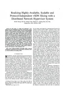
combination with the dynamicity of provisioning can enable a wide range of applications to run  significantly  more  efficiently,  due  to  efficient  task  dispatch  and  the  dynamic  resource  provisioning that simplify the compute resource management at the applications.   Micro‐benchmarks  show  that  Falkon  can  achieve  throughput  up  to  487  tasks/second  in  a  general case where each task is handled separately (with throughputs exceeding 2500 tasks/sec  with techniques similar to the clustering defined earlier), manage up to 54,000 executors, and  scale to 1.5 million queued tasks.   We conducted similar benchmarks on Condor and PBS to gain insight into how Falkon performs  as compared with those systems. We set the number of resources to 32 nodes (64 processors)  and  measured  the  time  to  complete  64  jobs  of  various  task  lengths  (ranging  from  1  sec  to  16384 sec). We then calculated the efficiency of resource usage as:  E = Sp / SI  Sp  is  the  practical  measured  speedup,  where  SI  is  the  ideal  speedup,  which  equals  to  the  number of processors being used. The maximum efficiency thus is 100%.   

Efficiency (64 processors)

1 0.9 0.8 0.7 0.6 0.5 0.4

Ideal Falkon Condor (v6.7.2) Condor (v6.9.3) PBS (v2.1.8)

0.3 0.2 0.1 0 1

10

100 1000 Task Length (sec)

10000

100000

  Figure 6: Efficiency of resource usage for varying task lengths on 64 processors comparing  Falkon, Condor and PBS   shows Falkon’s efficiency to be 95% with 1 sec tasks and 99% with 8 sec tasks. In contrast, both  PBS (v2.1.8) and Condor (v6.7.2) have an efficiency of less than 1% for 1 sec tasks and require  about 1,200 sec tasks to get 90% efficiency and 3,600 sec tasks to get 95% efficiency. They can  only achieve 99% efficiency with 16,000 sec tasks.   As both the PBS and Condor versions being tested on the experiment clusters (ANL/UC Teragrid  site) are not the latest versions, we also derived the efficiency curve for Condor version 6.9.3,  the latest development Condor version, which is claimed to have a throughput of 11 jobs/sec  [39] (up from our measured 0.5 jobs/sec and the 2 jobs/sec reported by others [32]). Efficiency  is much improved, reaching 90%, 95%, and 99% for job lengths of 50, 100, and 1000 seconds  respectively. The results in  for Condor v6.9.3 are derived, not measured. We derived based on  the  achieved  throughput  cited  in  [39]  of  11  tasks/sec  for  sleep  0  tasks.  Essentially,  we  computed the per task overhead of 0.0909 seconds, which we could then add to the ideal time  of  each  respective  task  length  to  get  an  estimated  task  execution  time.  With  this  execution 

time, we could compute speedup, which we then used to compute efficiency. Our derivation of  efficiency is simplistic, but it allowed us to plot the likely efficiency of the latest development  Condor code against the older production Condor code, the PBS production code, and Falkon. It  should  be  noted  that    illustrates  the  efficiency  of  these  systems  for  a  relatively  small  set  of  resources  (only  64  processors),  and  that  the  efficiency  gap  will  likely  only  increase  as  the  number  of  resources  increases  (see  Figure  7).    Also,    shows  only  the  efficiency  for  a  small  number  of  jobs  (64),  which  makes  slower  throughput  scenarios  (PBS  and  Condor)  hard  to  achieve high efficiency due to the large time to dispatch the tasks to the CPUs.  We therefore  generalize the results from  with the results in Figure 7.   We emphasize the need for such high throughputs by measuring the theoretical (assuming 1M  tasks)  resource  efficiency  at  three  different  scales  (small  grid  sites  –  100  processors,  medium  size grid site – 1K processors, large Grid – 10K processors) for various throughputs (1, 10, 100,  500,  1K,  10K,  100K,  and  1M  tasks/sec).  It  is  worth  noting  that  current  production  LRMs  (i.e.  throughput of 1 task/sec) require relatively long tasks in order to maintain high efficiency. For  example,  even  in  a  small  Grid  site  with  100  processors,  tasks  need  to  be  100  seconds  in  duration just to get 90% efficiency; the task duration is increased to 900 seconds for a modest  1K  processors,  10K  seconds  (~2.8  hours)  for  10K  processors  just  to  maintain  90%  efficiency.  With throughputs in the range of 500 tasks/sec (which is obtainable with Falkon), the same 90%  efficiency can be reached with tasks of length 0.2 seconds, 1.9 seconds, and 20 seconds for the  same three cases.  It should be evident that the higher the throughput of tasks/sec that can be  dispatched  and  executed  over  a  set  of  resources,  the  higher  the  resource  efficiency  for  the  same workloads and the faster the applications turn‐around times will be.    Small Grid Site (100 processors)

Medium Size Grid Site (1K processors)

100%

90%

80%

80%

80%

70%

70%

70%

60%

60%

60%

40%

Efficiency

90%

50%

50% 40%

50% 40%

30%

30%

30%

20%

20%

20%

10%

10%

0% 0.001

0.01

0.1

1

10

100

1000

10000

100000

Task Length (sec) 1 task/sec (i.e. PBS, Condor 6.8) 10 tasks/sec (i.e. Condor 6.9.2) 100 tasks/sec 500 tasks/sec (i.e. Falkon) 1K tasks/sec 10K tasks/sec 100K tasks/sec 1M tasks/sec

Large Grid (10K processors)

100%

90%

Efficiency

Efficiency

100%

10%

0% 0.001

0.01

0.1

1

10

100

1000

10000

100000

Task Length (sec) 1 task/sec (i.e. PBS, Condor 6.8) 10 tasks/sec (i.e. Condor 6.9.2) 100 tasks/sec 500 tasks/sec (i.e. Falkon) 1K tasks/sec 10K tasks/sec 100K tasks/sec 1M tasks/sec

0% 0.001

0.01

0.1

1

10

100

1000

10000

100000

Task Length (sec) 1 task/sec (i.e. PBS, Condor 6.8) 10 tasks/sec (i.e. Condor 6.9.2) 100 tasks/sec 500 tasks/sec (i.e. Falkon) 1K tasks/sec 10K tasks/sec 100K tasks/sec 1M tasks/sec

  Figure 7: Resource Efficiency for various resource scales and workload characteristics  Finally, we wanted to investigate the effects of the task dispatch rates on the I/O throughput  that could be achieved with Falkon and with Condor or PBS to and from the shared file system  and  compare  that  with  the  ideal  I/O  throughput  without  any  provisioning,  task  dispatch,  and  scheduling  overhead.  The  experiments  involved  the  execution  of  tasks  on  64  nodes  which  consisted of tasks with input and/or output with varying sizes from 1B to 1GB.  The shared file  system in this case was GPFS and it was configured with 8 I/O servers to handle the traffic in  and out of the shared file system. The results are shown in Figure 8. It is interesting to note that  Falkon (primarily due to the high dispatch rates it can achieve) can achieve close to the ideal I/O  throughput for both read performance.  On the other hand, Condor and PBS both require large  (i.e.  1GB)  input  and/outputs  per  job  in  order  to  achieve  the  same  level  of  performance  that  Falkon can achieve with significantly smaller input and outputs per job (i.e. 1MB).   

For  real  applications,  we  show  in  the  System  Evaluation  Section  that  Falkon  can  reduce  application  execution  time  significantly  (up  to  90%),  as  compared  with  other  job  submission  mechanisms, such as GRAM plus PBS.    4000

Throughput (Mb/s)

3500 3000 2500 2000

Falkon (GPFS R) Falkon (GPFS R+W) Condor/PBS (GPFS R) Condor/PBS (GPFS R+W) Ideal (GPFS R) Ideal (GPFS R+W)

1500 1000 500 0

Data Size (MB)

  Figure 8: The effect of task dispatch rates and how it affect I/O throughput 

5. SYSTEM EVALUATION  We  evaluate  various  aspects  of  the  Swift  system  using  both  synthetic  workloads  and  real  scientific  applications,  and  we  report  the  experiment  results  in  the  following  sections.  Unless  otherwise  specified,  the  experiments  used  a  machine  at  the  computation  institute  at  the  University of Chicago as the Swift submit host, and we used two computation clusters, one is  the  IA64  clusters  at  the  ANL/UC  TeraGrid  site  with  62  nodes,  and  the  other  the  computation  Institute Teraport cluster with 120 nodes. Both clusters had 1 Gb/s Ethernet connections and  used  PBS  as  the  default  local  scheduler.  We  summarize  the  configurations  of  the  test  environment  in  Table  2.  The  ANL_TG  cluster  was  used  as  the  default  execution  site  to  which  jobs were submitted.  Table 2     Configurations of the Test Environment  Name 

Type 

UC_SUBMIT 

Submit Host 

Location  UChicago CI  Workstation 

#nodes  1  62 

ANL_TG 

Execution Site 

ANL/UC  Teragrid Cluster  98 

UC_TP 

Execution Site 

UChicago CI  Teraport Cluster 

120 

Configuration  Intel P4 2.4GHZ  1 GB Memory  Intel Itanium 2   Dual Proc. 1.3 GHZ  4 GB Memory  Intel Xeon   Dual Proc. 2.4 GHZ  4 GB Memory  AMD Opteron   Dual Proc. 2.2 GHZ  4 GB Memory 

5.1.

Scalability  

We  consider  first  the  size  of  the  parallel  computations  that  can  be  executed  correctly.  Since  Swift integrates Karajan, we measure the maximum number of tasks (or the maximum number  of nodes in a task graph) that can be processed and dispatched with certain amount of memory  in both systems. Figure 9 shows the scalability results. For the Karajan measurement, we used a  simple  script  that  creates  multiple  parallel  threads;  each  of  the  threads  merely  waits  for  a  certain amount of time (so all the threads can be created before any of them terminates). In  doing so, we make sure that there is no extra overhead associated with each thread other than  the information necessary for its creation.   For the Swift measurement, we used a synthesized workflow where we could set the number of  nodes in the workflow and also the data dependencies (edges) between graph nodes. We set  the Java virtual machine (in which the Swift scheduler runs) heap size to use certain amount of  memory,  and  we  kept  adding  nodes  in  the  workflow  until  the  system  ran  out  of  memory  in  processing the workflow to get the maximum number of nodes. The Karajan system is shown to  be highly scalable, with 32 MB memory, it can create more than 40,000 threads. Each thread  has a memory footprint of 800 bytes, which is the base line as each thread only contains the  minimal information. Our Swift in general has much higher memory footprint (3.2 KB for each  node,  the  size  could  vary  with  different  workflow  graphs  and  procedure  definitions,  as  both  data  dependencies  and  input,  output  parameters  need  to  be  kept  in  memory),  but  can  still  support up to 4,000 threads with 32 MB memory, and 160,000 nodes with 1 GB memory. The  reason  each  node  takes  more  space  is  because  we  use  futures  for  data  synchronization,  and  each  future  object  wraps  a  java  dataset  object.  Also  for  each  node,  we  need  to  store  its  associated  procedure  information,  such  as  input,  output  names,  types  and  values  etc.  Nevertheless, the lightweight Karajan thread leaves much space for further improvement of our  Swift system.   200000 180000 Number of Nodes

160000 140000 120000 100000 80000 60000

Swift Karajan

40000 20000 0 0

200

400

600

800

1000

1200

Memory (MB)

  Figure 9 Swift System Scalability 

5.2.

Pipelining  

Our  SwiftScript  language  design  allows  us  to  implement  pipelining  across  iterations  (which  is  similar to the map operator in functional programming languages) for improved performance.  In  Swift,  we  realize  pipelining  using  the  future  mechanism  we  adopt  for  evaluating  data  dependencies. Pipelining allows us to dispatch jobs more efficiently as they become ready.   We evaluate the effect of pipelining in our implementation and show the result In . On the top,  we show the execution time for the fMRI workflow defined in Figure 1 without pipelining, and  on  the  bottom,  the  execution  time  with  pipelining.  The  workflow  operated  on  a  120‐volume  input dataset and involved four stages of 120 computations each. We can observe that the run  without  pipelining  had  to  wait  for  all  computations  in  one  stage  to  finish  before  it  could  proceed to the next stage, thus the distinct start times for all four stages. While in the pipelined  run, the computations between different stages were overlapped. Consequently, the execution  time was reduced by 21% for the fMRI workflow with pipelining enabled. 

 

  Figure 10 The Pipelining Effect for the fMRI Workflow 

5.3.

Load Balancing 

Load balancing is achieved in Swift using heuristics based on site responsiveness (Each site has a  score associated with its load and the turn‐around rate for job submissions). We tested system  load  balancing  also  using  the  120‐volume  input  fMRI  workflow,  and  we  configured  Swift  to  submit from UC_SUBMIT to both the ANL_TG and UC_TP clusters. Since UC_TP was in the same  local area network as that of the submit host, and the processors on UC_TP were faster than  those on ANL_TG, jobs dispatched to the UC_TP cluster completed faster, thus we can observe  in Figure 11 that overall the system balanced the load across the two sites, ANL_TG got 218 jobs  (in solid blue) out of the total number of 480, and UC_TP got the other 262 jobs (in solid gray),  and relatively more jobs were scheduled on the UC_TP cluster.  

  Figure 11  Load Balancing Across Two Clusters  We also notice the total execution time was cut down by 50% as compared with the execution  time  on  a  single  cluster  (ANL_TG).  The  reason  was  because  Swift  dispatched  jobs  to  the  two  sites simultaneously, and the overall queue wait time was reduced significantly, as jobs were in  two separate queues at the two sites, where each local scheduler dealt with only the jobs in its  queue.  As illustrated in the former Section, Swift can achieve great speedup by submitting jobs to the  Falkon service via the Falkon provider that we developed. Figure 12 shows both the throughput  of Swift via the Falkon provider, and the throughput of the Falkon service (tasks were submitted  from a Falkon client directly without going through Swift). In the experiment, the Falkon service  was run on the ANL_TG site, and we submitted both from a separate node within that cluster  (ANL‐>ANL),  and  from  the  UC_SUBMIT  host  (UC‐>ANL),  and  we  measured  the  throughput, 

defined as the number of sleep(0) jobs completed per second. We ran two worker threads on  32 nodes (as each node has dual processors) to get the numbers for 64 nodes.   We  measured  a  throughput  of  120  tasks  per  second  when  submitting  jobs  from  the  Falkon  client to the Falkon service directly in the same cluster, and a slightly lower throughput if we  ran the Falkon client at the UC_SUBMIT host. When Swift was used to submit the same set of  jobs, it was able to achieve up to 56 jobs per second in the LAN setting, and up to 46 jobs per  second  from  the  UC_SUBMIT  host.  Swift  incurred  a  large  overhead,  but  mainly  because  the  scheduling in Swift involves creation of a sandbox environment for each job (so that it does not  interfere with other concurrent running jobs on that node), and also logging and tracking of the  job execution processing. For each sleep job, many extra steps such as site selection, execution  directory setup and cleanup, exit code checking, etc were performed. In comparison, when jobs  were  submitted  from  the  Falkon  client,  it  involved  only  submission  and  getting  back  the  exit  code. Nevertheless, comparing with a standard setting when we use GT2 GRAM and PBS cluster  scheduler  where  we  can  only  get up to 2  jobs  per  second, the  throughput of  Swift  combined  with Falkon is improved by a factor of 23.  These performance numbers with Falkon are with an  older version that did not have all the latest optimizations we currently have in Falkon now; we  expect these numbers to further increase with the latest Falkon code base that can achieve as  high as 487 tasks/sec.  140 120

Throughput

100 80 60 40

Swift + Falkon (ANL->ANL) Swift + Falkon (UC->ANL) Falkon (ANL->ANL) Falkon (UC->ANL)

20 0 0

10

20

30

40

50

60

70

Number of Workers

  Figure 12 Swift throughput with the Falkon provider  We  further  compare  the  performance  of  submitting  from  Swift  to  providers  such  as  PBS  and  Falkon using real application examples in the next Section. 

5.4.

Application Performance  

Swift can either submit jobs via GRAM to a conventional batch scheduler such as PBS, in which  case  resource  provisioning  and  job  execution  are  combined  together,  or  it  can  submit  to  the  Falkon  execution  service,  where  resource  provisioning  is  separated  from  job  execution.  We  evaluate  the  effect  of  such  separation  using  three  examples:  1)  fMRI  (medical  imaging),  2)  Montage (astronomy), and 3) MolDyn (chemistry, molecular dynamics simulations). We repeat  the  fMRI  and  Montage  experiments  five  times  and  the  error  bars  indicate  the  standard  deviations of the measurements. These applications all involve stages that have large number  of small parallel jobs, a pattern that is common in many other scientific applications [41]. While  we can push hundreds or even thousands of such small jobs via GRAM to a PBS queue, they will  take  up  most  of  the  available  computing  nodes  but  at  the  same  time  only  achieve  low  throughput  due  to  queuing  overhead.  We  show  that  while  clustering  (bundling  a  number  of  small jobs into one large job) can help improve the throughput of such small jobs by 2 to 4 fold,  the  Falkon  service  can  improve  performance  7  to  10  fold  for  the  fMRI  application,  in  other  words, achieving up to 90% reduction in execution time. For the Montage application, Falkon  can achieve comparable performance to MPI execution.  In the case of MolDyn, we achieved an  8  fold  improvement  in  the  application  performance  when  comparing  Falkon  with  GRAM/PBS  submission.  

5.4.1.

fMRI (Medical Imaging Domain)  

We  note that  for  each  volume, each  individual task  in  the  fMRI  workflow  required  just  a few  seconds on an ANL_TG cluster node, so it is quite inefficient to schedule each job over GRAM  and  PBS,  since  the  overhead  of  GRAM  job  submission  and  PBS  resource  allocation  is  large  compared with the short execution time.  In Figure 13 we show the execution time for different  input data sizes for the fMRI workflow.   6000 5000

GRAM GRAM/Clustering Falkon

4808 3683

Time (s)

4000 3000

2510

2000 1239 1000

992

866 456

546

327

120

1123 678

0 120

240

360

480

Input Data Size (Volumes)

  Figure 13 Execution Time for the fMRI Workflow 

We  submitted  from  UC_SUBMIT  to  ANL_TG  and  measured  the  turnaround  time  for  the  workflows. A 120‐volume input (each volume consists of an image file of around 200KB and a  header file of a few hundred bytes) involves 480 computations for the four stages, whereas the  480‐volume input has 1960 computation tasks. The GRAM+PBS submission had low throughput  although it could have potentially used all the available nodes on the site (62 nodes to be exact,  as  we  only  used  the  IA64  nodes).  We  can  however  bundle  small  jobs  together  using  the  clustering mechanism in Swift, and we show the execution time was reduced by up to 4 times  (jobs were bundled into roughly 8 groups, as the grouping of jobs was a dynamic process) with  GRAM  and  clustering,  as  the  overhead  was  amortized  by  the  bundled  jobs.  The  Falkon  execution service (with 8 worker nodes) however further cuts down the execution time by 40‐ 70%, as each job was dispatched efficiently to the workers. We carefully chose the bundle size  for  the  clustering  so  that  the  clustered  jobs  only  required  8  nodes  to  execute.  This  choice  allowed  us  to  compare  GRAM/Clustering  against  Falkon,  which  used  8  nodes,  fairly.  We  also  experimented with different bundle sizes for the 120‐volume run, but the overall variations for  groups  of  4,  6  and  10  were  not  significant  (within  10%  of  the  total  execution  time  for  the  8  groups, plus or minus). 

5.4.2.

Montage (Astronomy Domain)  

The Montage  workflow demonstrated  similar  job  execution  time pattern  as there  were  many  small jobs involved. We show in Figure 14 the comparison of the workflow execution time using  Swift with clustering over GRAM, Swift over Falkon, and MPI. The Montage application code we  used  for  clustering  and  Falkon  are  the  same.  The  code  for  the  MPI  runs  is  derived  from  the  same  set  of  source  code,  with  the  addition  of  data  partitioning  and  inter‐processor  communication,  so  when  multiple  processors  are  allocated,  each  would  process  part  of  the  input  datasets,  and  combine  the  outputs  if  necessary.  The  MPI  execution  was  well  balanced  across multiple processors, as the processing for each image was similar and the image sizes did  not vary much. All three approaches needed to go over PBS to request for computation nodes,  we  used  16  nodes  for  Falkon  and  MPI,  and  also  configured  the  clustering  for  GRAM  to  be  around 16 groups.  The workflow had twelve stages, and we only show the parallel stages and the total execution  time in the figure (the serial stages ran on a single node, and the difference of running them  across  the  three  approaches  was  small,  so  we  only  included  them  in  the  total  time  for  comparison purposes). The workflow produced a 3x3 square degree mosaic around galaxy M16,  where there were about 440 input images (2MB each), and 2,200 overlappings between them.  There were two mAdd stages because we divided the region into subsets, co‐added images in  each subset, and then co‐added the subsets together into a final mosaic. We can observe that  the Falkon execution service performed close to the MPI execution, which indicated that jobs  were dispatched efficiently to the 16 workers. The GRAM execution with clustering enabled still  did  not  perform  as  well  as  the  other  two,  mainly  due  to  PBS  queuing  overhead.  It  is  worth  noting that the last stage mAdd was parallelized in the MPI version, but not for the version for  GRAM or Falkon, and hence the big difference in execution time between Falkon and MPI, and  the source of the major difference in the entire run between MPI and Falkon. 

3500 GRAM/Clustering

3000

MPI Falkon

Time (s)

2500 2000 1500 1000 500

al to t

d m Ad

) m Ad d( su b

nd m Ba ck gr ou

Fi t iff / m D

m Pr oj

ec t

0

Components

  Figure 14 Execution Time for the Montage Workflow  Katz  et  al.  [17]  have  also  created  a  task‐graph  implementation  of  the  Montage  code,  using  Pegasus.  They  did  not  implement  quite  the  same  application  as  us:  for  example,  they  ran  mOverlap and mImgtbl on the portal rather than on compute nodes, and they omitted the final  mAdd phase. Thus direct comparison with Swift over Falkon is difficult. However, if we omit the  final mAdd phase from the comparison, Swift over Falkon is then about 5% faster than MPI, and  thus also faster than the Pegasus approach, as they claimed that MPI execution time was the  lower bound for them. The reasons that Swift over Falkon performs better are that MPI incurs  initialization  and  aggregation  processes,  which  involve  multi‐processor  communications,  for  each  of  the  parallel  stages,  where  Falkon  acquires  resource  at  one  time  and  then  the  communications  in  dispatching  tasks  from  the  Falkon  service  to  workers  have  been  kept  minimum  (only  2  message  exchanges  for  each  job  dispatch).  The  Pegasus  approach  used  Condor’s  glide‐in  mechanism,  where  Condor  is  still  a  heavy‐weight  scheduler  compared  with  Falkon. 

5.4.3.

MolDyn (Chemistry Domain) 

We  further  illustrate  the  execution  process  in  Falkon  using  a  molecular  dynamics  (MolDyn)  application.  The  goal  of  this  study  is  to  optimize  and  automate  the  computational  workflow  that can be used to generate the necessary parameters and other input files for calculating the  solvation  free  energy  of  ligands,  and  can  also  be  extended  to  protein‐ligand  binding  energy.  Solvation  free  energy  is  an  important  quantity  in  Computational  Chemistry  with  a  variety  of  applications, especially in drug discovery and design. The accurate prediction of solvation free  energies of small molecules in water is still a largely unsolved problem, which is mainly due to  the  complex  nature  of  the  water‐solute  interactions.  In  the  study,  a  library  of  244  neutral 

ligands  is  chosen  for  free  energy  perturbation  calculations.  This  library  contains  compounds  with various chemical functional groups. Also, the absolute free energies of solvation for these  compounds are known experimentally, and will serve as a tool to benchmark our calculations.  All the structures were obtained from the NIST Chemistry WebBook database.  The MolDyn workflow consists of the following 8 stages:   •

Stage 1: Annotate each of the molecules in the study with charges.  

•

Stage  2:  For  each  molecule,  the  ligand  structures  are  modified  using  Antechamber  to  generate  the  individual  parameter  and  topology  files  for  CHARMM  Program.  Antechamber automatically detects the atom type, bond type and bond order from the  three‐dimensional geometry of the molecule, and generates the residue topology file. 

•

Stage 3: The ligand structure is equilibrated using CHARMM program.  

•

Stage 4: Compute the solvation energy using three coupling (staging) parameters using  the PERT module of the program CHARMM.  

•

Stage 6 computes the free energy for each of the resulting input configurations of each  molecule in the study using weighted histogram analysis method (WHAM).  

•

Stages 7 and 8 extract the free energy value from prior stages and put the final data into  a tabular form.  

Stage 1 is done once for all molecules in the workflow, stages 2‐8 are done for each molecule.  The number of jobs in the workflow is about 1 + 84N where N is the number of molecules. The  computation for each molecule takes about 235.4 minutes on one ANL_TG node processor, and  22.7  min  given  up  to  32  ANL_TG  nodes  (64  processors);  this  resulted  in  a  speedup  of  10.4x,  significantly less than 64 (the number of processors used at most), mostly due to the structure  of the workflow which had several stages which were not parallelizable.   shows the graphical  representation  of  each task  for  the  1  molecule experiment.    Red  denotes  wait  queue  time  in  Falkon and green denotes execution time per task.   

Task ID

Time (sec) 0 5 10 15 20 25 30 35 40 45 50 55 60 65 70 75 80 85

waitQueueTime execTime resultsQueueTime

Figure 15: MolDyn 1 Molecule Workflow Task View 

 

We were using the dynamic resource provisioning capabilities of Falkon in this experiment, and  hence resources were only allocated on demand when they were needed.  Notice the first job  queue time is about 81 seconds, essentially the time it took from when Falkon requested one  node  and  when  it  was  allocated  and  ready  to  process  work.    Then,  after  the  first  three  jobs  completed  in  serial  fashion),  there  was  a  stage  with  68  independent  jobs,  which  in  turn  triggered Falkon to allocated 31 more nodes (dual processors each) to be able to process all 68  independent  jobs  in  parallel.    The  red  lines  for  these  68  jobs  shows  the  time  delay  that  the  allocation  request  took  to  traverse  GRAM4  and  PBS  until  the  workers  were  ready  to  process  jobs.  To  better understand  the  structure  of  the  MolDyn  workflow,  we  show the  graph  structure  of  the workflow in Figure 16.  Notice the large amount of parallelism that is obtainable at various  stages of the workflow.  

  Figure 16: MolDyn Workflow Graph   showed the execution of 1 molecule, which is composed of 85 jobs that consume 235.4 CPU  minutes.    Our  next  experiment  performed  a  244  molecule  run,  which  is  composed  of  20497  jobs that should take less than 957.3 CPU hours to complete; in practice, it takes even less as 

some job executions are shared between molecules.  Figure 17 shows the resource utilization in  relation to Falkon queue length as the experiment progressed.  We see that as resources were  acquired  (using the dynamic  resource provisioning,  starting  with  0  CPUs  and  ending  with 216  CPUs at the peak), the CPU utilization was near perfect (green means utilized, red mean idle)  with  the  exception  of  the  end  of  the  experiment  as  the  last  few  jobs  completed  (the  last  43  seconds).      shows  the  same  information  on  a  per  task  basis,  while  Figure  18  shows  the  information on a per executor basis.  The entire experiment with the exception of the last 43  seconds consumed 866.33 CPU hours and wasted 0.09 CPU hours (99.98971% efficiency); if we  include  the  last  43  seconds  as  the  experiment  was  winding  down,  the  workflow  consumed  867.1  CPU  hours  and  it  wasted  1.78  CPU  hours,  with  a  final  efficiency  of  99.7949013%.    The  experiment completed in 15091 seconds on a maximum of 216 processors, which results in a  speedup of 206.9; note the average number of processors for the entire experiment was 207.26  CPUs, so the speedup of 206.9 reflects the 99.79% computed efficiency.      0

1800

3600

5400

7200

9000

10800

12600

14400

0

225 20000 200 17500 175 15000

10000

100

7500

75 50

5000

num_all_workers num_busy_workers waitQ_length delivered_tasks

25

2500

0

0 0

1800

3600

5400

7200 Time (sec)

9000

10800

12600

14400

Task ID

12500

125

Tasks

Executors

150

1 1001 2001 3001 4001 5001 6001 7001 8001 9001 10001 11001 12001 13001 14001 15001 16001 17001 18001 19001 20001

1800

3600

5400

Time (sec) 7200 9000 waitQueueTime

10800

execTime

12600

14400

resultsQueueTime

 

Figure 17: 244 Molecule MolDyn application; left: summary view showing executor’s  utilization in relation to the Falkon wait queue length as experiment time progressed; right:   task view showing per task wait queue time and execution time as experiment time  progressed  It  is  worth  comparing  the  performance  we  obtained  for  MolDyn  using  Falkon  with  that  of  MolDyn  over  traditional  GRAM/PBS.    Due  to  reliability  issues  (with  GRAM  and  PBS)  when  submitting 20K jobs over the course of hours, we were not able to successfully run the same  244 molecule run over GRAM/PBS.  We therefore tried to do some smaller experiments, in the  hopes that  it  would  increase  the  probability  of doing  a  successful  run.   We  tried  several runs  with  50  molecules  (4201  of  jobs  for  the  50  molecule  run,  instead  of  20497  jobs  for  the  244  molecule run); the best execution times we were able to achieve for the 50 molecule runs with  GRAM/PBS (on the same testbed as we have used for Falkon, using up to 200 processors) took  25292 seconds.  So we achieved a speedup of only 25.3X compared to 206.9X speedup when  using Falkon on the same workflow and the same Grid site in a similar state.   

  Figure 18 244 Molecule MolDyn application: Executor’s view showing each task that it  executed (green) delineated by the black vertical bars showing each task boundary 

We explain this drastic difference mostly due to the typical job duration (~200 seconds) and the  submission rate throttling of 1/5 jobs per second; the best case scenario is that the workflow  could  have  kept  40  machines  busy,  but  in  reality  the  number  of  concurrent  jobs  ranged  between  30~40  jobs.  Increasing  the  submission  rate  throttle  resulted  in  GRAM/PBS  gateway  instability,  or  even  causing  it  to  stop  functioning.    Furthermore,  each  node  was  only  using  a  single  processor  of  the  dual  processors  available  on  the  compute  nodes  due  to  the  local  site  PBS policy that allocates each job an entire (dual processor) machine and does not allow other  jobs  to  run  on  allocated  machines;  it  is  left  up  to  the  application  to  fully  utilize  the  entire  machine, through multi‐threading, or by invoking several different jobs to run in parallel on the  same machine.  This is a great example of having a system like Falkon that allows the specific  configuration  of  new  queues  that  behave  appropriately  on  a  per  application  basis,  which  is  quite impractical to do (mostly due to policy) in real‐world deployed Grids. 

5.4.4.

Application Summary  

The evaluation of the Swift runtime system shows that it is fast and scalable in executing large  scale  scientific  computations.  Swift  leverages  lightweight  threading  techniques  and  can  schedule  hundreds  of  thousands  of  parallel  computations  efficiently;  its  combination  of  type  checking, retry mechanism and restart log supports reliable workflow execution. The abstract  provider  interface  and  various  implementations  allow  workflows  to  be  executed  either  on  a  single  desktop,  on  a  cluster  managed  by  a  batch  scheduler,  or  on  multi‐site  distributed  resources. The integration with the lightweight Falkon execution service significantly improves  system throughput for large number of small jobs. In particular, we show that Swift plus Falkon  can achieve comparable performance to MPI execution for the Montage workflow, and also can  reduce  execution  time  by  as  much  as  90%  for  the  fMRI  pipeline  when  compared  with  GRAM  and PBS submission.  We also showed a large scale MolDyn workflow with 20K tasks that was  able to achieve 99.8% efficiency on 216 processors over a period of 15K seconds; Falkon was  able to achieve an application speedup of 206.9X when GRAM/PBS was only able to achieve a  25.3X speedup on the same Grid site with similar usage conditions.    

6. CONCLUSION 

 

We have discussed the motivations for providing a high level abstraction of data, programs and  computations in large scale Data Grid environments, and challenges inherent in attempting to  do  so,  and  we  have  proposed  a  scripting  language  for  concise  specifications  of  large  scale  parallel  computations  on  file  system  data  and  a  runtime  system  to  support  data,  workflow,  metadata, and provenance management. We have shown that the Swift language and system  support efficient description, compilation, execution and optimization of parallel computations,  using  examples  from  large‐scale  scientific  experiments  in  domains  such  as  astronomy,  biochemistry, and neuroscience.  SwiftScript  is  a  parallel  program  notation  that  cleanly  separates  logical  data  structures  from  their physical storage formats, by means of the underlying XDTM mechanism. XDTM employs a  two‐level description of datasets, defining separately via a type system based on XML Schema  the abstract structure of datasets, and the mapping of that abstract data structure to physical  representations.  The  dataset  mapping  mechanism  allows  physical  datasets  to  be  mapped  to 

logical data structures, thus enabling SwiftScript to represent dynamic workflow structures and  expand workflow nodes during run time. SwiftScript models file system data as first‐class typed  objects, and allows for the definitions of concise typed procedures that operate on these typed  datasets,  and  the  composition  of  complex  scientific  workflows  from  simple  and  compound  procedures.  Its  support  for  dataset  selection  and  iteration  enables  a  SwiftScript  program  to  scale  easily  to  tens  of  thousands  of  computations.  Programs  written  in  SwiftScript  are  much  more compact in code size, and also easier to read, understand and maintain.  The  runtime  system  Swift  provides  the  automated  mechanism  to  compile  logical  workflow  representations  into  concrete  distributed  execution  plan,  manage  and  coordinate  distributed  computing, network and storage resource for the efficient and reliable execution of the plan,  monitor  and  record  the  execution  process,  and  trace  the  derivation  history  of  data  products.  The  provenance  of  data  derivations  is  captured  and  stored  in  VDC  along  with  dataset,  procedure and workflow definitions; together they allow powerful exploration and expressive  query of the virtual data products.  Swift  integrates  and  extends  the  CoG  Karajan  engine,  whose  abstract  provider  interface  supports submission to different computing facilities ranging from local desktops, to computer  clusters  and  multi‐site  Grid  environments.  By  leveraging  the  lightweight  Falkon  execution  service, Swift is able to achieve high throughput in executing large number of fine‐granular jobs,  a  common  pattern  we  find  in  both  the  fMRI  and  Montage  workflows,  and  other  scientific  applications.   In conclusion, the language and system together can bring significant usability and productivity  increases,  in  representing  and  executing  large  scale  scientific  workflows,  and  in  facilitating  discovery,  understanding,  assessment,  and  sharing  of  data,  procedures,  workflows  and  computation  resources,  as  well  as  in  the  productive  use  of  distributed  resources  for  computation, scheduling, and collaboration.  For  future  directions,  we  continue  to  work  to  improve  the  language  and  system  to  deal  with  other requirements and characteristics in large scale scientific computations. In particular, we  are working on more intuitive invocation interface (the specification of how an application or  service  is  invoked)  in  SwiftScript  and  easier  mapper  implementation.  SwiftScript  mappers  are  currently  specified  as  Java  classes.  Pre‐coded  mappers  work  well  for  applications  with  structured  file  collections  such  as  in  the  fMRI  and  Montage  cases,  but  other  customized  mappers  are  required  for  more  complex  data  structures,  and  the  implementation  of  such  mappers are not trivial.  Data  partitioning  is  an  important  issue  in  harnessing  parallel  and  distribute  computing  resources.  Iterations  in  SwiftScript  allow  programs  to  operate  on  the  finest  level  of  datasets.  However, SwiftScript currently does not support coarse level data partitioning, such as blocked  or  cyclic  partition  that  are  commonly  observed  in  data  parallel  programs.  We  consider  extending  SwiftScript  with  (optional)  data  partitioning  directives,  and  give  experienced  user  more control over the data being processed.  We are also investigating data locality aware scheduling strategies. [43] Most cluster execution  environments have a shared file system, where input and output datasets are staged in to and 

out  from.  This  shared  medium  becomes  a  bottleneck  when  a  large  number  of  I/O  intensive  computations  are  executed  in  the  cluster,  although  the  computing  resource  may  not  have  saturated. Considering that each node in a cluster usually has its own local disks, and local disk  access is at least as fast, if not faster than a shared storage space, we can cache and replicate  intermediate  computation  results  on  local  disks,  and  make  scheduling  decisions  according  to  the availability of the intermediate data, i.e. choosing the compute node that has most of the  required  data  for  a  job.  Such  a  strategy  could  further  increase  the  number  of  parallel  computations and improve system throughput.  Currently  most  of  the  applications  we  deal  with  are  binary  executables  that  operate  on  file  system  based  data.  However,  our  SwiftScript  programming  model  can  be  equally  applied  to  Web  services  invocation  and  coordination.  SwiftScript  specifies  abstract  interfaces  to  procedures, which can be bound to service invocations at runtime, and the XDTM data model is  based  on  XML  Schema,  which  can  naturally  capture  Web  service  inputs  and  outputs.  While  Service Oriented Architecture is gaining adoption, SwiftScript can provide a bridge between the  application and service deployment models. 

7. ACKNOWLEDGEMENT  We would like to thank Bruce Berriman, Daniel Katz, and John Good for their help and support  on  the  Montage  application.  Montage  is  supported  by  the  NASA  Earth  Sciences  Technology  Office Computing Technologies program, under Cooperative Agreement Notice NCC 5‐6261.   We would also like to thank Ben Clifford, Gregor Von Laszewski, and Tiberiu Stef‐Praun for their  contributions  to  the  Swift  system.  The  evaluation  of  the  Swift  system  was  carried  out  on  computing  facilities  at  the  Computation  Institute  at  the  University  of  Chicago,  and  at  the  Teragrid ANL/UC site.   This work was supported by the National Science Foundation GriPhyN Project, grant ITR‐800864  and  iVDGL,  grant  PHY‐122557;  I2U2  –  Interactions  in  Understanding  the  Universe,  grant  PHY‐ 0636265; the Mathematical, Information, and Computational Sciences Division subprogram of  the  Office  of  Advanced  Scientific  Computing  Research,  U.S.  Department  of  Energy  under  contract DE‐AC02‐06CH11357; the National Institutes of Health, grants NS37470, NS44393 and  DC008638‐01; and NASA Ames Research Center GSRP Grant Number NNA06CB89H. 

8. REFERENCES  [1]

Andrews, T., Curbera, F., Dholakia, H., Goland, Y., Klein, J., Leymann, F., Liu, K., Roller, D.,  Smith, D., Thatte, S., Trickovic, I., Weerawarana, S.: Business Process Execution Language  for Web Services, Version 1.1. Specification, BEA Systems, IBM Corp., Microsoft Corp., SAP  AG, Siebel Systems (2003).  

[2]

Arbree,  A.,  Avery,  P.,  Bourilkov,  D.,  Cavanaugh,  R.,  Graham,  G.,  Rodriguez,  J.,  Wilde, M.,  Zhao, Y.: Virtual Data in CMS Analysis. Proceedings of the 2003 Conference for Computing  in High‐energy and Nuclear Physics (CHEP 03). 

[3]

Armstrong, J., Virding, R., Wikström, C., Williams, M., Concurrent Programming in Erlang,  Prentice‐Hall, 1996, ISBN 0‐13‐285792‐8, 2nd edition. 

[4]

Business Process Modeling Language 1.0 Specification, http://www.bpmi.org/, 2002 

[5]

Churches,  D.,  Gombas,  G.,  Harrison,  A.,  Maassen,  J.,  Robinson,  C.,  Shields,  M.,  Taylor,  I.,  Wang,  I.,  Programming  Scientific  and  Distributed  Workflow  with  Triana  Services.  Concurrency  and  Computation:  Practice  and  Experience.  Special  Issue  on  Scientific  Workflows, 2005. 

[6]

The  Condor  DAGMan  (Directed  http://www.cs.wisc.edu/condor/dagman, 2007. 

[7]

Cytron, R. Ferrante, J., Rosen, B., Wegman, M., and Zadeck, F., Efficiently computing static  single  assignment  form  and  the  control  dependence  graph.  ACM  Transactions  on  Programming Languages and Systems, 13(4):451‐490, Oct 1991. 

[8]

Dean,  J.  and  Ghemawat,  S.,  MapReduce:  Simplified  data  processing  on  large  clusters.  In  OSDI, 2004. 

[9]

Deelman,  E.,  Singh,  G.,  Su,  M.‐H.,  Blythe,  J.,  Gil,  Y.,  Kesselman,  C.,  Mehta,  G.,  Vahi,  K.,  Berriman,  G.B.,  Good,  J.,  Laity,  A.,  Jacob,  J.C.  and  Katz,  D.S.  Pegasus:  A  Framework  for  Mapping Complex Scientific Workflows onto Distributed Systems. Scientific Programming,  13 (3). 219‐237. 

Acyclic 

Graph 

Manager), 

[10] Emmerich,  W.,  Butchart,  B.,  Chen,  L.,  Wassermann,  B.  and  Price,  S.  Grid  Service  Orchestration  Using  the  Business  Process  Execution  Language  (BPEL).  Journal  of  Grid  Computing, 3 (3‐4). 283‐304.  [11] Foster,  I.,  Globus  Toolkit  Version  4:  Software  for  Service‐Oriented  Systems.  IFIP  International Conference on Network and Parallel Computing, 2005, Springer‐Verlag LNCS  3779, 2‐13.  [12] Foster,  I.,  Voeckler,  J.,  Wilde,  M.  and  Zhao,  Y.  Chimera:  A  Virtual  Data  System  for  Representing, Querying, and Automating Data Derivation. in 14th Conference on Scientific  and Statistical Database Management, (2002).  [13] Halsted.  R.  H.,  Multilisp:  A  language  for  concurrent  symbolic  computation.  ACM  Transactions on Programming Languages and Systems 7(4), pages 501‐‐538, April 1985.  [14] High  Performance  Fortran  Forum.  High  Performance  Fortran  Language  Specification.  Technical report, Rice University, Dept. Computer Science, October 1992.  [15] Horn, J.V., Dobson, J., Woodward, J., Wilde, M., Zhao, Y., Voeckler, J. and Foster, I. Grid‐ Based Computing and the Future of Neuroscience Computation. in Methods in Mind, MIT  Press, 2006.  [16] Huettel,  S.,  Song,  A.  and  McCarthy,  G.  Functional  Magnetic  Resonance  Imaging.  Sinauer  Associates, 2004.  [17] Katz, D., Berriman, G., Deelman, E., Good, J., Jacob, J., Kesselman, C., Laity, A., Prince, T.,  Singh,  G.,  and  Su,  M.  A  Comparison  of  Two  Methods  for  Building  Astronomical  Image  Mosaics on a Grid, Proceedings of the 7th Workshop on High Performance Scientific and  Engineering Computing (HPSEC‐05), 2005 

[18] Laszewski,  G.v.,  Hategan,  M.  and  Kodeboyina,  D.  Java  CoG  Kit  Workflow,  in  Taylor,  I.J.,  Deelman, E., Gannon, D.B. and Shields, M. eds. Workflows for eScience, 2007, 340‐356.  [19] Ludäscher, B., Altintas, I., Berkley, C., Higgins, D., Jaeger‐Frank, E., Jones, M., Lee, E., Tao,  J.,  Zhao,  Y.,  Scientific  Workflow  Management  and  the  Kepler  System.  Concurrency  and  Computation: Practice & Experience, Special Issue on Scientific Workflows, 2005.  [20] Mohr,  E.,  Kranz,  D.A.,  Halsted,  R.  H.:  Lazy  Task  Creation:  A  Technique  for  Increasing  the  Granularity  of  Parallel  Programs,  Proceedings  of  the  ACM  Conference  on  Lisp  and  Functional Programming. 1990.  [21] The Montage project web page, http://montage.ipac.caltech.edu/, 2007  [22] Moreau  L,  Zhao  Y,  Foster  I,  Voeckler  J,  and  M  Wilde.  XDTM:  XML  Dataset  Typing  and  Mapping for Specifying Datasets. In European Grid Conference, 2005.  [23] M. P. I. Forum. MPI: A Message‐Passing Interface Standard, May 1994.  [24] Mueller, F., A library implementation of POSIX threads under UNIX, 1993 winter USENIX,  San Diengo, CA, January 25‐29, 1993.  [25] Oinn, T., Addis, M., Ferris, J., Marvin, D., Senger, M., Greenwood, M., Carver, T., Glover, K.,  Pocock,  M.  R.,  Wipat,  A.,  Li,  P.,  Taverna:  A  tool  for  the  composition  and  enactment  of  bioinformatics workflows. Bioinformatics Journal, 20(17):3045–3054, 2004.  [26] OpenMP:  a  Proposed  Industry  Standard  API  for  Shared  Memory  Programming.  White  Paper, http://www.openmp.org/, October 1997.  [27] Pike,  R.,  Dorward,  S.,  Griesemer,  R.,  Quinlan,  S.,  Interpreting  the  Data:  Parallel  Analysis  with  Sawzall,  Scientific  Programming,  Special  Issue  on  Grids  and  Worldwide  Computing  Programming Models and Infrastructure 13:4, pp. 227‐298.  [28] The Provenance Challenge, http://twiki.ipaw.info/bin/view/Challenge/WebHome, 2006.  [29] Raicu,  I.,  Dumitrescu,  C.  and  Foster,  I.,  “Dynamic  Resource  Provisioning  in  Grid  Environments”, TeraGrid Conference 2007, June 2007.  [30] Raicu,  I.,  Zhao,  Y.,  Dumitrescu,  C.,  Foster,  I.,  Wilde,  M.,  “Falkon:  a  Fast  and  Lightweight  Task Execution Framework”, IEEE/ACM Supercomputing (SC’07), November 2007.  [31] Reppy,  J.  H.  Concurrent  Programming  in  ML.  Cambridge  University  Press,  Cambridge,  England, 1999.  [32] Robinson,  E.,  DeWitt,  D.  J.,  “Turning  Cluster  Management  into  Data  Management:  A  System Overview”, Conference on Innovative Data Systems Research, 2007.  [33] Sloan Digital Sky Survey Data Release 6, http://www.sdss.org/dr6  [34] The TeraGrid, http://www.teragrid.org, 2007.  [35] Thain,  D.,  Tannenbaum,  T.,  Livny,  M.,  Distributed  Computing  in  Practice:  The  Condor  Experience, Concurrency and Computation: Practice and Experience, 2004. 

[36] Vöckler,  J.‐S.,  Mehta,  G.,  Zhao,  Y.,  Deelman,  E.  and  Wilde,  M.,  Kickstarting  Remote  Applications. in 2nd International Workshop on Grid Computing Environments (2006).   [37] Welsh,  M.,  Culler,  D.,  and  Brewer,  E.,  SEDA:  An  Architecture  for  Well‐Conditioned,  Scalable  Internet  Services.  In  Proceedings  of  the  Eighteenth  Symposium  on  Operating  Systems Principles (SOSP‐18), Banff, Canada, October, 2001.   [38] XML  Process  Definition  Language  (XPDL)  (WFMCTC‐1025).  Technical  report,  Workflow  Management Coalition, Lighthouse Point, Florida, USA, 2002.   [39] T. Tannenbaum. “Condor RoadMap”, Condor Week 2007.  [40] Zhao, Y., Dobson, J., Foster, I., Moreau, L. and Wilde, M. A Notation and System for  Expressing and Executing Cleanly Typed Workflows on Messy Scientific Data. SIGMOD  Record, 34 (3). 37‐43. 2005.  [41] Zhao, Y., Hategan, M., Clifford, B., Foster, I., Laszewski, G.v., Raicu, I., Stef‐Praun, T., Wilde,  M., Swift: Fast, Reliable, Loosely Coupled Parallel Computation, IEEE International  Workshop on Scientific Workflow (SWF07), Collocated with ICWS 2007.  [42] Zhao, Y., Wilde, M., Foster, I., Applying the Virtual Data Provenance Model, Proceedings of  the International Provenance and Annotation Workshop 2006 (IPAW2006), Lecture Notes  in Computer Science, Springer, 2006.  [43] I. Raicu, I., Zhao, Y., Foster, I., Szalay, A. “A Data Diffusion Approach to Large Scale  Scientific Exploration,” Microsoft eScience Workshop at RENCI 2007.