Recent Developments in Context-Based Predictive Techniques for Lossless Image Compression N ASIR M EMON 1
AND
X IAOLIN W U 2
1
2
Department of Computer Science, Northern Illinois University, DeKalb, IL, 60115, USA Department of Computer Science, The University of Western Ontario, London, Ontario, Canada N6A 5B7 Email:
[email protected]
In this paper we describe some recent developments that have taken place in context-based predictive coding, in response to the JPEG/JBIG committee’s recent call for proposals for a new international standard on lossless compression of continuous-tone images. We describe the different prediction techniques that were proposed and give a performance comparison. We describe the notion of context-based bias cancellation, which represents one of the key ideas that was proposed and incorporated in the final standard. We also describe the different error modelling and entropy coding techniques that were proposed for encoding prediction errors, the most important development here being an ingeniously simple and effective technique for adaptive Golomb–Rice coding. We conclude with a short discussion on avenues for future research. Received July, 1996; revised May, 1997
1. INTRODUCTION We have seen an increased level of activity in image and video compression in recent years; however, most of this activity has been restricted to lossy compression. Many applications, such as medical imaging, image archiving, high-precision image analysis, remote sensing, pre-press imaging, preservation of art work and historical documents, require lossless compression. Despite the importance of lossless image compression of continuous-tone images there is a paucity of standard algorithms. Current standards for lossless compression include 1. 2. 3.
Lossless JPEG (Huffman and arithmetic). JBIG, Group 4 Fax. GIF, Photo CD, PNG etc.
It is generally accepted that the Huffman-coding-based JPEG lossless standard provides poor compression and a host of better techniques have been reported in the literature [1– 3]. The JPEG arithmetic coding version does provide about 10% better compression, but is not available in the public domain and hence has seen little use. JBIG and the CCITT Group 3 and 4 standards are primarily designed for bi-level data and do not provide good compression when used on greyscale images by compressing individual bit planes. GIF and PNG are essentially suitable for synthesized images and are known not to work well with natural continuous-tone images acquired through an array of sensors. Due to the perceived inadequacy of current standards for lossless image compression, the JBIG/JPEG committee of
the International Standards Organization (ISO) approved a new work item proposal in early 1994, titled Next Generation Lossless Compression of Continuous-tone Still Pictures. A call was issued in March 1994 soliciting proposals specifying algorithms for lossless and near-lossless compression of continuous-tone (2–16 bit) still pictures. A number of requirements were imposed on submissions; for details the reader is referred to [4]. For instance, exploitation of interband correlations (in colour and satellite images for example) was prohibited. This call for proposals resulted in renewed activity focused on the development of lossless image compression techniques. A large part of this activity has focused on a specific type of compression technique, loosely referred to in the literature as lossless DPCM or lossless predictive coding. Since the baseline algorithm that has been standardized [5] and the proposed high-performance extension both employ a predictive coding approach, we restrict our discussion to predictive coding techniques. We describe some of the important new developments that emerged in response to the call for proposals, and have contributed significantly to the advancement in the state of the art of predictive coding techniques for lossless image compression. The paper is structured as follows. In the next section we begin by giving an introduction to predictive coding techniques for lossless image compression and describe the current lossless JPEG standard. We also introduce and establish some terminology and notation that is used throughout the rest of the paper. In Section 3 we describe various predictors that were proposed. We describe three specific predictors,
T HE C OMPUTER J OURNAL, Vol. 40,
No. 2/3,
1997
128
N. M EMON AND X. W U
i
NW WW
W
NN
NNE
N
NE
TABLE 1. JPEG predictors for lossless coding Mode 0 1 2 3 4 5 6 7
P[i, j]
j
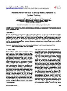
FIGURE 1. Notation used for specifying neighbouring pixels of the current pixel P[i, j].
MED, GAP and ALCM in detail and then present a performance comparison which clearly establishes the choice of MED as the default predictor for the standard. In fact, an important discovery made during the standardization process was the surprising efficacy of the MED predictor despite its apparent simplicity. In Section 4 we describe the notion of context-based bias cancellation, which was one of the key ideas that contributed towards the development of the final standard. In Section 5 we outline the different error modelling techniques that were proposed for encoding prediction errors and in Section 6 we describe the specific entropy coding techniques employed. The most important contribution here came from the revised LOCO algorithm proposed by HP laboratories [6, 7], in the form of a very simple and effective parameter estimation technique for Golomb–Rice coding. We conclude in Section 7 with a discussion on avenues for further research in lossless image compression. At this point we would like to note that it is not the intention of this paper to give a detailed description of the new lossless JPEG standard, nor do we intend this to be a thorough treatise on lossless image compression in general. Our intention is to describe the main ideas that were proposed in response to the JPEG committee’s call for proposals, the convergence of which led to the development of the new standard. 2. PREDICTIVE CODING TECHNIQUES AND THE CURRENT JPEG LOSSLESS STANDARD Among various methods which have been devised for lossless compression, predictive techniques are perhaps the simplest and most efficient. Here the transmitter (and receiver) process the image in some fixed order (say, raster order going row by row, left to right within a row) and predict the value of the current pixel on the basis of the pixels which have already been transmitted (received). If we denote the current ˆ j], then only pixel by P[i, j] and its predicted value by P[i, ˆ j] − P[i, j], needs to be the prediction error, e = P[i, transmitted. If the prediction is reasonably accurate then the distribution of prediction errors is concentrated near zero and has a significantly lower zero-order entropy than the original image. If the residual image consisting of prediction errors is treated as an Independent and Identically Distributed (IID) source, then it can be coded efficiently using any of the
Prediction for P[i, j] 0 (no prediction) N W NW N + W − NW W + (N − NW)/2 N + (W − NW/2 (N + W )/2
standard variable-length entropy coding techniques, such as Huffman coding or arithmetic coding. Unfortunately, even after applying the most sophisticated prediction techniques, generally the residual image has ample structure which violates the IID assumption. Hence, in order to encode prediction errors efficiently we need a model that captures the structure that remains after prediction. This step is often referred to as error modelling [8]. The error modelling techniques employed by most lossless compression schemes proposed in the literature can be captured within the context modelling framework described in [9] and applied in [9, 10]. In this approach, the prediction error at each pixel is encoded with respect to a conditioning state or context, which is arrived at from the values of previously encoded neighbouring pixels. Viewed in this framework, the role of the error model is essentially to provide estimates of the conditional probability of the prediction error, given the context in which it occurs. This can be done by estimating the PDF by maintaining counts of symbol occurrences within each context [10] or by estimating the parameters (variance, for example) of an assumed Probability Density Function (PDF) (Laplacian, for example) as in [8]. In Figure 1 we show a template of two-dimensional neighbourhood pixels, a subset of which is generally used for prediction and/or context determination by lossless image compression techniques. In the remainder of the paper we use the notation specified in Figure 1 to denote specific neighbours of the pixel P[i, j] in the ith row and jth column. 2.1.
The current lossless JPEG standard
The current JPEG standard uses a predictive scheme when used in its lossless mode. It provides eight different predictors from which the user can select. Table 1 lists the eight predictors used. The prediction errors are then encoded either by Huffman coding or arithmetic coding—codecs for both are provided by the standard. In the Huffman coding version, essentially no error model is used. The prediction errors are assumed to be IID and either a static default Huffman table is used or a custom Huffman code table can be specified, which is then encoded along with the compressed image. The latter approach requires two passes through the data. The arithmetically coded version uses quantized prediction errors at neighbouring pixels as contexts for
T HE C OMPUTER J OURNAL, Vol. 40,
No. 2/3,
1997
L OSSLESS I MAGE C OMPRESSION conditioning the prediction error. Binary arithmetic coding is used within each context by decomposing the prediction error into a sequence of binary decisions. The first binary decision determines whether the prediction error is zero. If it is not zero, then the second step determines the sign of the error. The subsequent steps assist in classifying the magnitude of the prediction error into one of a set of ranges and the final bits that determine the exact prediction error magnitude within the range are sent uncoded. The QM-Coder is used for encoding each binary decision. A detailed description of the coder and the standard can be found in [11]. Given the success of predictive techniques for lossless image compression, it was no surprise that seven out of the nine proposals submitted to ISO, in response to the call for proposals for a new lossless image compression standard, employed prediction followed by conditional encoding of the prediction error. In this paper we restrict our discussion to these seven proposals. The other two proposals [12, 13] were based on transform coding. However, right from the first-round evaluations it was clear that the transform-codingbased proposals did not provide as good compression ratios as algorithms proposed based on predictive techniques [14]. In the remainder of this paper we describe in more detail the specific contributions that were made which have led to the development of the new proposed standard.
candidate predictors. Martucci reported the best results with the following three predictors, in which case it is easy to see that MAP turns out to be the MED predictor. 1. 2. 3.
3.2.
The GAP predictor
The CALIC proposal [17] included a gradient-adjusted predictor (GAP) which adapts the prediction according to local gradients and hence gives a more robust performance compared to standard linear predictors. GAP weights the neighbouring pixels of P[i, j] according to the estimated gradients in the neighbourhood. In GAP the gradient of the intensity function at the current pixel P[i, j] is estimated by computing the following quantities: dh = |W − WW| + |N − NW| + |N − NE| dv = |W − NW| + |N − NN| + |NE − NNE|.
(1)
ˆ j] is then made by the following proceA prediction P[i, dure: IF (dv − dh > 80) {sharp horizontal edge} ˆ j] = W P[i, ELSE IF (dv − dh < −80) {sharp vertical edge} ˆ j] = N P[i, ELSE { ˆ j] = (N + W )/2 + (NE − NW)/4; P[i, IF (dv − dh > 32) {horizontal edge} ˆ j] = ( P[i, ˆ j] + W )/2 P[i, ELSE IF (dv − dh > 8) {weak horizontal edge} ˆ j] = (3 P[i, ˆ j] + W )/4 P[i, ELSE IF (dv − dh < −32) {vertical edge} ˆ j] = ( P[i, ˆ j] + N )/2 P[i, ELSE IF (dv − dh < −8) {weak vertical edge} ˆ j] = (3 P[i, ˆ j] + N )/4 P[i, }
In this section we briefly describe the predictors that were proposed. At the end of the section we give a performance comparison and make a few observations. 3.1. The MED predictor
The MED predictor has also been called MAP (median adaptive predictor) and was first proposed by Martucci [15]. Martucci presented the MAP predictor as a non-linear adaptive predictor that selects the median of a set of three predictions in order to predict the current pixel. One way of interpreting such a predictor is that it always chooses either the best or the second-best predictor among the three
N W N + W − NW.
In an extensive evaluation, the MED predictor was observed to give superior performance over most linear predictors [16].
3. THE PREDICTION STEP
Hewlett Packard’s proposal, LOCO-I (low-complexity lossless coder) [6], used the median edge detection (MED) predictor, that adapts in the presence of local edges. MED detects horizontal or vertical edges by examining the North (N ), West (W ) and North-West (NW) neighbours of the current pixel P[i, j] as illustrated in Figure 1 in Section 2. The North pixel is used as a prediction in the case of a vertical edge being detected. The West pixel is used as a prediction in the case of a horizontal edge. Finally, if neither a vertical edge nor a horizontal edge is detected, planar interpolation is used to compute the prediction value. Specifically, prediction is performed according to the following equations: if NW ≥ max(N , W ) min(N , W ) ˆ j] = max(N , W ) if NW ≤ min(N , W ) P[i, N + W − NW otherwise.
129
where N, W, NW, NN, NE and NNE are as defined in Figure 1. The thresholds given in the above procedure are for 8bit data and are adapted on the fly for higher resolution images. These thresholds were arrived at after extensive experimentation with a large set of test images. 3.3.
The ALCM and JSLUG predictor
The ALCM proposal [18] and the JSLUG proposal [19] included an adaptive predictor that used a weighted combination of five neighbourhood pixels in order to predict the current pixel. The weights are adapted on the fly as encoding progresses. The neighbourhood used consisted of the N, W, NW, NE and WW pixels as specified in Figure 1.
T HE C OMPUTER J OURNAL, Vol. 40,
No. 2/3,
1997
130
N. M EMON AND X. W U
Initially, all pixels are assigned an equal weight. After prediction, the weights are changed as follows. If the prediction was lower than the actual value then the weight 1 and of the largest neighbouring pixel is decremented by 256 the weight of the smallest neighbour is decremented by the same amount. If the prediction was too high then the largest neighbouring pixel is decremented and the smallest one is incremented. In case more than one pixel has the highest weight, ties are broken by using the following priority scheme. 1 5
4
2
TABLE 2. Zero-order entropy of prediction errors with the MED, GAP and ALCM predictors
3
P[i, j]
The pixel labelled 1 is changed with highest priority and the pixel labelled 5 with least priority. 3.4. Other predictors Besides MED, GAP and ALCM, there were a few more predictors proposed in different submissions, but a detailed evaluation revealed their performance to be inferior [20]. For example, the Mitsubishi proposal, CLARA [21], adaptively switched between a fixed set of predictors based on the texture and gradients in the neighbourhood of the target pixel. The following set of predictors was used: N,
W,
N +W , 2
N N + NE + . 2 4
Details of the exact manner in which the selection was made are given in [21]. Another predictor, given in the DARC proposal by Kodak [22], adapted to horizontal and vertical gradients in the neighbourhood of the pixel being predicted. Specifically, ˆ i, ˆ j] = αW + given that the current pixel is predicted to be P[ (1 − α)N where 1v 1h + 1v 1v = |W − NW| α=
1h = |N − NW|.
Image
ALCM
MED
GAP
Air1 Air2 Bike Bike3 Cafe Cats Chart Chart s Compound1 Compound2 CR CT Faxballs Finger Gold Graphic Hotel MRI Tools Ultra-Sound Water Woman X-ray
8.6380 4.9985 4.1145 5.0589 5.3469 3.4713 2.0651 3.8476 2.5491 2.4548 5.2587 4.6175 1.2726 5.4514 4.0362 2.4044 4.1504 6.1285 5.4696 3.5248 2.4173 4.5755 6.1119
8.7711 4.4453 4.1131 4.9290 5.2754 3.5372 1.8577 3.7922 1.8935 2.0503 5.4048 4.8478 1.1297 5.6515 4.1238 2.5371 4.0845 6.2442 5.4226 3.1680 2.5307 4.6794 6.2113
8.7669 4.8578 4.0553 4.9356 5.2469 3.5321 2.0823 3.6389 1.9934 2.1057 5.2967 4.9088 1.2951 5.6517 4.0301 2.6006 4.0132 6.2557 5.3845 3.4483 2.4834 4.5847 6.1057
Average
4.259
4.204
4.229
monochrome medical images and finally, Hotel and Gold are YUV video images. On examining the results, we see that the performance of the three techniques is very similar. There is no clear winner that outperforms others on all test images. MED has the lowest average rate over the entire data set. MED and GAP have comparable complexity, but ALCM has much higher computational complexity. GAP performs better in smooth images, but fares poorly in compound images that have both text and image data. ALCM too fares poorly with compound images. Given these facts, the MED predictor was adopted by the committee as the default predictor for the baseline algorithm of the proposed standard.
3.5. Performance comparison
4. CONTEXT-BASED BIAS CANCELLATION
In Table 2 we give the zero-order entropy of prediction errors with the three different predictors described above on the ISO test image set. This test set was made available to all proposers and comprised of >160 Mbyte of image data. The images Air1 and Air2 are RGB aerial images. The images Compound1, Compound2, Chart s and Chart are compound RGB images containing text and pictures. The image Faxballs is a graphics image. The images Bike, Woman, Cafe and Tools are SCID images (CMYK). The images Cats, Water and Bike3 are scanned RGB images. The set X-ray, CR, CT, MRI, Finger and US are
Local gradients alone cannot adequately characterize some of the more complex relationships between the predicted pixel P[i, j] and its surrounding. Conditioning of the ˆ j] to its context prediction error e = P[i, j] − P[i, can exploit higher-order structures such as texture patterns and local activity in the image for further compression gains. However, the large number of possible contexts can lead to the ‘sparse context’ or ‘high model cost’ problem [9, 10]. The CALIC proposal employed a novel and effective solution to this problem, based on some recent work by Wu [23]. Instead of estimating the PDF of prediction
T HE C OMPUTER J OURNAL, Vol. 40,
No. 2/3,
1997
L OSSLESS I MAGE C OMPRESSION 1.5
4.1.
1
0.5
0 -10
-8
-6
-4
-2
0
2
4
6
8
10
131
Context formation and quantization in CALIC
In CALIC, contexts for error modelling are formed by embedding 144 texture contexts into four error energy contexts to form a total of 576 compound contexts. Texture contexts are formed by quantization of a local neighbourhood of pixel values to a binary vector C
1.5
=
{x0 , . . . , x6 , x7 }
(2)
=
{N , W, NW, NE, NN, WW, 2N − NN, 2W − WW},
(3)
1
0.5
0 -10
-8
-6
-4
-2
0
2
4
6
8
10
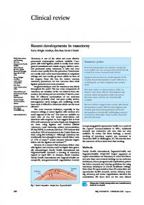
FIGURE 2. A realistic distribution for prediction errors (bottom) which is in fact a weighted combination of nine different Laplacians (top).
errors, p(e|C), within each context C, only its conditional expectation E{e|C} is estimated using the corresponding sample means e(C). ¯ These estimates are then used to further refine the prediction prior to entropy coding, by an error feedback mechanism that cancels prediction biases in different contexts. We call this process bias cancellation. The idea of gaining coding efficiency by bias cancellation arises from the observation that the conditional mean e(C) ¯ is generally not zero in a given context C. This does not contradict the well-known fact that the prediction errors without conditioning on contexts, follow a zero-mean Laplacian (symmetric exponential) distribution for most continuoustone images. The observed Laplacian distribution without conditioning on contexts is a composition of many contextsensitive distributions of different means and different variances (see Figure 2). Conditioning of the prediction error to its context provides a means to separate these distributions. Therefore, the more biased e(C) ¯ is from zero, the more effective is the process of bias cancellation. Since the conditional mean e(C) ¯ is the most likely prediction error in a given context C, we can correct the bias in the prediction by feeding back e(C) ¯ and adjusting the ˆ j] to P[i, ˜ j] = P[i, ˆ j] + e(C). prediction P[i, ¯ In order not to over-adjust the predictor, in practice the new prediction ˜ j] is estimated rather than e = error ǫ = P[i, j] − P[i, ˆ P[i, j] − P[i, j]. This in turn leads to an improved predictor ˜ j] = P[i, ˆ j] + ǫ¯ (C), where ǫ¯ (C) is the for P[i, j]: P[i, sample mean of ǫ conditioned on context C. Conceptually, bias cancellation can also be viewed as a two-stage adaptive prediction scheme via conditioning of prediction errors to contexts and the subsequent error feedback. Hence contexts used for bias cancellation are also called prediction contexts. We describe below the details by which contexts were formed and quantized by CALIC and LOCO-I1 p , the two proposals that employed bias cancellation.
where N, W, NW, NE, NN and WW are defined as in Figure 1. C is then quantized to an 8-bit binary number B = ˆ j] as the threshold, b7 b6 . . . b0 using the prediction value P[i, namely bk =
½
0 1
ˆ j] if xk ≥ P[i, ˆ j] if xk < P[i,
0 ≤ k < K = 8.
(4) Clearly, B captures the texture patterns in the modelling context which are indicative of the behaviour of the prediction error e. Also note that an event xi in a prediction context need not be a neighbouring pixel to P[i, j]. It can be a function of some neighbouring pixels. x6 and x7 , for example, represent ˆ j] forms a conthe events whether the prediction value P[i, vex or concave waveform with respect to the neighbouring pixels in the vertical and horizontal directions. Since the variability of neighbouring pixels also influences the error distribution, the texture contexts are combined with quantized error energy to form compound modelling contexts. Error energy contexts are computed by using an error energy estimator 1 defined as 1 = dh + dv + 2|ew |,
(5)
where dh and dv are as defined in Equation (1) and ew = ˆ − 1, j] (|ew | is chosen because large errors P[i − 1, j] − P[i tend to occur consecutively). 1 is then quantized to four levels yielding a quantized error energy context Q(1) which is combined with the quantized texture pattern 0 ≤ B < 2 K to form compound modelling contexts, denoted by C(δ, β). This scheme can be viewed as a product quantization of two independently treated image features: spatial texture patterns and the energy of prediction errors. At a glance, we would seemingly use 4 × 28 = 1024 different compound contexts. However, not all 28 binary codewords of the B quantizer defined by (4) are possible. By careful counting one determines that the total number of valid compound contexts is only 576 [24]. In Table 3 we show the reduction in zero-order entropy when the error feedback mechanism described above is used along with the GAP predictor. It can be seen that for some images, significant improvements can be made. On the other hand, performance can actually degrade by a little in some instances. This leads to the need for selective feedback techniques, which we are currently investigating.
T HE C OMPUTER J OURNAL, Vol. 40,
No. 2/3,
1997
132
N. M EMON AND X. W U
TABLE 3. Zero-order entropy of prediction errors with and without error feedback Image
GAP (No feedback)
GAP (with feedback)
Air1 Air2 Bike Bike3 Cafe Cats Chart Chart s Compound1 Compound2 CR CT Faxballs Finger Gold Graphic Hotel MRI Tools Ultra-Sound Water Woman X-ray
8.7669 4.8578 4.0553 4.9356 5.2469 3.5321 2.0823 3.6389 1.9934 2.1057 5.2967 4.9088 1.2951 5.6517 4.0301 2.6006 4.0132 6.2557 5.3845 3.4483 2.4834 4.5847 6.1057
8.7127 4.7518 4.0185 4.9441 5.2252 3.4818 2.0191 3.5924 2.0000 2.1114 5.2528 4.6672 1.2344 5.5077 4.0045 2.5093 3.9475 6.1720 5.3966 3.4086 2.4439 4.5485 6.0629
Average
4.229
4.174
P(e|q1 , q2 , q3 , q4 ) = P(−e|−q1 , −q2 , −q3 , −q4 ). The total number of contexts turns out to be 1094 within each of which the bias in prediction error is estimated in a manner similar to CALIC. Extensive evaluation of the two context formation and quantization techniques described above showed little difference in compression performance for typical images. The second set of techniques was adopted by the committee for the proposed standard since it is simpler. In fact it was simplified further before adoption in the final committee draft of the standard by dropping the difference D4 and thereby obtaining a reduced context count of 364 [5]. 5. COMPUTING CODING CONTEXTS
4.2. Context formation and quantization in LOCO-I1p Inspired by the success of the CALIC algorithm in the first round of evaluations, the HP group submitted a significantly different algorithm [7] which was one-pass (as opposed to their original two-pass submission [6]) and incorporated the context-based bias cancellation mechanism proposed in CALIC. However, they considerably simplified the context formation and quantization techniques and combined them with a very simple and efficient entropy coding technique (described in Section 6), while obtaining compression ratios that were only 3% inferior to CALIC’s on a majority of ISO test images. Contexts in LOCO-I1 p are formed by first computing the following differences: D1 = NE − N D2 = N − NW D3 = NW − W D4 = WW − W.
based on the assumption that
As mentioned earlier in Section 2, in practice it is observed that prediction does not completely remove the statistical redundancy in the image even after context-based bias cancellation. The variance of prediction errors strongly correlates to the smoothness of the image around the predicted pixel P[i, j]. To model this correlation predictive techniques usually condition the encoding of the prediction error on local image activity level and on quantized prediction errors incurred in neighbouring pixels. However, a direct implementation of this approach, due to the large number of conditioning states or contexts and the large alphabet size of prediction errors, faces two major difficulties: the use of prohibitively large memory space for error modelling, and the lack of sufficient samples in each context during adaptive coding in order to make reliable probability estimations. Reducing the number of contexts could be one way to address this problem. Many of the lossless compression techniques reported in the literature have adopted this approach and use only a small number of contexts for conditioning the encoding of prediction errors. However, this leads to poorer performance due to loss in modelling efficiency. Another key contribution of the CALIC proposal was a modelling paradigm that employed a large number of contexts for bias cancellation, but merged the bias cancellation contexts into a few conditioning states for entropy coding of errors. These conditioning states are also called coding contexts in order to distinguish them from bias cancellation contexts. 5.1.
(6)
The differences D1, D2 and D3 are then quantized into nine regions (labelled −4 to +4) symmetric about the origin with one of the quantization regions (region 0) consisting of only the difference value 0. The difference D4, being further away from the current pixel, is quantized into only three regions (labelled −1 to +1). Furthermore, contexts of the type (q1 , q2 , q3 , q4 ) and (−q1 , −q2 , −q3 , −q4 ) are merged
Coding contexts in CALIC
Coding contexts in CALIC were computed by first computing an error energy estimator 1 as defined in (5). Conditioning the error distribution on 1 leads to separation of prediction errors into classes of different variances. Thus entropy coding of errors using estimated conditional probability p(e|1) improves coding efficiency over using p(e). For time and space efficiency, 1 has to be quantized to a small number of (L) levels. In practice, L = 8 is found to be sufficient. Larger L only improves coding efficiency marginally. Although the 1 quantizer Q(1) can be optimized off-line
T HE C OMPUTER J OURNAL, Vol. 40,
No. 2/3,
1997
L OSSLESS I MAGE C OMPRESSION TABLE 4. Entropy of prediction errors before and after conditioning on coding contexts
Image
GAP No conditioning
GAP Conditioned on Q(1)
Air1 Air2 Bike Bike3 Cafe Cats Chart Chart s Compound1 Compound2 CR CT Faxballs Finger Gold Graphic Hotel MRI Tools Ultra-Sound Water Woman X-ray
8.7127 4.7518 4.0185 4.9441 5.2252 3.4818 2.0191 3.5924 2.0000 2.1114 5.2528 4.6672 1.2344 5.5077 4.0045 2.5093 3.9475 6.1720 5.3966 3.4086 2.4439 4.5485 6.0629
8.5940 4.1220 3.5995 4.4508 4.7753 2.5518 1.4355 2.8957 1.4742 1.4550 5.1861 4.0546 1.0241 5.4989 3.8731 2.3658 3.7738 5.9331 5.0437 2.7810 1.8202 4.1098 5.9305
Average
4.174
3.772
133
estimation context, which is computed as described in Subsection 4.2. This is done by maintaining in each context, the count N of the prediction errors seen so far and the accumulated sum of magnitudes of prediction errors A seen so far. The coding context k is then computed as ′
k = min{k ′ |2k N ≥ A}. The reason for doing this is tied in to the specific entropy coder that LOCO-I1 p uses, which is described in the next section. The strategy employed is an approximation to the optimal parameter selection for this entropy coder. For details the reader is referred to [6, 7]. 5.3.
Coding contexts in ALCM and JSLUG
Coding contexts in the ALCM proposal were obtained by quantizing the maximum prediction error in the four nearest neighbours of the current pixel. This maximum error was quantized into seven levels using fixed thresholds in order to form seven coding contexts in which adaptive binary arithmetic coding was performed. The JSLUG proposal, on the other hand, quantizes the prediction errors incurred in the North, West and NorthEast neighbours into 7, 7 and 3 levels respectively, yielding 147 contexts in which adaptive binary arithmetic coding is performed. Some binary decisions are encoded conditioned on the sign of the current prediction error after it has been revealed and thus utilize 147 × 2 = 294 contexts. 6. ENTROPY CODING
by standard dynamic programming techniques in order to minimize the conditional entropy of prediction errors over a training set of images [24], in practice, it was found that an image-independent 1 quantizer with bins which are fixed, q1 = 5, q2 = 15, q3 = 25, q4 = 42, q5 = 60, q6 = 85, q7 = 140,
(7)
worked almost as well as the optimal image-dependent 1 quantizer. Estimating L = 8 conditional error probabilities p(e|Q(1)) requires only a modest amount of memory while estimating probabilities for entropy coding. Furthermore, the small number of conditional error probabilities involved means that even small images will provide enough samples to learn p(e|Q(1)) quickly to facilitate an adaptive entropy coding technique. In Table 4 we list the zero-order entropy of prediction errors using the GAP predictor and the entropy after conditioning on the coding contexts described above. It can be clearly seen that significant improvement is obtained. 5.2. Coding contexts in LOCO-I1p LOCO-I1 p uses k-coding contexts for a k bit/pixel image. The specific coding context is computed from the expected magnitude of the prediction error within the current bias
An advantage of the techniques that employ prediction followed by error modelling is the clean separation between prediction, modelling of prediction errors, and entropy coding of prediction errors. Quite often, any entropy coder, be it Huffman or arithmetic, static or adaptive, binary or m-ary, can usually be interfaced with such a system. Considering this fact, a variety of entropy coding techniques was proposed including Huffman coding, m-ary and binary arithmetic coding and Golomb–Rice coding. The main contribution came from the HP group’s revised LOCO-I1 p proposal in the form of an ingeniously simple and effective usage of Golomb–Rice coding. In the rest of the section we briefly describe some of the coding techniques that were proposed in the CALIC, LOCO and ALCM proposals. 6.1.
Entropy coding in the CALIC system
CALIC used an adaptive m-ary arithmetic coder, CACM++ package that was developed and made publicly available by Carpinelli and Salamonsen. The software is based on the work in [25]. The compression results that we report in the next section were obtained by coupling CALIC with CACM++. However, CALIC does not feed an m-ary arithmetic coder with prediction errors directly. Instead it first remaps prediction errors into an alphabet of size 2z
T HE C OMPUTER J OURNAL, Vol. 40,
No. 2/3,
1997
134
N. M EMON AND X. W U
instead of 2z+1 for a z-bit image. Also, the tails of error distributions are truncated and an escape mechanism is used to further reduce the number of code symbols. The actual bit rates achieved are mostly very close and sometimes even better than the corresponding entropy figures. 6.2. Entropy coding in the LOCO-I1p system In LOCO-I1 p the prediction errors are encoded using a special case of Golomb codes [26] which is also known as Rice coding [27]. Golomb codes of parameter m encode a positive integer n by encoding n mod m in binary followed by an encoding of n div m in unary. When m = 2k the encoding has a very simple realization and has been referred to as Rice coding in the literature. For an image with z bits/pixel, prediction errors can be mapped to the range 0 to 2z − 1 and the coding parameter k can vary from 0 to z − 1. However, instead of attempting codes with each parameter on a block of symbols and selecting the one which results in the shortest code [27], in LOCO-I1 p , the coding parameter k is estimated on the fly for each prediction error. We have briefly described this parameter estimation procedure in Subsection 4.2 and for details the reader is referred to [7]. Despite the simplicity of the coding and estimation procedures, the compression performance achieved is surprisingly close to that obtained by arithmetic coding.
TABLE 5. Bit rates (bits/pixel) of some proposed schemes on ISO test set and comparison with lossless JPEG (Huffman). Note that averages were only taken over those images with no missing entries in any column. Image
CALIC
LJPEG
LOCO-I1 p
ALCM
Air1 Air2 Bike Bike3 Cafe Cats Chart Chart s Compound1 Compound2 CR CT Faxballs Finger Gold Graphic Hotel MRI Tools Ultra-Sound Water Woman X-ray
8.31 3.83 3.50 4.23 4.69 2.51 1.28 2.66 1.24 1.24 5.17 3.63 0.75 5.47 3.83 2.26 3.71 5.73 4.95 2.34 1.74 4.05 5.83
– 4.90 4.33 5.15 5.63 3.69 2.23 3.86 2.51 2.50 – – 1.50 5.85 4.22 2.81 4.22 – 5.69 3.63 2.62 4.84 –
8.50 4.00 3.59 4.37 4.80 2.59 1.33 2.74 1.30 1.35 5.27 3.84 0.98 5.63 3.92 – 3.78 6.04 5.07 2.67 1.79 4.18 5.97
8.77 4.08 3.69 4.43 4.99 2.67 1.27 2.77 1.29 1.34 5.43 4.09 0.60 5.94 4.02 2.41 3.92 6.17 5.17 2.32 1.82 4.30 6.24
Average
3.06
3.96
3.18
3.21
6.3. Entropy coding in the ALCM system The ALCM and JSLUG proposals used adaptive binary arithmetic coding to encode prediction errors within each coding context. Since binary coding is used the prediction error needs to be binarized before encoding. In ALCM, prediction errors are first mapped to the range 0 to 2z − 1 and then binarized using a decision tree. A separate binary decision tree is maintained for each of the seven coding contexts and the first binary decision encoded is whether the symbol is more or less than a parameter value m. If the symbol is greater m is subtracted and the procedure repeated until a negative branch is taken. In this case the binarization is done by a decision tree for m equally probable symbols; essentially, the procedure involves adaptive binary arithmetic coding of the Golomb m code of the prediction error. Different values of m are used for each coding context. For simplicity of implementation m is always a power of 2. 6.4. Overall compression performance results In Table 5 we show final bit rates that were reported by the CALIC, LOCO-I1 p and the ALCM proposals. The bit rates shown are after a few additional tricks that were used by each technique to improve compression performance. For example, the CALIC proposal included a sign prediction technique for reducing the conditional entropy of prediction errors. Also, both CALIC and LOCO-I1 p included alphabet extension mechanisms for low-entropy images or regions where it is potentially beneficial to encode runs of uniform
symbols. For these reasons the bit rates for CALIC in Table 5 are lower than the corresponding rates in Table 4. The reader is referred to the original proposals for details. Also included in the table are bit rates obtained by a publicly available lossless JPEG implementation of Cornell University (LJPEG). One can see from the results that the three proposed algorithms listed significantly outperform the current lossless standard. Although CALIC gives the best overall performance, the bit rates of LOCO-I1 p are remarkable, given its simplicity. The baseline algorithm that has been finalized is essentially the one given in LOCO-I1 p with minor modifications. 7. CONCLUSION AND AVENUES FOR FUTURE WORK The standardization project for lossless image compression of continuous-tone images has resulted in significant advances in the state of the art of such techniques. In this paper we briefly surveyed some of the key ideas that emerged in the process. One of these was CALIC’s modelling paradigm that uses a large number of contexts to estimate conditional prediction biases, and compensates for such biases through an error feedback mechanism. This approach offers an effective means of reducing model cost, a vital issue in lossless image coding, by using a large number of contexts for bias
T HE C OMPUTER J OURNAL, Vol. 40,
No. 2/3,
1997
L OSSLESS I MAGE C OMPRESSION cancellation but merging these contexts into a few contexts for conditional entropy coding of prediction errors. The second, and perhaps most important key contribution was the ingenious and effective technique of Golomb–Rice coding using sequential parameter estimation in the revised HP proposal, LOCO-I1 p . In spite of being extremely simple to implement both in software and hardware, the coding performance comes within a few per cent of much more complex arithmetic-coding-based techniques. Another key observation that emerged in the convergence process was the efficacy of the MED predictor used in the LOCO submissions. Although the MED predictor has been known for a long time, its effectiveness for prediction in lossless image compression had not been realized. In fact, it is interesting to ask why MED yields such good performance. In addition, the simple context formation and quantization mechanisms presented in the LOCO proposals were also important contributions and were adopted into the baseline standard. We have reported the recent advances in lossless image coding. For both theoretical and practical interests one would like to know how much gap still exists between the lossless bit rates obtainable by the new JPEG lossless standard and the ultimate image compressibility regardless of computational complexity. The question becomes even more tantalizing considering that the best (also the most expensive) version of CALIC [23] has reached a 2% shorter average code length than the universal context modelling (UCM) algorithm [6, 7]. The latter is a highly complex but principled algorithm with a provable asymptotical optimality in compressibility. A recent study [23] seemed to suggest that the ratio of compression gains versus computational complexity is diminishing. We can identify two possible problems that may prevent further improvement in coding efficiency: (i) there may exist undiscovered structures of prediction errors associated with some events other than the local intensity gradients and neighbouring errors which have already been exploited by the current methods, and (ii) the context quantizers employed by the current methods may deviate significantly from an optimal error classifier that minimizes conditional entropy. ACKNOWLEDGEMENTS The authors would like to thank the reviewers for their substantive and informed review which led to significant improvements in the manuscript. N. M. was partially supported by NSF Career award NCR 9703969. REFERENCES [1] Langdon, G. G. (1991) Sunset: a hardware oriented algorithm for lossless compression of gray scale images. In Medical Imaging V: Image Capture, Formatting and Display, Vol. 1444, pp. 272–282. SPIE. [2] Howard, P. G. and Vitter, J. S. (1993) Fast and efficient lossless image compression. In Storer, J. A. and Cohn, M. (eds), Proc. Data Compression Conf., pp. 351–360. IEEE Computer Society Press, Los Alamitos, CA.
135
[3] Tischer, P. E., Worley, R. T., Maeder, A. J and Goodwin, M. (1993) Context-based lossless image compression. Comp. J., 36, 68–77. [4] ISO/IEC JTC 1/SC 29/WG 1 (1994) Call for contributions— lossless compression of continuous-tone still pictures. ISO Working Document ISO/IEC JTC1/SC29/WG1 N41. [5] ISO/IEC JTC 1/SC 29/WG 1 (1997) CD 14495, Lossless and near-lossless compression of continuous-tone still images (JPEG-LS). ISO Working Document ISO/IEC JTC1/SC29/WG1 N522. [6] Weinberger, M. J., Seroussi, G. and Sapiro, G. (1995) LOCOI: a low complexity lossless image compression algorithm. ISO Working Document ISO/IEC JTC1/SC29/WG1 N203. [7] Weinberger, M. J., Seroussi, G. and Sapiro, G. (1995) LOCOI: new developments. ISO Working Document ISO/IEC JTC1/SC29/WG1 N245. [8] Howard, P. G. and Vitter, J. S. (1992) Error modeling for hierarchical lossless image compression. In Storer, J. A. and Cohn, M. C. (eds), Proc. Data Compression Conf., pp. 269– 278. IEEE Computer Society Press, Los Alamitos, CA. [9] Rissanen, J. J. and Langdon, G. G. (1981) Universal modeling and coding. IEEE Trans. Inform. Theory, IT-27, 12–22. [10] Todd, S., Langdon, G. G. and Rissanen, J. J. (1985) Parameter reduction and context selection for compression of gray scale images. IBM J. Res. Develop., 29, 188–193. [11] Pennebaker, W. B. and Mitchell, J. L. (1993) JPEG Still Image Data Compression Standard. Van Rostrand Reinhold, New York. [12] Boliek, M. and Zandi, A. (1995) CREW: lossless/lossy image compression—contribution to ISO/IEC JTC 1.29.12. ISO Working Document ISO/IEC JTC1/SC29/WG1 N196. [13] Mochizuki, T. (1995) Proposal for lossless compression of continuous-tone still pictures: lossless transform coding for still pictures (LTC). ISO Working Document ISO/IEC JTC1/SC29/WG1 N196. [14] Urban, S. (1995) Compression results—lossless, lossy ±1, lossy ±3. ISO Working Document ISO/IEC JTC1/SC29/WG1 N281. [15] Martucci, S. A. (1990) Reversible compression of HDTV images using median adaptive prediction and arithmetic coding. In IEEE Int. Symp. on Circuits and Systems, pp. 1310–1313. IEEE Press, New York. [16] Memon, N. D. and Sayood, K. (1995) Lossless image compression—a comparative study. In Still Image Compression, SPIE Proc., Vol. 2418, pp. 8–20. [17] Wu, X., Memon, N. D. and Sayood, K. (1995) A contextbased, adaptive, lossless/nearly-lossless coding scheme for continuous-tone images. ISO Working Document ISO/IEC/ SC29/WG1/N256. [18] Speck, D. (1995) Proposal for next generation lossless compression of continuous-tone still pictures: activity level classification model (ALCM). ISO Working Document ISO/IEC JTC1/SC29/WG1 N198. [19] Langdon, G. G., Speck, D., Haidinyak, C. and Macy, S. (1995) Contribution to JTC 1.29.12: JSLUG. ISO Working Document ISO/IEC JTC1/SC29/WG1 N199. [20] Memon, N. D., Sippy, V. and Wu, X. (1996) A comparison of the prediction schemes proposed for a new standard on lossless coding of continuous-tone still images. In Proc. ISCAS 96, pp. II-309–312. IEEE Press, New York. [21] Ueno, I. and Ono, F. (1995) CLARA: continuous-tone lossless coding with edge analysis and range amplitude detection. ISO Working Document ISO/IEC JTC1/SC29/WG1 N197.
T HE C OMPUTER J OURNAL, Vol. 40,
No. 2/3,
1997
136
N. M EMON AND X. W U
[22] Gandhi, B., Honsinger, C., Rabbani, M. and Smith, C. (1995) A proposal submitted in response to call for contributions for JTC 1.29.12 [JTC1/SC29/WG1 N41] ISO Working Document ISO/IEC JTC1/SC29/WG1 N204. [23] Wu, X. (1997) Efficient and effective lossless compression of continuous-tone images via context selection and quantization. IEEE Trans. Image Processing, IP-6, 656–664. [24] Wu, X. and Memon, N. D. (1997) Context-based adaptive lossless image coding. IEEE Trans. Commun., 45, 437–444.
[25] Moffat, A., Neal, R. and Witten, I. (1995) Arithmetic coding revisited. In Proc. Data Compression Conf., pp. 202–211. [26] Golomb, S. W. (1966) Run-length codings. IEEE Trans. Inform. Theory, IT-12, 399–401. [27] Rice, R. F. (1979) Some Practical Universal Noiseless Coding Techniques. Technical Report 79-22, Jet Propulsion Laboratory, California Institute of Technology, Pasadena, CA.
T HE C OMPUTER J OURNAL, Vol. 40,
No. 2/3,
1997