COLLEGE OF ENGINEERING ... not discuss applications to computational mechanics in general and finite element methods in ...... As a result, it is still the best.
CU-CAS-96-03
CENTER FOR AEROSPACE STRUCTURES
RECENT DEVELOPMENTS IN PARAMETRIZED VARIATIONAL PRINCIPLES FOR MECHANICS
by C. A. Felippa
January 1996
COLLEGE OF ENGINEERING UNIVERSITY OF COLORADO CAMPUS BOX 429 BOULDER, COLORADO 80309
Recent Developments in Parametrized Variational Principles for Mechanics
Carlos A. Felippa Department of Aerospace Engineering Sciences and Center for Aerospace Structures University of Colorado, Boulder CO 80309-0429, USA
January 1996
Report No. CU-CAS-96-03
Paper contributed for the 10th anniversary volume of Computational Mechanics Published in Vol 11, 443–461, 1996.
RECENT DEVELOPMENTS IN PARAMETRIZED VARIATIONAL PRINCIPLES FOR MECHANICS
Carlos A. Felippa Department of Aerospace Engineering Sciences and Center for Aerospace Structures University of Colorado, Boulder Boulder, CO 80309-0429, USA
Abstract. This paper gives an introduction to the formulation of parametrized variational principles (PVPs) in mechanics. This is complemented by more advanced material describing selected recent developments in hybrid and nonlinear variational principles. A PVP is a variational principle containing free parameters that have no effect on the Euler-Lagrange equations and natural boundary conditions. The theory of single-field PVPs, based on gauge functions, is a subset of the Inverse Problem of Variational Calculus that has limited value. On the other hand, multifield PVPs are more interesting from both theoretical and practical standpoints. The two-dimensional Poisson equation is used to present, in a tutorial fashion, the formulation of parametrized mixed functionals. This treatment is then extended to internal interfaces, which are useful in treatment of discontinuities, subdomain linkage and construction of parametrized hybrid functionals. This is followed by a similar but more compact treatment of three-dimensional classical elasticity, and a parametrization of nonlinear hyperelasticity.
1. Introduction This paper introduces basic concepts behind the formulation of parametrized variational principles (PVPs) in mechanics. This is complemented by more advanced material describing recent developments made since the publication of a comprehensive survey (Felippa 1994). Most of the introductory exposition is taken from that reference. For reasons of space the present article does not discuss applications to computational mechanics in general and finite element methods in particular. Such applications are summarized in that survey and elaborated in the references given therein. A PVP derives from a functional with free parameters if the Euler-Lagrange equations and natural boundary conditions turn out to be independent of those parameters. It is useful to emphasize the distinction between single-field PVPs, in which only one primary field is varied, and multifield (mixed or hybrid) PVPs. Single-field PVPs have been extensively studied but lack interest for applications. Multifield PVPs are less understood but are far more interesting from the dual standpoint of theory and applications. The present study of multifield PVPs was originally motivated by the desire of finding a variational framework for finite elements based on the Free Formulation of Bergan and Nyg˚ard (1984), later expanded to the Scaled Free Formulation of Bergan and Felippa (1985). In numerical tests those elements had displayed excellent performance, but a theoretical explanation was lacking. This foundation was provided by parametrized functionals (Felippa 1989). As sometimes happens, this modest goal led to unexpected discoveries, chief among them a general parametrization of the functionals of classical elasticity (Felippa and Militello 1989, 1990). Subsequently more applications to finite elements were revealed. 2. Basic Concepts and Definitions 2.1 Some Simple Examples Beginner calculus students are soon taught about the presence of an integration constant when obtaining indefinite integrals of functions of one variable: � dy = F(x), y(x) = F(x) d x = G(x) + C, (1) dx where G(x) is a primitive of F(x). Later on, in multivariable calculus they learn about partial integrals: � ∂z = F(x, y), z(x, y) = F(x, y) d x = G(x, y) + C(y). (2) ∂x The fact that primitive functions are not unique, because differentiation is a restricting operation, can be viewed as the simplest example of parametrized functionals. As a next example consider a single-field functional �(u) that depends on a function u(x) of a single spatial variable that satisfies appropriate smoothness requirements. The functional � also contains a free parameter β: � b � b � � 1 1 −(u � )2 + 2βuu � + u 2 d x, (3) F(u; β) d x = 2 �(u; β) = 2 a
a
1
where primes denote derivative with respect to x. The Euler-Lagrange equation associated with δ� = 0 is (4) E(u) = u �� + u = 0, which is independent of β. The natural boundary conditions � � ∂ F �� ∂ F �� � = βu(a) − u (a) = 0, = βu(b) − u � (b) = 0, ∂u � � ∂u � � x=a
(5)
x=b
are not independent of β unless u(a) = u(b) = 0. The parameter-independence of the EulerLagrange equation and natural boundary conditions characterize parametrized variational principles, which are defined more precisely in Section 2.3. The example can be generalized with arbitrary functions by replacing βuu � with β(Pu � + Q), where P and Q are functions of u and x only, as shown in the next subsection. 2.2 Principal and Gauge Functionals The explanation for the behavior of the preceding functionals is straightforward. Consider (3) in which the parametrized term is split as � � P (u) =
1 2
a
�(u; β) = � P (u) + β �G (u), � b b� � � � � 2 2 −(u ) + u d x, �G (u) = uu � d x = 12 u 2 (b) − u 2 (a) .
(6) (7)
a
Here � P is labeled as the principal functional whereas �G is labeled as a gauge functional. The latter is also called a null Lagrangian in the literature. Because �G depends only on boundary values, its contribution to the Euler-Lagrange equation of � is obviously zero; thus cancelling the effect of β. The converse statement is also a well known theorem of variational calculus: if the Euler-Lagrange equation of a single-field functional containing up to first-order derivatives vanishes identically, that functional must depend only on boundary values. For a scalar function of one variable the proof is short. The Euler-Lagrange equation of a gauge functional FG (u) depending on u(x) and u � (x) is � � d ∂ FG ∂ 2 FG ∂ 2 FG � ∂ 2 FG �� ∂ FG ∂ FG − − − u − u ≡ 0. (8) = ∂u d x ∂u � ∂u ∂ x∂u � ∂u∂u � ∂u � ∂u � If (8) is an identity for any FG , the function coefficient of u �� must vanish; thus FG must be of the form Pu � + Q, where P and Q are functions of u and x. Substitution into (8) yields ∂ Q/∂u = ∂ P/∂ x, which shows that P du + Q d x must be the exact differential of a function G(u, x). Consequently � FG (u) d x = G(u, x) and the value of the integral depends only on its end points. This result is easily generalized to vector functions u(x)T = {u 1 (x), . . . , u n (x)} . These are particularly relevant to semi-discrete dynamical systems with n degrees of freedom, in which x becomes the time t. Should the single-field functional depend on several independent variables x, y, . . ., one can obviously add the divergence or curl of multidimensional functions multiplied by free parameters, because application of Green’s or Stokes’ theorems reduces such functions to boundary terms. If the functional depends on derivatives of higher order than first, the situation becomes more complicated; that case is studied in Chapter IV of the textbook by Courant and Hilbert (1953). 2
VF
The Inverse Problem
Homogenize variations and integrate Perform variation(s) and homogenize
Enforce all relations pointwise
SF
WF
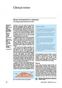
Weaken selected relations Figure 1. Diagram sketching Strong, Weak and Variational Forms, and relationships between form pairs. (Weak Forms are also called weighted-residual equations, variational equations, Galerkin equations and integral statements in the literature.)
2.3 Terminology A functional that contains one or more free parameters, such as � in the foregoing example, is called a parametrized functional. If its Euler-Lagrange equation and natural boundary conditions are independent of the parameters, then the stationarity condition δ� = 0 is called a parametrized variational principle or PVP. A PVP is most useful from the standpoint of applications if the value of the functional, evaluated at an extremal, is independent of the free parameters. This value has often the meaning of energy. Such a principle will be called an invariant parametrized variational principle or IPVP. The example functional (3) yields an IPVP if, in addition to u(a) = u(b) = 0, [u �� (b)]2 = [u �� (a)]2 or if [u � (b)]2 = [u � (a)]2 . (To prove the latter, insert u = −u �� into �G and integrate.) The condition for a PVP to be invariant can be generally expressed through Noether’s conservation-law theorem of variational calculus; see for instance Sec. 20 of Gelfand and Fomin (1963). But for many cases that kind of invariance can be checked directly. The most useful invariant PVPs are those in which invariance does not depend on boundary conditions. Such functionals will be encountered in Sections 4 and 6.
3
2.4 Connections with the Inverse Problem The study of single-field PVPs constitutes a subset of the Inverse Problem of Variational Calculus: given a system of ordinary or partial differential equations — herein called the Strong Form or SF — find the Lagrangians that have that system as Euler-Lagrange equations. These Lagrangians, if they exist, collectively embody the Variational Form (VF) of the problem. The Weak Form (WF), which is also known by the alternative names listed in Figure 1, is an intermediary between SF and VF. Relations between those forms are annotated in that Figure. The Inverse Problem linking ordinary differential equations to single-field functionals is treated in several monographs (e.g., Santilli 1979; Sewell 1987; Vujanovic and Jones 1989). On the other hand, the multifield case is less developed, particularly in the case of multiple space variables. 2.5 Theoretical and Practical Advantages PVPs are interesting from a theoretical standpoint because of their unifying value: a single PVP is equivalent to a family of functionals. Specific functionals can be obtained by setting parameters to specific values. A theorem proved for a PVP is “economical” in the sense that it need not be redone for specific cases. Books and articles on the variational formulations of field problems for physics and engineering usually focus on the so-called canonical functionals, which are those found to be either of substantial practical value, or historical interest. Examples of these are the Minimum Potential Energy, Hellinger-Reissner and Hu-Washizu functionals of classical elasticity. That kind of presentation has two drawbacks. First, what ought to be shared properties are proved over and over, a feat that can result in voluminous expositions. Second, readers may be left with the impression that only a limited number of functionals for say, elasticity, have been discovered, which encourages the publication of “new” functionals in an nonending stream of articles. The main interest of PVPs, in the applications, center on direct methods that use variational principles as a source of analytical or numerical approximations. Chief among the latter is the Finite Element Method (FEM). The key observation is that approximations depend on the free parameters. On the other hand, the converged solution, assuming a convergent discretization method, does not. Thus an obvious question arises: can the free parameters be chosen in such a way that errors are minimized while the number of degrees of freedom remain modest? An implementation of this idea in the FEM arena leads to High Performance Elements and templates (Felippa 1994). Additional information on these research thrusts is given in the Conclusions section. 3. A Two-Field 1-D Example As our first encounter with a multifield PVP, the following 6-coefficient generalization of (3) to two independently varied fields: u and p = u � , is postulated: � �(u, p ; J) = a
b
�
F(u, u , p) d x =
� 1 2
a
b
u u� p
T
4
j11 j12 j13
j12 j22 j23
j13 j23 j33
u u� p
� dx =
1 2
b
zT Jz d x, a
(9)
: d ∪ q
�
y
n
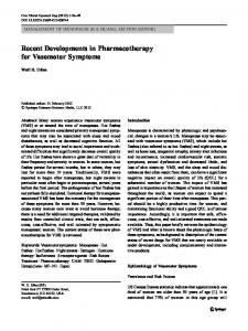
x Figure 2. Two-dimensional region for isotropic Poisson equation (13).
in which
j11 j12 j13 u J = j12 j22 j23 . (10) z = u� , p j13 j23 j33 are the generalized field vector and the functional generating matrix, respectively. This parameter matrix — the “kernel” of the quadratic form in the z vector — may be taken as symmetric because only its symmetric part participates in the first variation. This general notational arrangement is followed in more complicated linear problems of mathematical physics presented later.
The Euler-Lagrange equations supplied by δu � = 0 and δ p � = 0 are d Fu � = j11 u + j12 u � + j13 p − ( j12 u � + j22 u �� + j23 p � ) = 0, dx d F p� = j13 u + j23 u � + j33 p = 0. E p : Fp − dx E u : Fu −
(11)
Consistency of E p and E u with the field equations u � − p = 0 and u + p � = 0, respectively, dictates that J be of the form
α β 0 J= β (12) 0 −α . 0 −α α Thus �(u, p) is found to depend on two independent free parameters: α and β. The one-field functional (3) is recovered if the “strong connection” p = u � is enforced a priori and α = 1. The parametric independence of natural boundary conditions, however, imposes additional constraints on α and β unless appropriate boundary terms are added to �. In the next example such terms appear naturally from the beginning.
5
4. A Three Field Example: the 2-D Poisson Equation 4.1 Problem Description As an example which is more typical of practical applications, we develop an invariant PVP for the 2-D isotropic Poisson equation (the Laplace equation with a source term). This PDE is posed over a finite two-dimensional region � bounded by a curve , as illustrated in Figure 2: � 2 � ∂ u ∂ 2u 2 + 2 =−f in �, (13) k∇ u = k ∂x2 ∂y where u = u(x, y) is the unknown primary function, k(x, y) > 0, and f (x, y) is a given scalar function in �. The physical meaning of this equation is left unspecified. In technical applications, however, u may stand for such diverse field quantities as temperature, fluid pressure, Prandtl’s torsion stress function, or electrostatic potential. [For non-isotropic problems k must be replaced by a 2 × 2 constitutive matrix S and (13) becomes ∇ T S ∇ u = − f , but the underlying framework is unchanged.] The boundary is decomposed into d ∪ q , on which the following Dirichlet and Neumann (flux-type) boundary conditions, respectively, are imposed: u = dˆ
on
d ,
k
∂u = k (grad u)T n = qˆ ∂n
on
q ,
(14)
where dˆ and qˆ are prescribed on u and q , respectively, and n is the exterior unit normal on . It should be noted that dˆ is used instead of u, ˆ which seems a more logical notation for prescribed values, to link up smoothly with “functional hybridization” in Section 5. For such developments it will be convenient to notationally distinguish the interior field u from the boundary field d. The single-field functional �(u) associated with (13) and (14) is well known: � = U (u) − P(u) where
�
� U (u) =
1 2
k �
∂u ∂x
�
�2 +
∂u ∂y
�2
(15) �
� d�,
P(u) =
�
f u d� +
q
qˆ u d ,
(16)
in which u satisfies strongly the Dirichlet B.C. u = dˆ on d . In this functional U (u) has the meaning of internal energy, whereas P(u) is an external energy associated with the source and prescribednormal-flux terms f and q. ˆ As previously noted, functional (15) can be trivially parametrized by adding multiples of the divergence or curl of gauge functions. But such PVPs have no practical importance. To allow the construction of a multifield PVP we introduce the two vector fields: gradient g and flux vector p, as candidates for independent variation: � � � � ∂u/∂ x px ∂u/∂ x gx = grad u = , p= = kg = k grad u = k . (17) g= gy py ∂u/∂ y ∂u/∂ y 6
dˆ
u = dˆ
f
u
on d
div p + f = 0 in �
g = grad u in � p=kg
g
pn = qˆ
p
in �
Unknown field
on q
qˆ
Data field
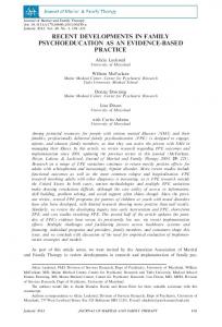
Strong connection Figure 3. Graphical representation of the Strong Form (SF) of the isotropic two-dimensional Poisson equation (13) with the B.C.s (14) as a modified Tonti diagram.
The second order PDE (13) decomposes into the three field equations g = ∇u = grad u,
p = k g,
∇ T p + f = div p + f = 0,
(18)
where div ≡ ∇ T is the divergence operator. In mechanical applications (18) are called the kinematic, constitutive and balance (or equilibrium) equations, respectively. The projection of the flux p on a unit normal n to some curve is called the normal flux and denoted by pn = pT n. Hence the boundary conditions (14) may be compactly stated as u = dˆ
on
d ,
pn = qˆ
on
q .
(19)
The three field equations (18) and two boundary conditions (19) collectively make up the Strong Form (SF) of the isotropic Poisson equation. This SF is graphically represented in Figure 3 using a modified Tonti diagram. Relations such as g = grad u are called strong connections (which means that they are enforced point by point) and depicted as solid lines. The main departure of Figure 2 from Tonti’s original diagrams (Tonti 1973; Oden and Reddy 1982) is the explicit separation of field equations and boundary conditions; this has been found useful in teaching variational methods. In addition, a graphical distinction is made between unknown and data fields, as indicated in Figure 3, also for instructional reasons. A variational form (VF) substitutes one or more strong connections by weak ones. For example the functional �(u) defined by (15) and (16) weakens the equilibrium equations and Neumann boundary conditions, and may be graphically represented as shown in Figure 4. More general forms are constructed in the following subsection. 7
dˆ
u = dˆ on d
�
g = grad u in �
;;;
;; ;;;; f
u
�
(div p + f ) δu d� +
�
g
p=kg in �
q
=0
( pn − q) ˆ δu d
p
qˆ
Weak connection (for other symbols, cf. Figure 3)
Figure 4. Graphical representation of the single-field Variational Form (15)-(16) as a modified Tonti diagram.
4.2 A Three-Field PVP for Poisson Equation The configuration of (16) suggests trying to parametrize the internal energy U as a three-field quadratic form, leading to the arrangement displayed below in full: T −1 px j11 j11 j12 j12 j13 j13 k px −1 p j j j j j j k py y � 11 11 12 12 13 13 kgx j12 j12 j22 j22 j23 j23 gx 1 (20) U (u, p, g) = 2 d�, kg y j12 j12 j22 j22 j23 j23 g y � k ∂u/∂ x j13 j13 j23 j23 j33 j33 ∂u/∂ x j13 j13 j23 j23 j33 j33 k ∂u/∂ y ∂u/∂ y in which, for simplicity, the explicit dependence of U on the j coefficients is dropped from its arguments. The symmetry of the kernel matrix can be justified by inspection, whereas its 2 × 2 block structure is a consequence of avoiding distortions in the vector-component contributions to the internal energy. This functional is fully specified if the 3 × 3 generating matrix J, which has the same form as in (10), is given. Now, Eq. (20) looks unduly complicated for such a simple problem. At the same time, what is being varied is not easily seen. We clarify and simplify this form in two steps: passing to matrix-vector notation, and then applying the primary- versus derived-field convention, as explained below:
−1
T � k p˜ p˜ j11 I j12 I j13 I ˜ = 12 d� U (u, ˜ g˜ , p) j12 I j22 I j23 I k g˜ g˜ � k grad u ˜ grad u˜ j13 I j23 I j33 I (21)
T p � g p˜ j11 I j12 I j13 I = 12 pg j12 I j22 I j23 I g˜ d�. � pu j13 I j23 I j33 I gu 8
Here I denotes the 2×2 identity matrix, pg = k g˜ , pu = k gu = k grad u, ˜ g p = k −1 g˜ , gu = grad u. ˜ This notational convention, introduced in (Felippa 1989), is based on two rules: 1.
˜ This allows one to A varied (primary) field is marked with a superposed tilde such as u˜ or p. reserve tildeless symbols such as u or p for generic or exact fields. The tilde may be omitted where variation is evidently implied; for instance δu is obviously the same as δ u. ˜
2.
A derived (secondary) field is identified by writing its “parent” primary field as superscript; ˜ for example pu = k grad u˜ is the flux associated with the varied field u.
Of course at the exact solution of (13), all p’s and g’s coalesce, but the distinction is crucial in variational-based approximation methods. Note the pleasing appearance of the last term in (21): the notation groups fluxes on the left and gradients on the right. Flux times gradient is internal energy density, so the kernel matrix simply weights, through the j coefficients, the�nine possible combinations p˜ T g p , p˜ T g˜ , . . . etc. [It is possible to further streamline (21) into U = 12 � zT Wz d�, as in the last of (9), but this is too compact for most developments.] These notational conventions are especially helpful in the more complicated application problems in elasticity presented later. To express the first variation of U compactly, the following weighted combinations are introduced: �
�
g = j11 g p + j12 g˜ + j13 gu , Then δU =
� � �
�
p = j12 p˜ + j22 pg + j23 pu , �
�
�
p = j13 p˜ + j23 pg + j33 pu . �
�
(g) δp + (p) δg − (div p) δu d� + T
T
T
�
(p)T n δu d ,
(22) (23)
in which the boundary integral may be reduced to q because δ u = 0 on d . On linking δU with the variation δ P of the parameter-free external-energy term given in (16), we obtain the Euler-Lagrange equations in �: � � � E g : p = 0, E u : div p + f = 0, (24) E p : g = 0, �
�
ˆ Consistency with the field while the Neumann boundary condition on q is p n = (p)T n = q. equations (18) and the boundary condition q = qˆ leads to constraint conditions on the j coefficients. These can be expeditiously obtained by noting that at the exact solution of the Poisson problem, p = p˜ = pg = pu and g = g˜ = gg = gu . Consequently j11 + j12 + j13 = 0,
j11 + j12 + j13 = 0,
j11 + j12 + j13 = 1.
(25)
It follows that the functional (21) combined with P yields a PVP, which is in fact a three-parameter family. Two explicit forms of J that identically satisfy the constraints (25) are
j11
J=
j33 − jsum − j22
symm
1 2
j22 − jsum + 12 s + s 2 3 j11 − jsum + 12 = symm j 33
−s3 s1 + s3
−s2 −s1 1 + s1 + s2
. (26)
where jsum = ( j11 + j22 + j33 )/2. The second form, in which the negated off-diagonal entries s1 , s2 and s3 are taken as the free parameters, has been generally found to be more convenient than the first one, which uses the diagonal entries j11 , j22 and j33 for such purpose. 9
The choice s1 = s2 = s3 = 0 yields the single-field functional (15). Other choices for J are discussed in conjunction with the classical elasticity problem, which has a similar parametric structure, in Section 7. Using the decomposition of J as the sum of rank-one matrices J=
0 0 0
0 0 0
0 0 1
+ s1
0 0 0
0 1 −1
0 −1 1
+ s2
1 0 −1
−1 0 1
0 0 0
+ s3
1 −1 0
−1 0 1 0 , 0 0
(27)
one can rewrite the three Euler-Lagrange equations (24) in a form that illuminates the weightedresidual connection to the field equations (18): E p : s2 (g p − gu ) + s3 (g p − g˜ ) = 0, ˜ + s1 (pg − pu ) = 0, E g : s3 (pg − p) � u � ˜ + f = 0. E u : div p + s1 (pu − pg ) + s2 (pu − p)
(28)
What happens if, say, s2 = s3 = 0? Then E p becomes an identity and g˜ drops out as an independently varied field [note that j11 = 0 because of (25) and thus the first row and column of J vanish.] Similarly if s1 = s3 = 0, E g becomes an identity and p˜ drops out as varied field. The case s1 = s2 = 0 reduces E u to div pu + f = 0 but (uncoupled) three-field principles are still possible because one may select j11 = j22 = − j12 = s3 , where s3 is arbitrary; setting s3 = 0 gives back the functional (15). The form of Eq. (28) shows that the s’s, or their reciprocals, can be interpreted as weights on the field equations. No such flexibility is available with single-field functionals because the parameters factor out at the first variation level. This is the key reason behind the importance of multifield PVPs. Is PVP invariant? At an extremal the p’s and g’s coalesce. The internal energy reduces to � this T p g d� multiplied by j11 + j12 + . . . + j33 , which is unity because of (25). Thus we have an � IPVP. The same property holds for the elasticity functionals presented in Section 7, and is crucial in the application to finite element error estimation (Felippa 1994). If p is a varied field (that is, s2 and s3 are not simultaneously zero) a generalization of the external potential P(u) that relaxes the condition u = dˆ on d is � ˜ = ˜ p) P (u, c
�
� f u˜ d� +
d
ˆ d + p˜ n (u˜ − d)
� q
qˆ u˜ d .
(29)
where p˜ n = p˜ T n on d . This is called the conventional potential. Its first variation is � δP = c
�
� f δu d� +
d
ˆ δpn d + (u − d) �
�
� d
pn δu d +
q
qˆ δu d .
(30)
Note that pn must not be replaced by p n in (29), or in general, by any other combination that contains pg or pu , as incorrect natural boundary conditions on d would otherwise result. 10
4.3 Parametrized Null Space Functionals ˜ does not contain all possible quadratic forms for the internal energy The parametrized U (u, ˜ g˜ , p) of the Poisson equation. This is because u must be a primary field in �, although p˜ and/or g˜ may drop out for certain parameter choices as discussed above. To make u disappear, the last row and column of J must have all zero entries, which contradicts the last of (25). ˜ g˜ ) one starts from the following To accomodate functionals with internal energy of the form U (p, specialization of the generating matrix: J∗ =
s0 − 1 −s0 1
−s0 s0 0
1 0 , 0
(31)
˜ u = p˜ T grad u˜ term in which s0 is a free parameter. Inserting this into (21) and integrating the pg by parts yields � p � g (s0 − 1)I −s0 I d� − u(div ˜ p˜ + f ) d� g˜ s0 I −s0 I � � p˜ n dˆ d + u( ˜ p˜ n − q) ˆ d .
� � �=
1 2
�
� +
d
p˜ pg
T �
(32)
q
Next, the flux p is restricted to vary on the subset that identically satisfies: (i) the balance equation div p + f = 0 in � and (ii) the Neumann boundary condition pn = qˆ on q . This process collapses (32) to ∗
∗
� �
˜ g˜ ) = U (p, ˜ g˜ ) − P (p) ˜ = � (p, c∗
1 2
�
p˜ pg
T �
(s0 − 1)I −s0 I s0 I −s0 I
�
gp g˜
� d� +
d
p˜ n dˆ d ,
(33) which is a one-parameter, two-field form called a null-space functional. Such functionals will be identified by a superscript asterisk. Setting the parameter s0 = 0 eliminates g as varied field and reduces (33) to the single-field ˜ ˜ in which the � integrand is − 12 p˜ T g p = −p˜ T p/(2k). functional �∗ (p) In mechanical applications ∗ ˜ is called a complementary energy functional. � (p) A functional �∗ (˜g) that contains only the gradient as primary field cannot be obtained as an instance of (33), but may be constructed by another variation-restriction process that eliminates p as varied field. That functional is merely a curiosity. 5. Internal Interfaces and Hybrid Functionals 5.1 Treatment of Internal Interfaces The PVPs constructed in the preceding Section are of mixed type. As first step in the construction of parametrized hybrid functionals for Poisson equation, a smooth internal interface i , such as the one depicted on the left of Figure 5, is introduced. This allows the consideration of certain solution 11
x : dx ∪ qx
n+
�−
+
�
�+
n−
i
�−
i−
n− n+
i+
� : �+ ∪ �− : x ∪ i i : �+ ∩ �− Figure 5. The domain of Figure 2 with an internal interface i .
discontinuities. Those discontinuities may be of physical or computational nature, as discussed later. This interface i , also called an interior boundary, divides � into two subdomains: �+ and �− so that i : �+ ∩ �− . The outward normals to i that emanate from these subdomains are denoted by n+ and n− , respectively. The external boundary is relabeled x ; thus the complete boundary is : x ∪ i . For many derivations it is convenient to view �+ and �− as disconnected subdomains with matching boundaries i+ and i− , as illustrated on the right of Figure 5. Values of the primary variable, flux vector and normal flux on both sides of i are denoted by u + = u| i+ , u − = u| i− , p+ = p| i+ , p− = p| i− , pn+ = (p+ )T n+ , pn− = (p− )T n− . (34) At each point of i , jumps of u and pn may be specified: [[d]] = u + − u − ,
[[q]] = pn+ + pn−
on
i .
(35)
Note that unlike the external boundary x , both jumps can be prescribed at the same point because there are two faces to an interface. In this and following equations, “plus/minus combinations” of u and pn are replaced by d and q, respectively, to distinguish them as interface fields. That notation simplifies the transition to weak connections. If the jumps (35) vanish one recovers the standard data coherency conditions of continuity of u and strong diffusivity of pn ; the latter being one of the transversality conditions of variational calculus. Following Fraeijs de Veubeke (1974), prescribed nonzero jumps may be conveniently resolved by setting u + = d + 12 [[d]],
u − = d − 12 [[d]],
pn+ = q + 12 [[q]],
where
pn− = −q + 12 [[q]],
(36)
q = 12 ( pn+ − pn− ), (37) d = 12 (u + + u − ), can be treated as unknown interface variables. That is, both d and q may be varied independently from u, g and p on i . 12
5.2 A Four-Field Parametrized Interface Integral The presence of the internal interface can be accounted for by adding a dislocation potential to the parametrized internal energy (21) and external potential (29): ˜ q). ˜ q) ˜ − P i (u, ˜ d, ˜ d, ˜ − P c (u, ˜ p) ˜ p, ˜ �(u, ˜ g˜ , p, ˜ = U (u, ˜ g˜ , p)
(38)
The potential P i will be considered to depend on four varied fields: u, p, d and q, with the last two defined only on the interface. Consequently � may contain up to five varied fields. The following 8-parameter form of P i assumes that both u and p are varied fields in �. It generalizes a non-parametric potential discussed by Fraeijs de Veubeke (1974) for problems in linear elasticity. This potential accounts for possible discontinuities on both u and pn : ˜ q) ˜ d, ˜ p, ˜ = P (u, i
� ��
��
� u˜ + − u˜ − − [[d]] + β2 d˜ i �� � � + β3 ( p˜ n+ + p˜ n− ) + [[q]] + β4 q˜ α1 (u˜ + + u˜ − ) + β5 d˜ � � � ��� � + + − − 1 1 ˜ ˜ d . + β6 pn u − d − 2 [[d]] + p˜ n u˜ − d + 2 [[d]] β1 q˜ +
α2 ( p˜ n+
−
p˜ n− )
(39)
Here α1 , α2 , β1 , . . . β6 are numerical coefficients. This expression is not the most general one because the following restrictions are enforced: (a) Isotropy of interface side (face) values. For example, the side values of u are allowed to appear only in combinations such as u + + u − or u + − u − . Lack of isotropy can seriously distort interface energy contributions in numerical approximations. (b) Least-square terms are not considered as, for example, a term such as γ1 (u + −u − +γ2 [[d]])(u + − u − + γ3 [[d]]). Including least-square terms is inconvenient in that their physical dimensions have to be adjusted, through dimensional coefficients or weighting matrices, to conform to those of energy density ( pg or qd). Furthermore, those terms generally destroy the connector locality desirable in the construction of hybrid elements. (c) The jumps [[q]] and [[d]] are not independently varied. This extension will be considered in future studies. Enforcing consistency of the first variation of (39) on i so that (36) and (37) emerge as natural boundary conditions provides six relations among the coefficients: β1 = 2(α1 − α2 ), β2 = β3 = β4 = 0 and β5 = β6 = 1 − 2α1 . This leaves two free parameters: α1 and α2 , reducing (39) to �
��
� � 2(α1 − α2 ) q˜ + α2 ( p˜ n+ − p˜ n− ) (u˜ + − u˜ − − [[d]] + α1 [[q]](u˜ + + u˜ − ) i � �� � +(1 − 2α1 ) pn+ (u + − d˜ − 12 [[d]]) + p˜ n− (u˜ − − d˜ + 12 [[d]] + d˜ [[q]] d . (40) This expression can be specialized to various kinds of potentials that differ on the presence or absence of certain terms or interface fields. ˜ q) ˜ d, ˜ p, ˜ = P (u, i
Functionals with uncoupled interior fields. If α2 = 0 all cross terms of the form pn+ u − and pn− u + 13
α2 1.0
dge ne ra liz ed
(4 2)
3-field, q-generalized (44)
2-field (46)
3fie ld ,
0.5
uncoupled interior fields (41) canonical (43)
canonical (45)
α1
0.0 0.0
0.5
1.0
Figure 6. Effect of parameter selection on the interface functional (40), assuming that both u and p are varied in the internal energy functional.
drop out reducing (40) to � � � i ˜ ˜ d, q) 2α1 q( ˜ p, ˜ = ˜ u˜ + − u˜ − − [[d]] + α1 [[q]](u˜ + + u˜ − ) P (u, i (41) � �� � + + − − 1 1 +(1 − 2α1 ) p˜ n (u˜ − d˜ − 2 [[d]]) + p˜ n (u˜ − d˜ + 2 [[d]] + d˜ [[q]] d . Those dropped terms would couple the interior fields u and p on both sides of the interface. As noted in Section 5.5, that coupling is undesirable in the construction of hybrid finite elements because it destroys the locality of interface connectors. Functionals without q. If α1 = α2 , q drops as an independently varied field and P i reduces to a one-parameter, three-field potential: � � � � i ˜ ˜ d) = ˜ p, α1 ( p˜ n+ − p˜ n− ) u˜ + − u˜ − − [[d]] + α1 [[q]](u˜ + + u˜ − ) P (u, i (42) � � �� � − � � + + − 1 1 +(1 − 2α1 ) p˜ n u˜ − d˜ − 2 [[d]] + p˜ n u˜ − d˜ + 2 [[d]] + d˜ [[q]] d . These potentials are called d-generalized. The simplest instance, called canonical, is obtained if α1 = 0: � �� �� � � � � i ˜ ˜ d) = ˜ p, (43) pn+ u˜ + − d˜ − 12 [[d]] + p˜ n− u˜ − − d˜ + 12 [[d]] + d˜ [[q]] d . P (u, i
14
Functionals without d. If α1 = 1/2, d drops as an independently varied field and P i reduces to a one-parameter, three-field potential: � �� �� � � i ˜ q) (1 − 2α2 )q˜ + α2 ( p˜ n+ − p˜ n− ) u˜ + − u˜ − − [[d]] + α2 [[q]](u˜ + + u˜ − ) d . ˜ p, ˜ = P (u, i
(44) These potentials are called q-generalized. The simplest instance, called canonical, is also obtained if α2 = 0: � � � i ˜ q) ˜ = q˜ u˜ + − u˜ − − [[d]] d . (45) P (u, i
Note that this canonical form, unlike (43), cannot cope with a flux jump [[q]]. Functional without d and q. If α1 = α2 = 1/2, both d and q drop as independently varied fields and P i reduces to a one-parameter, two-field potential: � � � � �1 + i ˜ = ˜ p) ( p˜ n − p˜ n− ) u˜ + − u˜ − − [[d]] + 12 [[q]](u˜ + + u˜ − ) d . (46) P (u, 2 i
This functional involves only the interior field variables u and p, and can handle jumps in both u and pn , but contains the cross terms pn+ u − and pn− u + . The preceding parameter choices are graphically summarized in Figure 6. 5.3 Interior Functionals Lacking p If the internal energy functional lacks p, as in (15), it is still possible to use the interface potential (45), because that canonical q-generalized form does not contain the flux. On the other hand, it is not possible to construct a potential P i (u, d) that yields the correct first variation according to the rules of variational calculus. One can formally replace p˜ n in (41) by pnu+ = k∂u/∂n + and pnu− = k∂u/∂n − ; or, more generally, by a weighted combination of pnu and g pn if g is a primary field. This only provides, however, a restricted variational principle because p˜ n ≡ pnu only at an extremal. For a discussion of that kind of variational statements, which are more in the spirit of Galerkin methods, Chapter 10 of Finlayson (1972) may be consulted. 5.4 Null-Space Interior Functionals If the interior energy is expressed by a null-space functional such as (32), field u is missing. Then one may set u + = u − = d and [[d]] = 0 in (43) to get the two-field interface potential: � � i ˜ = ˜ p˜ n+ + p˜ n− ) d . ˜ d) (47) d˜ [[q]] d = d( P (p, i
i
˜ q) In this case a potential P i (p, ˜ cannot be obtained, even formally, because it is generally impossible to reconstruct u pointwise from p. 5.5 Physical and Computational Interfaces The foregoing dislocation potentials are useful for the treatment of actual solution discontinuities caused by interface-concentrated source data. For example in the steady thermal conduction problem a heat source f concentrated on i will cause a jump [[q]] in the normal heat flux, whereas a 15
(a)
(b) Separation of element interior and "boundary frame" fields
2-element patch
(c)
(e) nodal degrees of freedom
interior fields weakly linked by connector device
connector interface fields
(d)
connector device
Figure 7. Key conceptual steps in the construction of hybrid finite elements. Note that the nodal arrangement of the mesh depicted here would be appropriate for d connectors. For q connectors, nodes would be likely be placed on element sides.
doublet heat source on i will induce a jump [[u]] in the temperature. For these applications the choice of an interface potential can be simply based on the proper variational representation of the physical model. Another important application is that of subdomain linkage. In this case �+ and �− are solution subdomains discretized by different techniques such as the FEM and BEM, or two FEM-discretized domains with generally non-coincident node locations. The domains are tied up by enforcing interface conditions weakly through a three-field dislocation potential P i that includes either q or d. This interface field mathematically functions as a Lagrange multiplier field. Because of its linking role, the field is also called (in the FEM literature) a connector field or simply connector. In this case the jumps [[d]] and [[q]] are set to zero, and computed solution discontinuities are a byproduct of the numerical approximation. A good review of the use of the canonical interface functionals for this situation is given by Zienkiewicz and Taylor (1989). If the subdomains reduce to individual finite elements, interface potentials are the basis for the 16
Table 1. Classification of Hybrid Functionals for the Poisson Equation
Connector field
Nodal DOFs
Internal energy
Appropriate Pi
d d d
u u u
U (u, p) or U (u, p, g) U (u) or U (u, g) U ∗ (p) or U ∗ (p, g)
(42) (42), pnu → pn (47)
q q q, d
pn pn u, pn
U (u, p) or U (u, p, g) U (u) or U (u, g) U (u, p) or U (u, p, g)
(44) (45) (40)
Comments
restricted variational principle historically important, also the basis of Trefftz elements historically important may be sensitive to limitation principles
construction of hybrid elements. For such applications the complete functional (38) receives the name of hybrid functional. A brief historical account of the development of those functionals for elasticity is provided in Section 6.5. 5.6 Constructing Hybrid Elements Key conceptual steps in the construction of hybrid elements are illustrated in Figure 7. To show how such elements are linked, a two element patch (b) is extracted from a finite element mesh (a). As illustrated in (c), element interior fields do not interact directly (as in non-hybrid elements) but do so indirectly through “boundary frames” The frame is implemented by using the interface field on each side as the connector device depicted in (d) and (e). The device consists of the nodal degrees of freedom and the connector field interpolated from those freedoms. It is seen that a hybrid element consists of two ingredients: (1) The choice of internal fields, which is defined by those appearing in the internal energy functional U or U ∗ , and the interpolation of such fields. (2) The choice of interface connector field, which is defined by that kept in P i . This field is interpolated along i from the nodal degrees of freedom located on the element side. It should be noted that for these applications the one-pass expression of the interface integral used here is usually replaced by a two-pass version (that is, each interelement boundary is traversed twice) to simplify the formulation of individual elements. Viewed in the light of PVPs the range of possibilities for construction of hybrid elements, as well as subdomain linking, appears large. However, it should be emphasized that the potential (39) can be generalized further. Table 1 attempts to organize “reasonable” combinations that comply with the restrictions enforced in the construction of that potential. 6. Classical Elasticity The words “classical elasticity” are used here as shorthand for the more precise “compressible linear hyperelastostatics.” This is the application area in which the multifield PVPs discussed 17
S : Sd ∪ St
x3
V x1
x2
n Figure 8. Linear elastic body in 3D space.
here originated in response to needs from finite element technology. As a result, it is still the best developed one in terms of FEM applications. The ensuing discussion emphasizes three-dimensional elasticity. Sections 6.1 through 6.4 outline material presented more fully in other articles. Section 6.5 gives an interpretation of hybrid functionals suggested by the parametrization developed in Section 5 for the Poisson problem. 6.1 Governing Equations Consider a body of volume V referred to a rectangular Cartesian coordinate system xi , i = 1, 2, 3 as depicted in Figure 8. The body is bounded by surface S of external unit normal n ≡ n i . The surface is decomposed into S : Sd ∪ St . Displacements dˆ ≡ dˆi are prescribed on Sd whereas surface tractions ˆt = tˆi are prescribed on St . Body forces f ≡ f i are prescribed in volume V . The three unknown internal fields are: displacements u ≡ u i , strains e ≡ ei j and stresses σ ≡ σi j . The traction vector on S is σn ≡ σni = σi j n j (summation convention implied). To facilitate the construction of elasticity functionals in a matrix form, stresses and strains are arranged in the usual 6-component vector forms σT = [ σ11
σ22
σ33
σ12
σ23
e = [ e11
e22
e33
2e12
2e23
T
σ31 ] , 2e31 ] ,
(48)
These fields are connected by the kinematic, constitutive and balance equations e = Du,
σ = Ee,
DT σ + f = 0,
(49)
where E is the 6 × 6 stress-strain matrix of elastic moduli arranged in the usual manner, D is the 6 × 3 symmetric-gradient operator and its transpose the 3 × 6 tensor-divergence operator:
∂/∂ x1 0 0 ∂/∂ x2 0 ∂/∂ x3 . (50) DT = 0 ∂/∂ x2 0 ∂/∂ x1 ∂/∂ x3 0 0 ∂/∂ x2 ∂/∂ x1 0 0 ∂/∂ x3 The boundary conditions are u = dˆ
on
σn = ˆt
Sd , 18
on
St .
(51)
u = dˆ on Sd
dˆ
u
b
e = Du in V
DT σ + b = 0 in V
e
σ = Ee in V
σn = ˆt
σ
on St
ˆt
Figure 9. Graphical representation of the Strong Form (SF) of the primal (displacement-based) formulation of classical elasticity. Refer to Figure 3 for display conventions.
The field equations (49) and boundary conditions (51) make up the Strong Form (SF) of the classicalelasticity problem. The SF is graphically represented in Figure 9, using a Tonti diagram of the primal (displacement-based) formulation. 6.2 Parametrization The structural similarity of classical elasticity with the Poisson equation is evident on comparing the configuration of Figures 3 and 9. It may be therefore expected that PVPs appear in one-to-one correspondence if u, g, p, pn , f , q and d are replaced by u, e, σ, σn , b, t and d, respectively. And indeed this is the case. The formal counterparts of (21) and (29) for classical elasticity are
σ
� σ e ˜ T j11 I j12 I j13 I 1 e U (u, σ, e) = 2 j12 I j22 I j23 I e˜ d V. σ u V σ eu j13 I j23 I j33 I � � � T c ˆ dS + ˆt u˜ d S. ˜ σ) ˜ = b u dV + σ ˜ n (u˜ − d) P (u, V
Sd
(52) (53)
St
Here I denotes the 6 × 6 identity matrix, the σ and e vectors have 6 components, and the kernel ˜ ˜ eu = Du, matrix in (52) is 18 × 18. The derived quantities that appear in U are eσ = E−1 σ, e u ˜ To justify again the symmetric arrangement of the j coefficients note σ = E˜e, and σ = EDu. ˜ T eu , (σe )T eσ = σ ˜ T e˜ , etc. that, because of linearity, (σu )T eσ = σ The first variation of U can be compactly written � � � � � � T � T � T (e) δσ + (σ) δe − (div σ) δu d V + (σn )T δu d S, δU = V �
�
(54)
S
�
in which e, σ and σ denote the weighted combinations of strains and stresses �
e = j11 eσ + j12 e˜ + j13 eu ,
�
σ = j12 σ ˜ + j22 σe + j23 σu , 19
�
σ = j13 σ ˜ + j23 σe + j33 σu ,
(55)
Table 2. The Canonical Functionals of Classical Linear Elastostatics after Oden and Reddy (1982)
Varied fields
Acronym
u˜ σ ˜ e˜ ˜ σ u, ˜ ˜ e˜ u, σ, ˜ e˜ ˜ σ, u, ˜ e˜
PE CE HR SDR HW
Hence the total variation is
� �
�
Parameters in U or U ∗
Potential energy Complementary energy No name Hellinger-Reissner Strain-displacement Reissner No name Hu-Washizu
s1 = s2 = s3 = 0 s0 = 0
�
�
s1 s1 s0 s3
�
= s3 = 0, s2 = −1 = s2 = 0, s3 = −1 =1 = −s2 = 1, s1 = 0
�
(e) δσ + (σ) δe − r δu d V + (σn − ˆt)T δu d S V St � � � ˆ T δσ (u˜ − d) ˜ n dS + (σn − σ ˜ n )T δu d S, +
δ� = δU − δ P = c
Functional name
T
T
Sd
T
(56)
Sd
�
in which r = div σ + b are the internal equilibrium violations. Consistency arguments again show that the coefficients must satisfy the constraints j11 + j12 + j13 = 0,
j12 + j22 + j23 = 0,
j13 + j23 + j33 = 1.
(57)
This leaves 6 − 3 = 3 free parameters. If the negated off-diagonal entries of J are taken as the free parameters, the functional generating matrix takes the form
−s3 −s2 s2 + s3 . (58) J= s1 + s3 −s1 symm 1 + s1 + s2 Four of the canonical functionals listed in Oden and Reddy (1982) are instances of � obtained by setting the free parameters as indicated in Table 2. Two more can be obtained from the oneparameter null-space form (60) derived below. Figure 10 depicts interesting elasticity functionals in (s1 , s2 , s3 ) space along with their generating matrices. 6.3 Stress-Strain Duals Switching the free parameters s1 and s2 has the effect of exchanging the role of stresses and strains in U . Those functionals will be called stress-strain duals. For example, the dual of the Hu-Washizu functional is obtained if s2 = 0, s1 = −1 and s3 = 1, which yields � � � ∗ dual ˜ σ, (59) U (σ) ˜ e˜ ) = ˜ + (σu − σ) ˜ T e˜ d V, U H W (u, V
20
0 HW : −1 1
−1 1 0
1 0 0
1 −1 (no name) : −1 1 0 0
−1 HR : 0 1
0 0 0
1 HWdual : −1 0
s3
0 0 1
0 SDR : 0 0
1 0 0
0 −1 1
0 PE : 0 0
−1 0 1
0 1 0
0 1 0
0 0 0
0 0 1
s1
s2
Figure 10. Representation of the three-parameter PVP for classical elasticity in (s1 , s2 , s3 ) space. Generating matrices for some interesting functionals are shown. (For acronym keys see Table 2.)
where U ∗ (σ) = 12 σT eσ is the complementary energy density. The HR and SDR functionals are stress-strain duals, and the PE functional is its own dual. In the graphical representation of Figure 10, stress-strain duals are obtained by reflection about the s1 + s2 = 0 plane. 6.4 Null Space Functionals Elasticity functionals without independently varied displacements can be constructed following essentially the same procedure described in Section 4.3. This gives the one-parameter null-space functional � σ � � � T � e σ ˜ (s0 − 1)I −s0 I ∗ ∗ c∗ 1 (60) dV + ˜ e˜ ) = U − P = 2 σ ˜ nT dˆ d S, � (σ, e ˜ I s I σ −s e 0 0 V Sd which reduces to the complementary energy functional �∗ (σ) if s0 = 0. 6.5 Hybrid Functionals The construction of parametrized hybrid functionals for elastic bodies can be based on the same arguments presented in Section 5. Consider an internal interface S i as a two-sided surface that divides the body into two parts V + and V − , as illustrated in Figure 11. On S i the following side values of displacements and stresses are defined: u+ = u| i+ , u− = u| i− ,
σ+ = σ| i+ , σ− = σ| i− , 21
+ T + − − T − σ+ n = (σ ) n , σn = (σ ) n . (61)
S : Sd ∪ St
V−
x3 n+ n− x1
x2
V
S i− S i+
+
S i : S i+ ∪ S i−
Figure 11. Internal interface in 3D elastic body.
At each point of S i , jumps of the displacement u and tractions σn may be specified: [[d]] = u+ − u− ,
− [[t]] = σ+ n + σn
on
Si .
(62)
Prescribed jumps are resolved by setting u+ = d + 12 [[d]],
u− = d − 12 [[d]],
1 σ+ n = t + 2 [[t]],
1 σ− n = −t + 2 [[t]],
(63)
− where d = (u+ + u− )/2 and t = (σ+ n − σn )/2 can be treated as independently varied interface variables. One difference with respect to the Poisson equation is that in elasticity one deals with vector quantities, and it is possible to envision component-by-component specification. For example, in contact problems with friction some combinations of that nature may be encountered.
Proceeding as in Section 5 one can derive the following two-parameter interface potential: � �� � + � i ˜ ˜t) = ˜ σ, ˜ − u˜ − − [[d]] + α1 [[t]](u˜ + + u˜ − ) 2(α1 − α2 ) ˜t + α2 (σ ˜ d, ˜+ ˜− P (u, n −σ n ) (u Si � �� � − − + + 1 1 ˜ ˜ ˜ ˜ n (u˜ − d + 2 [[d]] + d [[t]] d S. + (1 − 2α1 ) σn (u − d − 2 [[d]]) + σ (64) Again, α2 = 0 gives local-connector potentials, α1 = α2 gives d-generalized 3-field potentials, α1 = 1/2 gives t-generalized 3-field potentials and α1 = α2 = 1/2 gives a 2-field potential. The hybrid element classification of Table 1 holds if appropriate replacements of field variables are made. But the presence of vector interface fields may result in mixed-connector situations. For example, one could have a traction connector in one direction and displacement connectors along the others. That situation could be handled by selecting different α1 and α2 for different components. Hybrid functionals for linear elasticity were developed during the 1960s by Pian and Tong (Pian 1964; Pian and Tong 1969; Tong 1970). An up-to-date review has recently appeared (Pian 1995). 22
The early forms relied on interior single-field functionals. Hybrid functionals with multifield U (also called “mixed-hybrids” in the literature) were proposed by Fraeijs de Veubeke (1974) and Atluri (1975). Atluri’s 1975 paper gives an extensive classification using modified Hu-Washizu (HWM) functionals as departure points. For example, the functional labeled as � H W M1 therein results if one sets s1 = 0, s3 = −s2 = 1, α1 = 1/2, α2 = 0, [[d]] = 0 and [[t]] = 0. An interesting second version, labeled � H W M2 , is obtained by setting those values except for the last one, and then allowing [[t]] to be independently varied so that t+ and t− are weakly connected on S i as well as to the interior fields. Generalizations to incompressibility and nonlinear elasticity have been constructed by Atluri and Murakawa (1977), and Atluri, Tong and Murakawa (1983). 6.6 Extensions: Incompressibility and Stress Tensor Unsymmetry The parametrized functionals of linear elastostatics presented so far fail if the material is incompressible. Appropriate stress and strain splittings made to encompass incompressibility are discussed by Felippa (1991) where it is shown that functionals with 4 to 15 free parameters in the internal energy U result. If the symmetry of the stress tensor in compressible elasticity is relaxed into a weak condition, functionals with 6 to 9 parameters in U are obtained (Felippa 1992). These functionals are useful for micropolar models with or without couple stresses, as well as for the derivation of finite elements with independently varied rotation fields. 7. Nonlinear Hyperelasticity In the present section a parametrization of a class of three-field mixed functionals of nonlinear hyperelasticity is derived. The generalization to hybrid functionals is not considered. This study represents the first application to nonlinear problems of the techniques discussed in the previous sections. Nonlinear functionals are more difficult to handle because the range of “trial scenarios” is wider, and techniques tend to be more problem dependent. A PVP for Lagrangian nonlinear hyperelasticity is obtained here by using a weighted decomposition of contributions to the internal energy functional. This family has the advantage of including all important published functionals as instances. Two differences with respect to the derivation techniques presented for linear problems should be noted: 1.
Matrix notation is akward because the quadratic-form configuration of the internal energy, used in (21) and (52), is not applicable. Consequently the more flexible indicial notation is used instead. Matrix forms would reappear naturally when nonlinear functionals are rate-linearized for incremental analysis.
2.
Parameter symmetries cannot be assumed ab initio. Because the number of possible parametrization schemes is greatly increased for nonlinear functionals, less definite claims as to “including all existing functionals as instances” can be expected.
7.1 Governing Equations A Lagrangian kinematic description with respect to a fixed Cartesian coordinate system (X 1 ≡ x1 , X 2 ≡ x2 , X 3 ≡ x3 ) is followed. In the sequel Roman indices such as i, j, k, � range from 1 through 23
deformed configuration P ( xi )
X 3 , x3
S : Sd ∪ St
ui
V X 1 , x1
X 2 , x2
P ( Xi )
undeformed (reference) configuration
Figure 12. Nonlinear hyperelastic body in 3D space.
3 and the summation convention applies. The kinematics of finite deflections is summarized in Figure 12. The body occupies an undeformed reference configuration of volume V at t = 0, where t is a timelike parameter. This configuration is bounded by a surface S separated into two portions S : Sd ∪ St , where boundary conditions of displacement and traction type, respectively, are prescribed. A generic material particle P(X 1 , X 2 , X 3 ) is located by its position vector X i . At another value of t the body occupies a deformed configuration. The generic particle moves to P(x1 , x2 , x3 ), where the spatial coordinates xi (t) are measured with respect to the same Lagrangian coordinate system. The displacement components are u i = xi − X i . The displacement gradient, deformation gradient and Green strain tensors are defined by gi j =
∂u i , ∂Xj
Fi j =
∂ xi = δi j + gi j , ∂Xj
ei j =
1 2
�
gi j + gi j + gik g jk
�
in
V,
(65)
respectively, where δi j is the Kronecker delta. Both gi j and Fi j are unsymmetric while ei j is symmetric. The stress measure conjugate to ei j is the second (symmetric) Piola-Kirchhoff tensor, which will be denoted by si j . The equilibrium equations in terms of this measure are ∂(sik F jk ) + bj = 0 ∂ Xi
in
V,
(66)
where b j are components of the prescribed body force field in the deformed configuration but specified per unit volume of the undeformed configuration. The preceding properties hold for any deformable continuum. A hyperelastic solid is characterized by the existence of a strain energy density function U, expressed in terms of the reference 24
dˆi
u i = dˆi
bi
ui
�
∂u i gi j = ∂ Xj
ei
+
j
=
g jk
ei j
∂U(e ji ) si j = ∂e ji
∂ Ti j + bj = 0 ∂ Xi si j
Ti
j
2
Fi j = δi j +gi j
gi j gi
= j
� ij + 1 g
g ji
g ik
Ri
k� kj
−
δi
j
Fi j
∂U(Fji ) Ti j = ∂ Fji
�i j ∂U(�i j ) ∂�i j
si k
Fj
k
Ti j = Ti j
Ti j
� TikR
Li j Li j =
=
L ij
=
1
kj
+
Tj
Ti j � R ki k
Ti j n j = tˆi
tˆi
2
Figure 13. Representation of the Strong Form of nonlinear hyperelasticity in a Lagrangian kinematic description. In addition to si j and ei j the figure also shows two other stress-deformation measure pairs: the deformation gradient Fi j paired with the first Piola-Kirchhoff stress Ti j , and the right stretch deformation tensor �i j paired with the Biot-Jaumann-Lure stress L i j . Symbol Ri j is the finite rotation tensor, extractable from Fi j through the polar decomposition.
configuration volume, which links the conjugate deformation and stress measures: si j =
∂U(ei j ) ∂ei j
in
(67)
V.
Function U must satisfy smoothness, symmetry and invariance conditions discussed in the continuum mechanics literature. The stress-strain relation (67) will be assumed invertible so that ei j can be expressed as a function of si j . Its possible multi-valuedness, due to possible non-convexity of U, is discussed by Ogden (1984) and Sewell (1987). Under those invertibility conditions the complementary energy density function U ∗ is defined through the contact (Legendre) transformation U ∗ = ei j
∂U(ei j ) − U(ei j ). ∂ei j
(68)
Following the replacement of si j in terms of ei j as independent variables, this function generates the inverse relations ∂U ∗ (si j ) ei j = in V. (69) ∂si j The problem is closed by the specification of boundary conditions u j = dˆ j
on
Sd ,
si j F jk n i = tˆj 25
on
St ,
(70)
where prescribed displacements dˆ j and tractions tˆj in the deformed body are referred back to the reference configuration. In a typical nonlinear analysis dˆ j and tˆj (as well as bi ) are functions of pseudo time t, and a sequence of problems is solved. The foregoing field equations and boundary conditions are illustrated in the Strong Form diagram of Figure 13. As noted in the legend, for completeness the diagram includes, besides si j and ei j , two other commonly used conjugate measure pairs for stresses and deformations. 7.2 Parametrized Strain Energy Functional The parametrized mixed functionals of nonlinear hyperelasticity presented here befit the primal form (71) �(u˜ i , s˜i j , e˜i j ) = U (u˜ i , s˜i j , e˜i j ) − P c (u˜ i , s˜i j ). Here U and P c denote again the internal energy and the conventional load-potential functionals, respectively. Three interior fields are varied: the displacements u˜ i , the second Piola-Kirchhoff stresses s˜i j and the Green strains e˜i j . The varied displacement field u˜ i is always present. The displacement gradients gi j = ∂u i /∂ X j and the deformation gradients Fi j = δi j + gi j are kept strongly connected to the displacements and consequently are not subject to independent variation. The derived fields are eiuj
=
1 2
� ∂ u˜ i
∂ u˜ j ∂ u˜ i ∂ u˜ j � , + + ∂Xj ∂ Xi ∂ Xk ∂ Xk
eisj
∂U ∗ (˜si j ) = , ∂ s˜i j
siej
∂U(e˜i j ) = , ∂ e˜i j
siuj
=
∂U(eiuj ) ∂eiuj
. (72)
Also appearing in the first-variation expressions are the instantaneous compliances and moduli: Ai jk�
∂ 2 U ∗ (si j ) = , ∂si j ∂sk�
E i jk�
∂ 2 U(ei j ) = , ∂ei j ∂ek�
E iujk�
=
∂ 2 U(eiuj ) u ∂eiuj ∂ek�
.
The assumed form of the parametrized internal energy is U = U1 + U2 , with � � � U1 = ¯11 U ∗ (˜si j ) + ¯22 U(e˜i j ) + ¯33 U(eiuj ) d V, �V � � ¯12 s˜i j e˜i j + ¯13 s˜i j eiuj + ¯21 siej eisj + ¯23 siej eiuj + ¯31 siuj eisj + ¯32 siuj e˜i j d V. U2 =
(73)
(74)
V
Here the coefficients ¯k� serve as weights of the nine possible internal energy combinations. Barred symbols are used to facilitate later specialization to the j coefficients of classical elasticity. The expression for the conventional load potential is non parametric: � � � c ˆ P (u˜ i , s˜i j ) = b j u˜ j d V + s˜i j F jk n i (u˜ j − d j ) d S + u˜ j tˆj d S. (75) V
Sd
St
The appropriate integration by parts formula, as given for instance on page 453 of Fung (1965), is � � � ∂(s jk Fik ) u si j ei j d V = − u i d V + s jk Fik n j u i d S, (76) ∂Xj V V S 26
where si j is any symmetric stress tensor such as s˜i j or siuj . The resulting first variation is � � � � ∂ s� F � � � � � jk ik δ� = ei j δsi j + s i j δei j − + bi δu i d V + (s jk Fik n j − tˆi ) δu i d S ∂Xj V St � � � � (u˜ i − dˆi ) δ s jk F jk n j d S + (s jk − s˜ jk )Fik n j δu i d S, + Sd
in which
(77)
Sd
� � � e u , ei j = ¯11 eisj + ¯12 e˜i j + ¯13 eiuj + Ai jk� ¯21 sk� + ¯31 sk� � � � s u , s i j = ¯12 s˜i j + ¯22 siej + ¯32 siuj + E i jk� ¯21 ek� + ¯23 ek� � � � s u s i j = ¯13 s˜i j + ¯23 siej + ¯33 siuj + E iujk� ¯31 ek� + ¯32 ek� .
(78)
Because the material functions (73) are arbitrary, field consistency requires ¯11 + ¯12 + ¯13 = 0, ¯12 + ¯22 + ¯32 = 0, ¯21 + ¯31 = 0, ¯21 + ¯23 = 0,
¯13 + ¯23 + ¯33 = 1, ¯31 + ¯32 = 0.
(79)
If s¯1 = −¯23 , s¯2 = −¯13 and s¯3 = −¯12 are taken as the three free parameters, a generating matrix that meets the six conditions (79) is
¯11 ¯12 ¯13 −¯s3 −¯s2 s¯2 + s¯3 J¯ = ¯21 ¯22 ¯23 = . (80) s¯1 −¯s1 + s¯3 −¯s1 ¯31 ¯32 ¯33 −¯s1 s¯1 1 + s¯1 + s¯2 As can be seen this generating matrix is not symmetric. 7.3 Some Instances By assigning numerical values in (80) one can obtain well known functionals for nonlinear elasticity (e.g. Washizu 1972; Oden and Reddy 1982; Sewell 1987), as well as others that are comparatively unknown or even unpublished. In the four examples given below only the U functional is listed. Potential Energy (PE); s¯1 = s¯2 = s¯3 = 0:
�
U (u˜ i ) = V
U(eiuj ) d V.
(81)
Analog of HR, due to Reissner (1953); s¯3 = s¯1 = 0, s¯2 = −1: � � � U (u˜ i , s˜i j ) = −U ∗ (˜si j ) + s˜i j eiuj d V.
(82)
Analog of Hu-Washizu (HW); s¯1 = 0, s¯2 = −1, s¯3 = 1: � � � �� U(e˜i j ) + s˜i j eiuj − e˜i j d V. U (u˜ i , s˜i j , e˜i j ) =
(83)
Rough analog of SDR; s¯1 = −1, s¯2 = s¯3 = 0: � � � � � �� U (u˜ i , s˜i j , e˜i j ) = U(e˜i j ) + siej eiuj − eisj + siuj eisj − e˜i j d V.
(84)
V
V
V
Note that the “SDR analog” (84) contains the stresses as varied field. Indeed there are no straindisplacement functionals �(u˜ i , e˜i j ). This is evident from the expression (80), because to get rid of the stresses one must set s¯1 = s¯2 = s¯3 = 0, which eliminates the deformations as well. 27
7.4 Reduction to Classical Elasticity The specialization to classical elasticity requires some care. In that case the compliances and moduli (73) are solution independent, although they may depend on X i , and e , eisj = Ai jk� sk�
u eiuj = Ai jk� sk� ,
s siej = E i jk� ek� ,
etc.
(85)
The six conditions (79) fold into three: ¯11 +¯12 +¯13 +¯21 +¯31 = 0,
¯12 +¯22 +¯32 +¯21 +¯23 = 0,
¯13 +¯23 +¯33 +¯31 +¯32 = 1, (86)
which on symmetrizing the off-diagonal coefficients reduce to ¯11 + 2¯12 + 2¯13 = 0,
2¯12 + ¯22 + 2¯32 = 0,
2¯13 + 2¯23 + ¯33 = 1.
(87)
Renaming j11 = ¯11 , j22 = ¯22 , j33 = ¯33 , j12 = 12 ¯12 , j13 = 12 ¯13 , j23 = 12 ¯23 recovers (57) and (58). The divisions by 2 may be avoided if U2 in (74) is scaled by 12 , but that would complicate (80). 7.5 Generalizations The use of ei j and si j as deformation and stress measures, respectively, is traditional in Total Lagrangian formulations of computational mechanics. Other two conjugate measures: the deformation gradient Fi j paired with the first Piola-Kirchhoff stress Ti j , and the right stretch �i j paired with the Biot-Jaumann-Lure stress L i j have also been extensively studied. The (F,T ) pair, popularized through the monograph of Truesdell and Toupin (1961), leads to linear kinematic and equilibrium equations. However, it suffers from unsymmetries and most especially from controversy as to the existence of inverse stress-strain relations; see Koiter (1976) and references therein. The (�,L) pair has attracted attention from researchers because it provides a natural vehicle to extract finite-rotation effects for solids undergoing finite motions but small strains (e.g. Biot 1965; Hill 1978). Reworking of the PVP (74) to fit other stress-deformation measures is formally straightforward. Additional complications arise, however, if the displacement gradients or the deformation gradients are weakly connected to the displacements. Alternatively, the finite rotation tensor, extracted through the polar decomposition, may be allowed to vary independently while weakening the symmetry of the stress tensor, or using multiple stress measures. The number of possible extensions is large. A recent review of nonlinear variational principles with emphasis on the handling of finite rotations has been given by Atluri and Cazzani (1995). The question of whether the energy-splitting technique can be used to construct nonlinear PVPs with additional varied interior fields, as well as generalizations to include hybrid functionals, is presently open.
28
8. Conclusions This paper has discussed the basic concepts underlying Parametrized Variational Princples and presented selective new developments. The latter material covers (i) a parametrized expression of interface functionals on which families of hybrid elements can be based, and (ii) a parametrization of a class of functionals for Lagrangian nonlinear hyperelasticity. For reasons of space other theoretical developments, which are still largely in progress, have been omitted. These include: the parametrization of linear dynamics, the construction of PVPs for transient heat conduction using the method of vanishing parameters, and the parametrization of the potential-based equations of compressible inviscid fluids. Similarly, applications to computational mechanics in general and finite elements in particular, which are the primal motivators for these developments, have been left out. As previously noted, a summary of those applications are listed in a recent survey article (Felippa 1994). An application of parametrization techniques to the unification of matrix structural analysis has recently appeared (Felippa 1995). Acknowledgements The research work in Parametrized Variational Principles has been supported by the Air Force Office of Scientific Research under Grant F49620-87-C-0074, NASA Langley Research Center under Grant NAG1756, NASA Lewis Research Center under Grant NAG3-1273, and the National Science Foundation under Grant ASC-9217394. The author is indebted to Professor Atluri for the invitation to submit a contribution to the anniversary volume of Computational Mechanics. References Atluri, S. N. (1975): On ’hybrid’ finite-element models in solid mechanics. In: Advances in Computer Methods for Partial Differential Equations, Ed. by R. Vichnevetsky. Rutgers University: AICA, 346–356 Atluri, S. N. and Murakawa, H. (1977): On hybrid finite element models in nonlinear solid mechanics. In: Finite Elements in Nonlinear Mechanics, Ed. by P. G. Bergan et. al. Trondheim: TAPIR, 3–41 Atluri, S. N., Tong, P. and Murakawa, H. (1983): Recent studies in hybrid and mixed finite element methods for mechanics. In: Hybrid and Mixed Finite Element Methods, Ed. by S. N. Atluri, R. H. Gallagher and O. C. Zienkiewicz. New York: Wiley, 51–71 Atluri, S. N. and Cazzani, A. (1995): Rotations in computational solid mechanics. Arch. Comp. Meth. Engrg, 2, 49–138 Bergan, P. G. and Nyg˚ard, M. K. (1984): Finite elements with increased freedom in choosing shape functions, Int. J. Numer. Meth. Engrg., 20, 643–664 Bergan, P. G. and Felippa, C. A. (1985): A triangular membrane element with rotational degrees of freedom, Comput. Methods Appl. Mech. Engrg., 50, 25–69 Biot, M. A. (1965): Mechanics of Incremental Deformations. New York: Wiley Courant, R. and Hilbert, D. (1953): Methods of Mathematical Physics, Vol I, New York: Interscience Felippa, C. A. (1989): Parametrized multifield variational principles in elasticity: I. Mixed Functionals, II. Hybrid functionals and the free formulation. Commun. Appl. Numer. Meths, 5, 69–88 Felippa, C. A. and Militello, C. (1989): Developments in variational methods for high performance plate and shell elements. In: Analytical and Computational Models for Shells, CED Vol. 3, Ed. by A. K. Noor, T. Belytschko and J. C. Simo, The American Society of Mechanical Engineers. New York: ASME, 191–216 Felippa, C. A. and Militello, C. (1990): Variational formulation of high performance finite elements: parametrized variational principles. Computers & Structures, 36, 1–11
29
Felippa, C. A. (1991): Parametrized variational principles encompassing compressible and incompressible elasticity. Int. J. Solids Struc., 29, 57–68 Felippa, C. A. (1992): Parametrized variational principles for micropolar elasticity. Int. J. Solids Struc., 29, 2709–2721 Felippa, C. A. (1994): A survey of parametrized variational principles and applications to computational mechanics. Comp. Meth. Appl. Mech. Engrg., 113, 109–139 Felippa, C. A. (1995): Parametrized unification of matrix structural analysis: classical formulation and dconnected mixed elements, Finite Elem. Anal. Design, 21, 45–74 Fraeijs de Veubeke, B. M. (1974): Variational principles and the patch test. Int. J. Numer. Meth. Engrg., 8, 783–801 Finlayson, B. (1982): The Method of Weighted Residuals and Variational Principles. New York: Academic Press Fung, Y. C. (1965): Foundations of Solid Mechanics. Englewood Cliffs: Prentice-Hall Gelfand, I. M. and S. V. Fomin, S. V. (1963): Introduction to the Calculus of Variations. Englewood Cliffs: Prentice-Hall Hill, R. (1978): Aspects of invariant in solid mechanics. Adv. Appl. Mechanics, 18, 1–75. Koiter, W. T. (1976): On the complementary energy theorem in nonlinear elasticity. In Trends in Applications of Pure Mathematics to Mechanics, ed. by G. Fichera. London: Pitman, 207–232 Oden, J. T. and Reddy, J. N. (1982): Variational Methods in Theoretical Mechanics. Berlin: Springer-Verlag Ogden, R. W. (1984): Nonlinear Elastic Deformations. Chichester: Ellis Horwood Pian, T. H. H. (1964): Derivation of finite element matrices by assumed stress distributions, AIAA Journal. 2, 1333–1336 Pian, T. H. H. and Tong, P. (1969): Basis of finite element methods for solid continua. Int. J. Numer. Meth. Engrg., 1, 3–28 Pian, T. H. H. (1995): State-of-the-art development of hybrid/mixed finite element method. Finite Elem. Anal. Design, 21, 5–20 Reissner, E. (1953): On a variational theorem for finite elastic deformations. J. Math. Phys., 32, 129–135 Santilli, R. (1978): Foundations of Theoretical Mechanics I. Berlin: Springer-Verlag Sewell, M. J. (1987), Maximum and Minimum Principles. England: Cambridge Tong, P. (1970): New displacement hybrid finite element models for solid continua. Int. J. Numer. Meth. Engrg., 2, 73–85 Tonti, E. (1972): A mathematical model for physical theories. Accad. Naz. dei Lincei, Series VIII, 52 175–181, 350–356 Truesdell, C. and Toupin, R. (1960): The classical field theories. In: Encyclopedia of Physics III/I, Ed. by S. Fl¨ugge. Berlin: Springer-Verlag, 226–793 Vujanovic, B. D. and S. E. Jones, S. E. (1989): Variational Methods in Nonconservative Phenomena. New York: Academic Press Washizu, K. (1972): Variational Methods in Elasticity and Plasticity. New York: Pergamon Press Zienkiewicz, O. C. and Taylor, R. E. (1989): The Finite Element Method, Vol I, 4th ed. New York: McGrawHill
30