Z., -Statistical Procedures and Related Topics IMS Lecture Notes - Monograph Series (1997) Volume 31
Recent developments in PROGRESS Peter J. Rousseeuw and Mia Hubert University of Antwerp, Belgium
Abstract: The least median of squares (LMS) regression method is highly robust to outliers in the data. It can be computed by means of PROGRESS (from Program for RObust reGRESSion). After ten years we have developed a new version of PROGRESS, which also computes the least trimmed squares (LTS) method. We will discuss the various new features of PROGRESS, with emphasis on the algorithmic aspects. Key words: Algorithm, breakdown value, least median of squares, least trimmed squares, robust regression. AMS subject classification: 62F35, 62J05.
1
Introduction
At the time when the least median of squares (LMS) regression method was introduced (Rousseeuw, 1984), a program was needed to compute it in practice. The first algorithm described in that paper was just for computing the LMS line in simple regression, based on scanning over possible slopes while adjusting the intercept each time. However, it was clear from the start that an algorithm for LMS multiple regression was required. The first version of PROGRESS (from Program for RObust reGRESSion) was implemented in 1983. The 1984 paper already contained an example analyzed with PROGRESS and listed the program's computation times on a CDC 750, one of the fastest mainframes of that day but outperformed by today's PC's. During the next years, when people began requesting the program, it was made more user-friendly with interactive input and self-explanatory output. The use of the program was explained in detail in (Rousseeuw and Leroy, 1987). Because that book contained many sample outputs we refrained from making any substantial modifications to PROGRESS, which remained essentially unchanged from
202
Peter J. Rousseeuw and Mia Hubert
1985 until 1995. During that decade there were quite a few suggestions for modifications and extensions. For instance, several people asked for the inclusion of the least trimmed squares (LTS) method which had been proposed together with LMS in (Rousseeuw, 1984) but which was not built in from the start because it needed (a little) more computation time, which became less relevant with the increasing speed of hardware. Another idea was to improve the accuracy by carrying out intercept adjustments more often, and we also wanted to allow the user to replace the 'median' in LMS by another quantile. Therefore we finally gave up on the principle of keeping the outputs identical to those in the 1987 book, and created the modernized 1996 version of PROGRESS described in the present paper. First of all, PROGRESS now allows the user to choose between two robust estimators: the least quantile of squares (LQS) method which generalizes LMS, and the least trimmed squares (LTS) method. By definition, these methods depend on a quantile h/n. In order to help the user make an appropriate choice of /ι, the program provides a range of h-values for which LQS and LTS have a breakdown value between 25% and 50%. (This means that the method can resist that many contaminated observations.) Section 2 describes the LQS and LTS, and Section 3 obtains their breakdown value which depends on h. Section 4 provides an outline of the algorithm used for the LQS and LTS. Since their objective functions are difficult to minimize exactly, PROGRESS performs an approximate resampling algorithm. Whereas the 1985 version adjusted the intercept only once at the end, the intercept in now adjusted in each step. This yields a lower objective function value, and in simple regression we even find the exact minimum. The program now allows to search over all subsets, as well as over a user-defined number of random subsets. In Section 5 we define a new version of the robust coefficient of determination (i?2) to make sure that it always takes on values in the interval [0,1]. Finally, Section 6 discusses the robust diagnostics which the program provides to identify outliers and leverage points. Section 7 explains how the program can be obtained.
2
The estimators LQS and LTS
We consider the linear multiple regression model yi = xnθi + xi2θ2 + ... + Xipθp + σβi = x*0 + σβi
(1)
for i — 1,... ,n. The p-dimensional vectors x^ contain the explanatory
Recent developments in PROGRESS
203
variables, yι is the response and σβi is the error term. The data set thus consists of n observations and will be denoted by Z = (X,y). For a given parameter estimate θ we denote the residuals as r{(θ) = yι — x*0. In a regression model with intercept, the observations satisfy Xip = 1. A robust regression method tries to estimate the regression parameter vector θ in such a way that it fits the bulk of the data even when there are outliers. The new version of PROGRESS provides two such robust regression methods: the least quantile of squares (LQS) and the least trimmed squares (LTS) estimator. Whereas classical least squares (LS) minimizes the sum of the squared residuals, LQS and LTS minimize a certain quantile, resp. a trimmed sum, of the squared residuals. Their exact definition is given below. (For any numbers u\,... ,un the notation u^n stands for the z-th order statistic.) Definition 1 Let Z — (X,y) be a data set of n observations in IRP+1. Then for all p < h < n, the least quantile of squares (LQS) estimate ΘLQS(Z) and the least trimmed squares (LTS) estimate ΘLTS(Z) are defined by = argmin{r2{θ))h:n = argmin\r(θ)\hm (2) θ
θ
and h ΘLTS(Z)
= argmin^2(r2(θ))i:n. θ
(3)
i=i
It is easy to see that LQS generalizes the LMS method which minimizes the median of the squared residuals. Indeed, for n odd and h = [n/2] + 1 the LQS becomes the LMS. With the parameter estimates ΘLQS(Z) and ΘLTS(Z) w e c a n associate estimators of the error scale σ: SLQS(Z)
= sLQS(X,y)
= cKn\rφLQS(Z))\h:n
(4)
and h
SLTS(Z) = SLTs(X,y)
= dh,n\ 2=1
an
The constants c^n d d^n are chosen to make the scale estimators consistent at the gaussian model, which gives
204
Peter J. Rousseeuw and Mia Hubert
Moreover, SLQS is multiplied by a finite-sample correction factor. For h = fn/2] + 1 this factor equals 1 + -£-. More efficient scale estimates, based on the preliminary ones, are then given by σ= where ί 0 [ 1
>2.5
if otherwise.
Here the notation scorns' stands for SLQS or SLTSI whichever is used.
3
Breakdown value and choice of h
In the next theorem we derive the breakdown value of LQS and LTS, which says how many of the n observations need to be replaced before the estimate is carried away. The finite-sample breakdown value (Donoho and Huber, 1983) of any regression estimator T(Z) = T(X, y) is given by TΠ
ε*n = ε*n(T, Z) = min {-; sup ||Γ(Z')|| = 00} n z' where Z' = (X^y') ranges over all data sets obtained by replacing any m observations of Z — (X,y) by arbitrary points. We will assume that the original X is in general position. This means that no p of the x^ lie on a p - 1 dimensional plane through the origin. For simple regression with intercept {p = 2) this says that no two X{ coincide. For simple regression without intercept {p — 1) it says that none of the Xi are zero. Theorem 1 // the x^ are in general position, then the finite-sample breakdown value of the LQS and the LTS is 6
f (Λ_p+l)/n
adjust intercept evaluate the objective function at this estimate repeat steps 1 until 4, and keep the estimate with lowest objective function value
RESULT 0=(0!,...,0p-i,0P) θ= (θlt...,θp-liθ'p) \r(θ)\h:nor^r^(θ)i:n ΘLQS or ΘLTS
Table 2: Summary of the algorithm for LQS and LTS. In general the objective functions of LQS and LTS are difficult to minimize exactly since they have several local minima. For this reason PROGRESS uses an approximate resampling algorithm (which does yield the exact solution in simple regression). Table 2 summarizes the main steps of this algorithm. n
small intermediate large
mechanism all subsets all subsets random random
number of p-subsets used Cξ default (Table 4) or user-defined default or user-defined
Table 3: Subsampling mechanism in PROGRESS. We will describe the first three steps more extensively. draw a (random) subset of p observations The drawing mechanism now implemented in PROGRESS is displayed in Table 3. According to the sample size n and the number of variables p, PROGRESS checks whether or not it is feasible to draw all subsets of p observations out of n. For small values of n (see Table 4) the program automatically generates all possible subsets of p observations, of which there are Cζ = ( n ). For each of these p-subsets, steps 1 to 4 of Table 2 are carried out. If n is large for the p involved, the binomial coefficient would exceed 1,000,000 and then PROGRESS switches to a random selection of p-subsets. It is possible for the user to preset the number of p-subsets to be considered. The more p-subsets you take, the lower the objective function will be, but at the cost of more computation time. On the other hand, one must select enough ^-subsets for the probability of drawing at least one uncontaminated p-subset to be close to 1 (otherwise, the fit could be based on bad
Recent developments in PROGRESS
207
observations only). In (Rousseeuw and Leroy, 1987, page 198) this minimal number of p-subsets is expressed in function of the number of variables and the allowed percentage of contamination. The default number of subsets drawn in PROGRESS can be found in Table 4. For p < 9 these numbers exceed the required minimum, whereas for larger p the default is fixed at 3000 subsets so as to avoid extremely long calculations. But as already mentioned, the user can always modify the proposed number of p-subsets. Finally, for all intermediate values of n the user can choose between considering all p-subsets or drawing a certain number of random p-subsets. As always, the program applies default choices unless the user explicitly asks to override them. p
n is 'small' if n < n is 'large' if n > default number of p-subsets used
1
2
3
4
5
6
7
8
9
10
500 10 6
50 1414
22 182
17 71
15 43
14 32
0 27
0 24
0 23
0 22
500
1000
1500
2000
2500
3000
3000
3000
3000
3000
Table 4: Sample sizes n which are considered to be small or large (for a given p). Also the default number of p-subsets used in PROGRESS is listed. 2o compute hyperplane through these p observations If the x; are in general position then every p-subset determines a unique hyperplane, that is found by solving the linear system formed by these p observations. In practice also a singular p-subset can occur, and then PROGRESS draws a new p-subset. The output then reports the total number of singular p-subsets that were encountered. 3o if regression with intercept => adjust intercept Here, 'intercept adjustment' stands for a technique which decreases the objective value of a given fit. We will apply it to each p—subset. After the hyperplane through the p observations is determined, we have an initial estimate of the slope and the intercept, given by θ = (0χ,... ,θp-ι,θp) where θp is the intercept. The corresponding objective value for LQS then equals \rφ)\h:n = \Vj ~ Xjlθl - . . . - Xj^-lθp^
- θp\h:n.
(7)
For LTS we can rewrite (3) accordingly. The adjusted intercept θp is then defined as the LQS (resp. LTS) location estimate applied to the univariate
208
Peter J. Rousseeuw and Mia Hubert
data set {U = yι — xnθ\ — . . . — x^p-.ιθp-ι\i = 1,...,n}, i.e. ΘL = argmin \tj - μ\h:n
(8)
μ
for LQS. By construction, (8) yields a lower objective value than (7). In simple regression (p = 2), it follows from (Steele and Steiger, 1986) that if all 2-subsets are used and their intercept is adjusted each time, we obtain the exact LQS. As indicated in Remark 1, the LQS and LTS location estimates can be found by an explicit algorithm. For LQS it is the midpoint of the shortest interval that contains h observations, as was proved in (Rousseeuw, 1984, page 873). We thus have to order the univariate observations {ίi,... ,tn} to t\:n < ... < tn:n and then compute the length of the contiguous intervals that contain h points. When the smallest length is attained by several intervals, we take the median of the corresponding midpoints. The univariate LTS estimator corresponds to the mean of the subset that contains h observations and that has the smallest sum of squares. This sum of squares is defined as the sum of the squared deviations from the subset mean: given an /i-subset ti:n,... ,ti+h-.ι:n with mean ίW we have i+h-l
Note that the selected /i-subset has to consist of successive observations, which is why we had to order the t\,..., tn first. For a recent study of the effect of intercept adjustment on the performance of LTS regression, see Croux et al. (1996). In order to adjust the intercepts the univariate LQS and LTS methods were included into PROGRESS, which also allows the user to analyze data sets that were univariate from the start. As in the regression situation, the preliminary scale is then defined by (4) resp. (5), both of which come out of the univariate algorithms. For LQS it is half the length of the shortest interval, whereas for LTS it is the square root of the smallest sum of squares divided by h. We then obtain the final scale estimate as in (6).
5
Coefficient of determination (R2)
Let us first consider the regression model with intercept. Along with the classical least squares (LS) comes the coefficient of determination, which measures the proportion of the variance of the response variable explained by the linear model, i.e.
0 < R> = y Q r ( g ~V^ Var(yi)
= 1 - \μp\ < 1. Var(y)
(9)
Recent developments in PROGRESS
209
The denominator in this expression measures the variability of the response in a model without explanatory variables, which in this case is the univariate model yι = μ+σei. If we denote the LS coefficient estimate of a sample (X,y) by §Ls(X,y)i and use the scale estimate given by 2
sLS(X, y) = ^ — - }2(yi - *iθLS(X, y)) ,
(10)
we can rewrite (9) as
By analogy, we propose the robust counterpart given by
Note that when using definition (12), the robust coefficient of determination always falls in the interval [0,1]. This was not guaranteed by the earlier version of R2 defined in (Rousseeuw and Leroy, 1987, page 44) and implemented in the first version of PROGRESS. There the denominator (mady)2 = (med^ \yι — medjyj\)2 was used, whereas now SLQs(l,y) = \y — θLQs(l >y)\h:n which is just the scale estimate of the univariate LQS applied to the response. An analogous reasoning works for the regression model without intercept. In that case, the model without explanatory variables reduces to yi z= σβi without any location parameter. For LS,
ΓLT C
= ±
ό—z s
r- = 1
(o y)
—
o
Σ y
and we propose the following robust counterparts: >|2\,
^
= i-
7τ° ,J
=i -
and
_ Ί _ SLTS(X,y)
_ . _ Σ,U{
)h:n
210
6
Peter J. Rousseeuw and Mia Hubert
Diagnostics
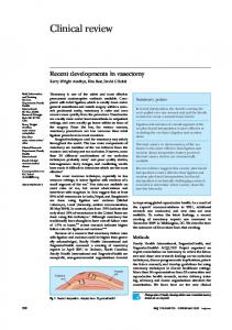
Observations in regression data essentially belong to four types: regular observations with internal x^ and well-fitting y^, vertical outliers with internal x; and non-fitting y;, good leverage points with outlying x^ and well-fitting y^ bad leverage points with outlying x; and non-fitting y;. Figure 1 shows these four types in simple regression. Regression diagnostics aim to detect observations of one or more of these types. Here we will consider three robust diagnostics: standardized residuals, the resistant diagnostic, and the diagnostic plot.
vertical outlier
good leverage point
regular data
• •
* bad leverage point
Figure 1: Simple regression data with points of all four types. lo Standardized residuals are defined as ri{θ)/s{θ) where s(θ) denotes a robust scale estimate based on the residuals. Here we will use 2 SLQS(Θ) = cfcιn|r(0)|fcn or sLTS(θ) = dh}n^Σir (θ)i:n. Standardized residuals help us to distinguish between well-fitting and non-fitting observations by comparing their absolute values to some yardstick, e.g. compare \n(θ)\/s(θ) to 2.5. We use the yardstick 2.5 since it would determine a (roughly) 99% tolerance interval for the e^ if they had a standard gaussian distribution. Since the standardized residuals approximate the e^, we will consider an observation as non-fitting if its standardized residual lies (far) outside this tolerance region.
Recent developments in PROGRESS
5 o
X regular observations
X
211
vertical outliers + bad leverage points
good leverage points
vertical outliers + bad leverage points
resistant diagnostic
Figure 2: Classification of observations by plotting the standardized residuals versus their resistant diagnostics. 2o The resistant diagnostic Non-regular observations have the property that they are 'far away' from some hyperplane in iR p + 1 (that is, further away than the majority of the observations). The vertical outliers and the bad leverage points are clearly far away from the ideal regression plane given by y = x^. But also a good leverage point lies far away, relative to some other hyperplane that goes through the center of the regular observations. To define the 'distance' of an observation (xi,ί/t) to a plane y = x*0 we can use its absolute standardized residual. If we now define \n(θ)\ li = sup i = sup or 7 SLTS{Θ) θ we expect outliers to have a large Ui. Since the Ui are difficult to compute exactly, we approximate them by taking the maximum over all θ that are computed inside the LQS/LTS algorithm. For each observation, this yields the value J!j^l (14) or tlί = m a x J ^ M . θ sLQS(θ) θ sLTs{θ) Therefore we only need to store one array (u\,... ,un) that has to be updated at each p-subset. Finally, we define the resistant diagnostic for each observation by standardizing the u^ yielding Ui
=
max
resistant diagnostic^ =
med
(15)
212
Peter J. Rousseeuw and Mia Hubert
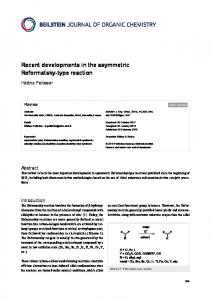
In the new version of PROGRESS the resistant diagnostic is available for both LQS and LTS, and it is based on the trial estimates θ after location adjustment. From (14) it is clear that non-regular observations will have a large U{ and consequently a large resistant diagnostic. Simulations have indicated that we may consider (15) as 'large' if it exceeds 2.5. Combining the standardized residuals with the resistant diagnostic leads to the diagram in Figure 2. However, a disadvantage of Figure 2 is that it cannot distinguish between vertical outliers and bad leverage points. 3o The diagnostic plot makes the complete classification into the four types. Since leverage points are outlying in the space of the regressors x^, one can distinguish them from vertical outliers by analyzing their x—components. For this we can run MINVOL OVLX — {x^; 1 < i < n). This program computes the Minimum Volume Ellipsoid (MVE) location estimate T{X) and scatter matrix C(X). The MVE is a highly robust estimator of location and scatter, introduced by Rousseeuw (1985). The corresponding robust distance of an observation to the center is then given by
Since the squares of these distances roughly have a chi-squared distribution when there are no outliers among the x^, we will classify an observation as a leverage point if its RDfa) exceeds the cutoff value Λ/X^O.975- ^ w e combine this information with the standardized LQS or LTS residual, we obtain the diagnostic plot of (Rousseeuw and van Zomeren, 1990) shown in Figure 3. cutoff
vertical outliers
bad leverage points
regular observations
good leverage points
vertical outliers
bad leverage points
1
robust distance RD(x,)
Figure 3: Diagnostic plot, obtained by plotting the standardized robust residuals versus the robust distances
Recent developments in PROGRESS
7
213
Software availability
The programs PROGRESS and MINVOL can be obtained from our website http://win-www.uia.ac.be/u/statis Questions or remarks about the implementation can be directed to
[email protected]. The LMS, LTS and MVE methods are also available in S-PLUS as the functions lmsreg, l t s r e g and cov.mve. Moreover, the functions LMS, LTS and MVE based on the recent versions of PROGRESS and MINVOL have been incorporated into SAS/IML (Version 6.12) in 1996. Their documentation can be obtained by writing to sasaxsOunx.sas.com.
Appendix: Proof of Theorem 1 We show that the proof of the breakdown value of the LMS (Rousseeuw, 1984, page 878) remains valid after making the necessary modifications. The proofs for LQS and LTS are very similar, so we will mainly consider the LQS estimator. First suppose h < [ n +P + 1 ]. We obtain the lower bound on ε* by replacing h — p + 1 — 1 = h — p observations of Z, yielding Z'. Define θ = Θ QS(Z) and ff — ΘLQS(Z'). The n-h+p>h original points (x»,y») then satisfy |ri(0)| = \yι — Xi0| < M = max^ K(0)| such that for the corrupted data set Z1, \ri(θf)\h:n < \ri(θ)\h:n < M. For p > 1 we refer to the geometrical construction of (Rousseeuw, 1984). In his notation, the set Z'\A contains at most n — {n — h + p — (p — I)) = h — 1 observations. If we assume ||0' - θ\\ > 2(||0|| + M / » , this implies L
\riψ')\h:n>M,
(16)
a contradiction. Therefore, ||0 7 || remains bounded. For p = 1 we set C = 2M/N = 2M/minz\xi\. Now suppose |0 - θ'\ > C. For all noncontaminated observations we have that \ri(θ) — ri(θ')\ = \yι — xiθ — yi — Xiff\ = \Xi\\θ - θ'\ > NC = 2M, from which we get 1^(0')! > \n{θ) ri(θf)\ - \ri(θ)\ > 2M - M = M. Again this implies (16) and thus a bounded θr. The upper bound on ε^ follows from the fact that we can put h — p + 1 bad observations on a hyperplane that contains p — 1 original points. Then (h - p + 1) + (p - 1) = h observations satisfy y[ = x^0r, and thus ff — ΘLQS(Z'). Making the hyperplane steeper will break down the estimator. For h > [ n + P + 1 ], we obtain the lower bound analogously to the previous case. Just observe that we now have n — in — h + I) + I — h original observations, and that Z' \ A has at most n - (h - (p - 1)) = n - h + p — I < h — 1 points. The remaining inequality ε* < (n — h + l)/ra can
214
Peter J. Rousseeuw and Mia Hubert
be proved as follows. Take some M > \\θ\\. Then we show that we can 1 always construct a corrupted sample Z with n — h + 1 bad observations, such that || M. Letting M go to infinity will then cause the LQS to break down. Define M j = max; ||x*||. Now we set all the n — h + 1 replaced observations equal to the point (x, y) = (x, 2MχM + K) for which ||x|| = M.χ and K > 0. These replaced observations satisfy M l < ||xi||||0|| < ||x||M = MXM < y and thus 1^(0)| - \y{ - x ^ | > \y\ - \κθ\ > MXM
+ K.
this yields \ri(θ)\hm
A s n - h + l > n - h
>
MxM + K. Since we can choose K arbitrarily large, the minimum of the objective function of LQS will not be reached for ||β|| < M. Consequently = II^ΊI IrLQsC^OII has to be larger than M, which ends the proof. Finally we note that using the same construction, the objective function of LTS satisfies 2
Σ(r (θ))i..n>(MxM
2
+ K)
yielding the same result.
References [1] Croux, C, Haesbroeck, G., and Rousseeuw, P.J. (1996). Location adjustment for the minimum volume ellipsoid estimator. Submitted for publication. [2] Donoho, D.L., and Huber, P.J. (1983). The notion of breakdown point. In A Festschrift for Eήch Lehmann, Eds. P. Bickel, K. Doksum, and J.L. Hodges. California: Wadsworth. [3] Rousseeuw, P.J. (1984). Least median of squares regression. J. Am. Statist Assoc. 79 871-880. [4] Rousseeuw, P.J. (1985). Multivariate estimation with high breakdown point. In Mathematical Statistics and Applications, Eds. W. Grossmann, G. Pflug, I. Vincze, and W. Wertz, Vol. B, pp. 283-297. Dordrecht: Reidel. [5] Rousseeuw, P.J., and Leroy, A.M. (1987). Robust Regression and Outlier Detection.New York: Wiley. [6] Rousseeuw, P.J., and van Zomeren, B.C. (1990). Unmasking multivariate outliers and leverage points. J. Am. Statist Assoc. 85 633-639. [7] Steele, J.M., and Steiger, W.L. (1986). Algorithms and complexity for least median of squares regression. Discrete Applied Mathematics 14 93-100.