Recent developments in the multi-scale-finite-volume procedure Giuseppe Bonfigli1 and Patrick Jenny1 ETH-Zurich, CH-5092 Zurich, Switzerland,
[email protected]
Abstract. The multi-scale-finite-volume (MSFV) procedure for the approximate solution of elliptic problems with varying coefficients has been recently modified by introducing an iterative loop to achieve any desired level of accuracy (iterative MSFV, IMSFV). We further develop the iterative concept considering a Galerkin approach to define the coarse-scale problem, which is one of the key elements of the MSFV and IMSFVmethods. The new Galerkin based method is still a multi-scale approach, in the sense that upscaling to the coarse-scale problem is achieved by means of numerically computed basis functions resulting from localized problems. However, it does not enforce strict conservativity at the coarsescale level, and consequently no conservative velocity field can be defined as in the IMSFV-procedure until convergence to the exact solution is achieved. Numerical results are provided to evaluate the performance of the modified procedure.
1
Introduction
The multi-scale-finite-volume (MSFV) procedure by Jenny et al. [1] is a method for the approximate solution of discrete problems resulting from the elliptic partial differential equation ∇ · λ∇φ = q,
x ∈ Ω, λ > 0,
(1)
when the operator on the left-hand side is discretized on a Cartesian grid with standard five-point stencils. The coefficient λ can be an arbitrary function of the spatial coordinate x. Successive developments of the MSFV-approach have been proposed by Lunati and Jenny [2], Hajibeygi et al. [3] and Bonfigli and Jenny [4]. The iterative version, i.e. the IMSFV-method, has been introduced in [3] and modified in [4] to improve its efficiency in cases in which the coefficient λ varies over several orders of magnitude within the integration domain. The IMSFV-method as presented in [4] foresees two steps for the computation of the approximate solution at each level of the iterative loop: the fine-scale step or fine-scale relaxation and the coarse-scale step. The fine-scale step requires the solution of several localized problems on subdomains of the original grid with approximated boundary conditions. This allows to capture the finescale features in the spatial distributions of the coefficient λ and of the source
2
term q. However, due to the local character of the considered problems, the interdependence of any two points in the integration domain, as implied by the elliptic character of equation (1) (global coupling), can not be accounted for at this stage. Analogies are found here with domain decomposition approaches, in particular if Dirichlet boundary conditions for the localized problems are extracted in the IMSFV-method from the solution at the previous iteration [4]. If the subdomains are reduced to a grid line or to a single grid point, standard line or Gauss-Seidel-relaxation is recovered. The coarse-scale step provides the global coupling missing in the fine-scale step. An upscaled problem with a strongly reduced number of degrees of freedom (coarse-scale problem) is defined by requiring the integral fulfillment of the conservation law (1) for a set of coarse control volumes. This provides an approximate solution on a coarse grid spanning the whole integration domain, which is then prolonged to the fine grid as in a two-level multi-grid approach [3, 4]. The main novelty of the IMSFV-procedure considered as an elliptic solver is represented by the strategy used for restriction and prolongation, i.e. to define the coarse-scale problem and to interpolate its solution back to the fine grid. Both steps are achieved by means of the basis functions computed by solving numerically localized problems at the fine-scale level, such that the fine-scale features of the coefficient λ are approximatively accounted for. Even if the efficiency of the MSFV and IMSFV-methods have been demonstrated for several applications, some aspects still deserve further investigation. In particular: – The stability of the iterative procedure for critical λ-distributions has been progressively improved [3, 4], but problems where the procedure diverges may still be found. – For large cases, the size of the coarse-scale problem may become significant, thus making a direct solution impracticable. The introduction of a further upscaling step, in analogy with multi-grid methods, would be an attractive alternative. The critical aspect with respect to the first point is clearly the quality of the coarse-scale operator. At the same time the structure of the coarse-scale problem also matters for the development of a multi-level procedure. The present investigation considers an alternative definition of the coarsescale problem based on a Galerkin approach, which, as usual for Galerkin methods, leads to a symmetric positive-definite or semi-definite system matrix. This is clearly a desirable feature in view of the targeted development of a multi level procedure. Due to its analogy with a Galerkin-based finite-element approach we call the new procedure iterative-multi-scale-finite-element method (IMSFE). As a preliminary step towards a multi-level method, we compare the performance of the IMSFE-procedure with that of the original IMSFV procedure, when the coarse-scale problem is solved directly. The base-line formulation of the IMSFVprocedure is the one presented in [4]. We point out that Galerkin, also iterative, approaches have been already used in the context of multi-scale methods for elliptic problems, beginning with the
3
seminal work by Hou and Wu [5] (see also [6]). The novelty of our contribution is rather their application in the context of the iterative strategy from the IMSFVmethod, i.e. considering basis functions as defined in the IMSFV-procedure and including line or Gauss-Seidel relaxation to converge at the fine-scale level.
2
The IMSFV-procedure
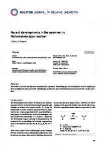
An extensive discussion of the IMSFV-procedure can be found in [3, 4]. Here we only present the basics. The different grids considered for the formulation of the IMSFV-procedure are sketched in figure 1. The so-called coarse and dual grids, are staggered with respect to each other and their cells (coarse and dual cells) are defined as rectangular blocks of cells from the original grid (fine grid). Neighbouring dual cells share one layer of fine-grid cells (right bottom figure). Let P be the index set for an indexing of the fine-grid cells. The unknowns of the fine-scale problem are the values φj , j ∈ P, of the discrete solution φ at centroids xj of the fine cells. The unknowns of the coarse-scale problem are the values φj , j ∈ P¯ ⊂ P at fine-grid nodes corresponding to the corners of dual cells (coarse-grid nodes, crosses in figure 1).
¯j Ω ˜j Ω
¯ j , solid lines) and dual grid (cells Ω ˜j , dashed lines) with enlargeFig. 1. Coarse (cells Ω ment of the corner region of coarse (top) and dual cells (bottom). Thin lines mark the boundaries of fine-grid cells, thick lines the boundaries of coarse and dual cells.
Given the approximate solution φ[n] the improved solution φ[n+1] at the next iteration step is given by φ[n+1] = S ns (φ[n] + δφ),
(2)
where S in the fine-scale relaxation operator (we only consider line and GaussSeidel relaxation), which is applied ns times after adding the correction δφ from the coarse-scale step to the old solution. In turn, the correction δφ is defined as the linear superposition X δφj Φj (3) δφ = ¯ j∈P
4
¯ provided by of the basis functions Φj , scaled with the node-values δφj , j ∈ P, the solution of the coarse-scale problem. Once the basis functions are assigned, the coarse-scale problem, i.e. a linear ¯ is obtained by requiring the system for the coarse-scale unknowns δφj , j ∈ P, conservation law represented by equation (1) to be fulfilled by (φ[n] + δφ) for all ¯j . By considering the divergence theorem and the definition (3) of coarse cells Ω δφ, one obtains the following equivalent sets of equations: Z Z ¯ qdV, j ∈ P, (4a) ∇ · λ∇(φ[n] + δφ)dV = ¯j Ω
¯j Ω
X
¯ k∈P
δφk
Z
¯j ∂Ω
λ∇Φk · ndS = −
Z
¯j ∂Ω
λ∇φ[n] · ndS +
Z
¯j Ω
qdV,
¯ j ∈ P,
(4b)
of which the latter is usually implemented in the IMSFV-procedure. Of course, the discrete version of the equations is considered in the numerical procedure, where the integration and differentiation operators are replaced by the corresponding discrete operators. The equivalence of equations (4a) and (4b) is preserved also in the discrete case, since the divergence theorem holds exactly for the considered finite-volume discretization. In conclusion, we detail the definition of the basis functions Φj , each of which is non-zero only within the dual cells intersecting the corresponding coarse cell ¯j . Fix j ∈ P¯ so that no face of Ω ¯j lies on the domain boundary ∂Ω and let Ω ˜k Ω ˜k ∩ Ω ¯j 6= ∅. Let furthermore C ⊂ P¯ be the set of indices of be a dual cell so that Ω ˜k . The restriction of Φj to the coarse-grid nodes xl corresponding to corners of Ω ˜ Ωk is then determined by the following localized elliptic problem with so-called reduced boundary conditions: ˆ ∇ · λ∇Φ j = 0,
˜k , x∈Ω
(5a)
Φj = 0, Φj = 1, ˆ t Φj = 0, ∇t · λ∇
x = x l , l ∈ C \ {j}, x = xj , ˜k . x ∈ ∂Ω
(5b) (5c) (5d)
Thereby, the tangential nabla operator ∇t = ∇ − n(n · ∇) is defined at boundary ˜k analogously to ∇, but ignores derivatives in direction normal points x ∈ ∂ Ω ˆ = max{λ, Λ}, ˆ Λˆ > 0, follows from to the boundary. The modified coefficient λ λ after removing very low values to avoid bad conditioning of the coarse-scale problem [4]. For numerical implementation, the discretized version of equation ˜k , leading (5d) is imposed in place of (5a) for cells adjacent to the boundary ∂ Ω ˜k , with Dirichlet-like boundary conditions to 1-d problems along the edges of ∂ Ω ˜k lie on the domain given by (5b) and (5c). Finally, if one or more edges of Ω boundary, the homogeneous counterpart of the boundary condition prescribed for the solution φ are imposed there in place of equation (5d). The consistency of the definition of Φj at fine-grid nodes shared by more than one dual cell and their suitability to define the coarse system are discussed in [3, 4].
5
3
The Galerkin approach
The coarse-scale problem in its form (4a) can be interpreted as a weak formulation of the elliptic equation (1) considering the test functions ( ¯j 1, x ∈ Ω ¯ χΩ¯j = , j ∈ P. (6) ¯ 0, x ∈ / Ωj The obvious alternative considered in this work is represented by the Galerkin approach, in which the basis functions themselves are considered as test functions [5, 6]. The following equivalent coarse-scale problems are derived: Z Z ¯ Ψj qdV, j ∈ P, (7a) Φj [∇ · λ∇(φ[n] + δφ)]dV = Ω Ω Z Z X ¯ δφk Φj ∇ · λ∇Φk dV = Φj (−∇ · λ∇φ[n] + q)dV, j ∈ P, (7b) Ω
¯ k∈P
X
¯ k∈P
δφk
Z
Ω
∇Φj · λ∇Φk dV =
Ω
Z
Φj (−∇ · λ∇φ[n] + q)dV,
¯ j ∈ P.
(7c)
Ω
Summations needed to evaluate the volume integrals in the discrete case, may be limited to cells in the support of Φj and their immediate neighbours. The formulation (7c) of the coarse-scale problem shows that the system matrix is symmetric and positive definite, except for problems with Neumann conditions on the whole boundary, for which it is positive semi-definite, with one single eigenvalue equal to zero. Constant φ-distributions are in this case the only non-trivial elements of the matrix null-space [4]. Correspondingly, the system is uniquely solvable if the boundary conditions are not only Neumann. In the opposite case, the solution exists, and is determined up to an additive constant, only if the usual compatibility constraint between Neumann boundary conditions and source term is fulfilled. The effects of the Galerkin approach on the performance of the complete iterative procedure are not as evident. Numerical experiments investigating this aspect for a challenging distribution of the coefficient λ are presented in the following section. We point out that the original IMSFV procedure provides at any convergence level of the iterative procedure an approximation g˜ for the gradient ∇φ, so that ∇ · g˜ = q (conservative vector field). This is not true for the Galerkin-based IMSFE-procedure, for which only the fully converged solution is conservative.
4
Numerical tests
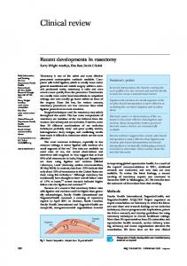
We consider the elliptic problem of the form (1), which has to be solved in the simulation of incompressible flows in porous media. The coefficient λ corresponds to a 2-d slice of the permeability field for the SPE-10-bottom-layer test case for reservoir simulations [7]. The fine grid contains 220 × 60 cells, equally divided
6
into 22 × 6 coarse cells. Concentrated sinks and sources of equal intensity and opposite sign are set at two opposite corners of the integration domain. The distribution for λ and the fine-scale solution are displayed in figure 2. 60 y
Log(λ) 44 3 22 1 00 -1 -2 -2
40 20 00
50
100
150
x 200
p 0.01 0.00 -0.01 0y
50 x
0
100 150 25
50
200
Fig. 2. Permeability distribution and solution. Lines in left figure correspond to the boundaries of the coarse cells, circles to the coarse-grid nodes.
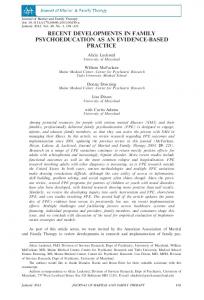
Convergence rates Γ for the IMSFV and IMSFE-procedures are presented in figure 3 for different values of the lower bound Λˆ (see equation (5)) and for different stretching factors α = ∆x/∆y of the fine-grid cells. The coefficient λ is assumed to be constant within fine cells for the discrete formulation of the problem, and the value associated to each cell is not modified when varying α. Result are presented for computations in which fine-scale relaxation is obtained either by line (ns = 10) or Gauss-Seidel relaxation (ns = 20, each line-relaxation step includes two steps comparable to a Gauss-Seidel step, one for each spatial direction). The convergence rate Γ is defined as Γ = 1/N , where N is the average number of iterations needed to reduce the error ǫ = ||φ[n] − φ||∞ by one order of magnitude. We evaluate Γ considering iterations for which 10−5 ≤ ǫ ≤ 10−3 . If α ≫ 1, the connectivity between fine cells sharing edges normal to the yaxis is much larger than for cells sharing faces normal to the x-axis (anisotropic problems). This is known to be a critical situation, and similar problems could be handled successfully by IMSFV only after including line-relaxation in the finescale step [3]. The robustness of the iterative procedure in this respect was enˆ for the computation of basis hanced by introducing the clipped coefficient field λ functions [4]. Figure 3 shows that a further significant improvement may be accomplished by considering the Galerkin-based coarse system. On the other hand, the stability envelope of the original procedure can be enlarged only marginally by increasing the number ns of relaxation steps. Convergence rates for stable computations depend only moderately on the strategy considered to define the coarse-scale problem. However, the improved ˆ which stability of the Galerkin approach simplifies the choice of lower bound Λ, in the standard procedure is not easy, since, for a given α, the optimal value of Λˆ is often close to the limit of the stability region. When using the Galerkinbased approach, a reasonable choice for moderate α would be Λˆ = 0 (no lower
7 3
3
α
α
2
2
1
1
0
-6
-4
-2
ˆ Λ/||λ|| ∞
0
0
3
3
α
α
2
2
1
1
0
-6
-4
-2
0 ˆ Λ/||λ|| ∞
0
-6
-4
-2
ˆ Λ/||λ|| ∞
0
-6
-4
-2
0 ˆ Λ/||λ|| ∞
log10 (Γ )
Fig. 3. Convergence rates for the IMSFE (left colum) and the IMSFV-procedures (right column) considering line relaxation (ns = 10, top row) or Gauss-Seidel relaxation (ns = 20, bottom row) for fine-scale relaxation. Blanked values indicate divergence of the iterative procedure.
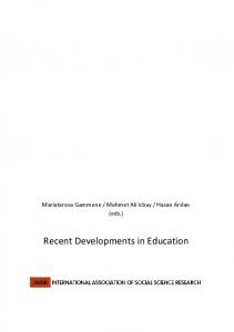
bound). For very large stretching factors α, the performance is not satisfactory, neither for the IMSFV, nor for the IMSFE-procedure. The highest convergence ˆ rates are obtained for Λ/||λ|| ∞ = 1, i.e. when the basis functions are computed for a homogeneous λ-distribution. In this case the IMSFV-approach performs slightly better. If Λˆ is decreased, the IMSFV-procedure becomes unstable, while convergence rates for the Galerkin based approach decrease to the level provided by the fine-scale relaxation step. Better results for anisotropic problems, could be achieved by modifying the number of fine cells per coarse cell so to keep the aspect ratio of the latter close to one. Convergence rates are consistently higher if line relaxation is used in place of Gauss-Seidel relaxation. The dependence of Γ on the number ns of relaxation steps is investigated in −2 ˆ figure 4 for Λ/||λ|| . Convergence rates are found in all cases to grow ∞ = 10 proportionally to ns . Since fine-scale relaxation represents a relevant portion of the computational costs, no determinant gain of performance can be attained by increasing ns .
5
Conclusions
A Galerkin formulation has been proposed for the coarse-scale problem of the IMSFV-procedure, leading to a symmetric positive-definite or semi-definite matrix. This is equivalent to using a finite-element approach at the coarse level [5, 6]. Numerical testing has been carried out considering one challenging spatial
8 10
0
0
10
Γ
ns ns ns ns ns
Γ -1
10
-1
10
-2
10
=5 = 10 = 15 = 20 = 300
-2
10
-3
10 10
10
ns ns ns ns ns
-3
=5 = 10 = 15 = 20 = 300
-4
10
-4
10
-5
0
10
1
10
2
3
α
10
10
0
10
1
10
2
10
3
α
10
Fig. 4. Convergence rates for the IMSFE (lines) and the IMSFV-procedures (lines with symbols) as functions of the number ns of fine scale relaxation steps and of the grid −2 ˆ stretching α with Λ/||λ|| . Fine-scale relaxation is achieved either by means ∞ = 10 of line-relaxation (left) of Gauss-Seidel relaxation (right).
distribution of the coefficient in the elliptic problem (permeability field according to the terminology used for incompressible flows in porous media). If the coarse system is solved directly as usual in IMSFV, the resulting IMSFE-procedure is significantly more stable than the original one. For cases where both procedure converge, differences in their convergence rates are moderate. These results seem to indicate that the Galerkin-based approach, due to the favourable features of the coarse-scale-system matrix, could be a good starting point for the generalization of IMSFV as a multi-level procedure. Further tests considering different permeability distributions are needed to allow conclusive statements.
References 1. Jenny, P., Lee, S.H., Tchelepi, H.A.: Multi-scale finite-volume method for elliptic problems in subsurface flow simulation. J. Comp. Phys. 187 (2003) 47–67 2. Lunati, I., Jenny, P.: Multiscale finite-volume method for density-driven flow in porous media. Comput. Geosci. 12 (2008) 337–350 3. Hajibeygi, H., Bonfigli, G., Hesse, M.A., Jenny, P.: Iterative multiscale finite-volume method. J. Comp. Phys. 277 (2008) 8604–8621 4. Bonfigli, G., Jenny, P.: An efficient multi-scale poisson solver for the incompressible navier-stokes equations with immersed boundaries. J. Comp. Phys. (2009) accepted. 5. Hou, T.Y., Wu, X.H.: A multiscale finite element method for elliptic problems in composite materials and porous media. J. Comp. Phys. 134 (1997) 169–189 6. Efendiev, Y., Hou, T.Y.: Multiscale Finite Element Methods: Theory and Application. 1st edn. Springer (2009) 7. Christie, M.A., Blunt, M.J.: 10th SPE comparative solution project: a comparison of upscaling techniques. In: SPE 66599. (February 2001)