RECENT DEVELOPMENTS ON 3D MODELING OF RANDOM ROUGH SURFACES M. Y. Xia(1), C. H. Chan(2), L. Tsang(3), M. Saillard (4), and G. Soriano(5) (1)
Wireless Communications Research Center, City University of Hong Kong 83 Tat Chee Ave, Kowloon, Hong Kong, China,
[email protected] (2) As (1) above, but E-mail:
[email protected] (3) As (1) above, but E-mail:
[email protected] (4) Institut Fresnel, UMR CNRS 6133, Faculté Saint Jérôme, case 162 13397 Marseille Cedex 20, France,
[email protected] (5) As (4) above, but E-mail:
[email protected]
ABSTRACT Recent advancements on 3D modeling of random rough surface are reported in this paper. A multilevel sparse-matrix canonical grid method is adopted to solve the matrix equation resulted from a single integral equation formulation in conjunction with the vector triangular basis functions. Both the beam decomposition technique for analyzing large surfaces and the impedance approximation method suitable for highly conductive media are also incorporated into the solution method. Essentials of the algorithms are explained and numerical results are presented for wind-driven ocean surfaces. INTRODUCTION Random rough surface scattering has been a topic of continued study for many years and it has drawn an increasing attention in the past decade [1]-[2] because of its broad applications. These applications include microwave remote sensing of wind field over ocean, microwave remote sensing of soil moisture, backscattering enhancement in on-board radar collision avoidance systems, and optical nondestructive evaluation of material and metallic finishes. Common to these applications is the need of a finer surface discretization and/or larger surfaces, which translate to solving a larger system of equations than what has been previously attempted. In this paper, we will present recent advancements made individually by the two research teams from Hong Kong and France and the integration of their methods for solving larger and rougher surfaces. For three-dimensional simulations of dielectric surface of thousands of square wavelengths, a MoM equation up to several millions of unknowns has to be solved. It is crucial for an efficient algorithm to achieve a considerable reduction both in computer memory storage requirement and CPU time. To this end, the Hong Kong team has developed the sparse-matrix canonical-grid (SMCG) method [3] that entails the use of fast Fourier transforms (FFTs) for speeding up the computation while simultaneously reducing the computer memory requirement upon a Taylor series expansion of the Green’s functions over a flat surface. This scheme has recently been extended for rougher surfaces by expanding the Green’s function over several horizontal planes transverse to the surface [4]. Recognizing that the Green’s functions in the lossy medium with high permittivity decay rapidly, the two-grid SMCG method [5] is developed so that the accuracy of a fine discretization in the dielectric region can be achieved while the efficiency of using a coarse grid in the air region can be maintained. We further reduce the number of unknowns by half via the adoption of a single integral equation formulation [6]. Another approach to reduce the memory storage requirement is to decompose the incident beam into smaller ones so that the original large problem can be transformed to solving a set of substantially reduced smaller problems. The French team adopted this beam synthesis approach successfully in conjunction with the earlier version of the SMCG method [7]. Their numerical results agree well with experiment for conducting surfaces. By using the impedance boundary condition that replaces the integral operator linking the electric and magnetic surface currents by a local relationship, the number of unknowns is also reduced by a factor of two. This approach has lead to very accurate results in the case of metallic surfaces in optics, where it has been compared with experimental results. The goal of this paper is to combine the merits of these techniques to address the rough surface scattering problem. In particular, since a great challenge in passive and active remote sensing is to develop accurate models for bistatic scattering from sea surfaces, we will present results on the validation of the impedance approximation approach by comparing it with the single integral equation formulation for wind-driven sea surfaces [8]. In the microwave frequency range, both the real and imaginary parts of the permittivity of seawater are very high. All of these algorithms are implemented on a low-cost PC-based parallel computing platform, and the largest number of unknowns solved so far is over six million with
all the coherent interactions included. Much larger surfaces can be tackled if the beam synthesis approach is activated, although some more CPU time will be consumed because overlapping of the adjacent beams are required. OUTLINE OF THE ALGPRITHM The governing equation adopted is the single magnetic field integral equation formulation [9]. Using the Method of Moments with the Rao-Wilton-Glisson (RWG) basis function, a linear equation set is arrived:
(M s + M w ) ⋅ x = b
(1) where x represents the surface effective current to be resolved, which contains N unknowns associated with the N interior edges of the triangulated patches, and b corresponds to the excitation due to the incident field. Matrix M s denotes the near-strong interactions within a distance r between a source point and an observation point, and M w the far-weak interactions beyond r. The elements of the strong parts are calculated by exact numerical integration and stored in computer memory. However, the elements of the weak parts are not calculated nor stored in conventional ways. By expending the Green’s function and its gradient as Taylor series about a grid coordinate system, it can be shown that the weak elements have the following form: K
M w (n, n' ) = ∑ f k (n)U k (n − n' )g k (n' )
(2)
k =0
where K truncates the terms of the Taylor series expansion; f k is a column vector associated with the N observation points; and g k associated with the N source locations. The matrix U k has the Toeplitz structure that may be stored as a vector with 2 N − 1 data. For a multi-dimensional problem, the grid index in (2) should be understood as
n = (n x , n y , n z ) and n − n' = (n x − n' x ,L) . The reduction of memory storage requirement is achieved as follows. The storage of the original full matrix is O( N 2 ) . The storage of M s is proportional to O(N ) because at each observation point only a few near source elements within the given distance r are taken into account. The storage of U k is O(2 N ) , so is f k and g k with N zeros padded to each of them to make use of the FFT. Thus, the total storage of ( M s + M w ) is scaled down to O(αN ) where α is a constant typically less than a few tens. The memory storage saving is huge if N is as large as several millions. The equation (1) is solved using the conjugate gradient method (CGM), by which no matrix inversion but matrix-vector multiplication is involved. The multiplication of the strong part with a column vector takes little time, as the matrix is very sparse. Thanks to the approximation (2), the multiplication of the weak part with a column vector can be accelerated tremendously using the FFT technique, i.e., K
M w x = ∑ f k ⋅ FFT −1{FFT[U k ] ⋅ FFT[g k ⋅ x]}
(3)
k =0
Direct computation of the left-hand side is O( N 2 ) . However, because the computing complexity of the three FFT is 3 × (2 N log 2 N ) and that of the three products is 3 × (2 N ) , the total computing burden of the right-hand side is only O( βN ) where β = ( K + 1)(6 log 2 N + 6) which may be seen as a constant as log 2 N varies very slowly with N . Thus, the saving of CPU time for an iterative solution is appreciable as β is typically several hundreds while N on the order of millions. The above algorithm is extremely robust for a range of surface sizes and roughness. Using a cluster of 32 CPU each with 256 MB RAM, it can handle over six millions surface unknowns representing the equivalent electric and magnetic currents for a dielectric surface or the induced currents for a perfect conducing surface. If the surface size is so large that the memory saving strategy fails, a beam decomposition technique may be activated. This is particularly suited to some parallel computers that have many processors but a stringent amount of RAM. By decomposing the incident wave as many narrower beams, the total scattering fields can be synthesized coherently from the partial scattering fields of the individual beams in merit of the linearity of the Maxwell equations, i.e.,
r r E Bi , s = ∑ Wmn Ebi ,,smn
(4)
m,n
where the superscript indicates the incident field or scattering field; the subscript B and b indicate the big beam or small beams; and Wmn are weighting factors. A typical decomposition is to choose the full width of a narrow beam to be half that of the large beam and to move the narrow beam at a step of one-fourth the full width of the narrow beam, thus to yield a total of 25 smaller beams. The original problem is translated to solve 25 small problems and coherently adding the results. In general, for a direct application of the MoM, the currents must be sampled sufficiently, typically 10 points per linear wavelength in the denser medium or the skin-depth scaled for a conductive medium. This will produce a prohibitively large number of unknowns for a high lossy medium such as seawater at microwave frequencies, though the simulated size is not very large. In this case, the impedance approximation method may be applied, which allows the sampling to take at a much coarser discretization, usually 8 points per linear wavelength in free space. The accuracy has been confirmed to be satisfactory for seawater at L-band by comparing the results with those obtained at much denser sampling of 32 points per linear wavelength. Parallel implementation of the above algorithm is as follows. A random rough surface satisfying the given statistical property is generated by one of the computers and the profile data is broadcast to others. Each processor seeks a part of the strong matrix and stores the elements in their own memory using a sparse matrix storage strategy. When the strong matrix is multiplied with a column vector, each processor yields a local vector and the resultant vector is then assembled. For the multiplication of the weak matrix with a vector by the FFT algorithm described above, we have used the MPI version of the FFTW software [10], by which each processor only stores a portion of the transform vector. Thus, the storage requirement for each processor is a portion of the strong matrix and a portion of a vector involved in the FFT calculations. Essential immediate storage is carefully distributed to individual computers subject to less communications for later use. Once the equation set is solved, i.e., the effective surface current is found, the endpoint of the numerical analysis is to calculate the scattering fields and bistatic scattering coefficients. Each processor computes the scattering fields from a portion of the surface, then the total scattering fields is retrieved by adding the partial fields coherently and the scattering coefficients is to be calculated. If the beam decomposition method is activated, the above procedure applies to each sub-surface, and the resultant scattering fields is retrieved through adding the weighting fields from each portion. Another parallelism scheme is that each processor independently handles one beam at a time so that little communication is needed until the final synthesis. In this case, the memory of one processor is not shared with others and thus the subbeams should be narrow enough so that one processor can handle one beam its own. Another disadvantage of this design is difficult to evenly load the processors, say there are 32 CPU but 36 beams to handle.
NUMERICAL EXAMPLES Our computing platform is a cluster of 32 PIII 670 MHz CPUs, each with 256 MB RAM. An iterative solution is admitted when the error norm is less than 1%, i.e.,
||Ri||/||b|| < 1% where Ri = b − ( M s + M w ) x i . The permittivity of the
seawater is taken to be 74+i61 at 1.5 GHz. A fitted power-law spectrum function at wind speed 10 m/s over the sea surface is used:
W (k , φ ) =
5.25 × 10 −3 (1 + 13 cos 2φ ) 4 2π k
(5)
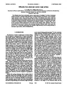
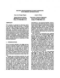
The interval of the wave number is confined to 1 ≤ k < 120 , so that the rough ocean surface driven by the wind field has a root-mean-square (rms) height of 0.25 wavelength and a rms slope of 0.112 wavelength at 1.5 GHz. The surface size taken for numerical experiments are 32 by 32 square-wavelengths. Numerical results are presented as bistatic scattering coefficients in the plane of incidence illuminated by a Gaussian tapered vector wave [11] at an incident angle of − 20 o . Fig.1 shows a comparison of the results using the localized impedance approximation method at 1/8 wavelength sampling with the exact results using the single integral equation formulation at 1/16 wavelength sampling. It shows that the approximate method can well characterize the feature of scattering fields at good precision for the permittivity of seawater being examined. Fig.2 shows the convergence of Monte-Carlo simulations with variable realizations for a TE wave incidence using the single integral equation formulation. The diamond data are computed for 37 by 37 square-wavelength surfaces. This explains why the peak of the scattering coefficients is slightly higher than that of the 32 by 32 surfaces while at other scattering angles they are lower. More numerical results will be provided at the conference.
10 exact, hh exact, vh appr., hh appr., vh
0 -10
scattering coefficients (dB)
scattering coefficients (dB)
10
-20 -30 -40 -50 -60
0 -10 -20 -30 -40 -50
-80
-60
-40
-20
0
20
40
60
scattering angle
Fig. 1 Comparison of using the localized approximation with exact results.
80
one realization 10 realizations 50 realizations
-80
-60
-40
-20
0
20
40
60
80
scattering angle
Fig. 2 Convergence of the scattering coefficients with increasing realizations.
REFERENCES [1] M. Saillard and A. Sentenac, “Rigorous solutions for electromagnetic scattering from rough surfaces,” Waves in Random Media, Vol.11, pp.R103-R137, 2001. [2] K.F. Warnick and W.C. Chew, “Numerical simulation methods for rough surface scattering,” Waves in Random Media, Vol.11, pp.R1-R30, 2001. [3] K. Pak, L. Tsang and J.T. Johnson, “Numerical simulations and backscattering enhancement of electromagnetic waves from two-dimensional dielectric random rough surface with the sparse-matrix canonical-grid method,” J. Opt. Soc. Am. A, vol.14, pp.1515-1529, 1997. [4] Q. Li, L. Tsang, J.C. Shi and C.H. Chan, “Application of physics-based two-grid method and sparse matrix canonical grid method for simulation of emissivities of soils with rough surfaces at microwave frequencies,” IEEE Trans. Geoscience and Remote Sensing, vol.38, pp.1635-1643, 2000. [5] S.Q. Li, C.H. Chan, M.Y. Xia, B. Zhang and L. Tsang, “Multilevel expansion of the sparse-matrix canonical-grid method for two-dimensional random rough surfaces,” IEEE Trans. Antennas & Propagat., vol.49, pp.1579-1589, 2001. [6] M.Y. Xia, C.H. Chan, S. Q. Li, B. Zhang and L. Tsang, “An efficient algorithm for electromagnetic scattering from rough surfaces using a single integral equation and multilevel sparse-matrix canonical-grid method,” IEEE Trans. Antennas & Propagat., accepted for publication subject to minor revisions. [7] G. Soriano and M. Saillard, “Scattering of electromagnetic waves from two-dimensional rough surfaces with an impedance approximation,” J. Opt. Soc. Am. A, vol.18, pp.124-133, January 2001. [8] T. Elfouhaily, B. Chapron and K. Katsaros, “A unified directional spectrum for long and short wind-driven waves,” J. Geophysical Research, vol.102, no.C7, pp.15781-15796, July 1997. [9] M. S. Yeung, “Single integral equation for electromagnetic scattering by three-dimensional homogeneous dielectric objects,” IEEE Trans. Antennas Propagat., vol.47, pp.1615-1622, 1999. [10] M. Frigo and S.G. Johnson, “The fastest Fourier transform in the west,” Tech. Rep., MIT-LCS-TR-728, 1997. (also see http://www.fftw.org). [11] H. Braunisch, Y. Zhang, C.O. Ao, S.E. Shih, Y.C. Eric Yang, K.H. Ding, J.A. Kong, and L. Tsang, “Tapered wave with dominant polarization state for all angles of incidence,” IEEE Trans. Antennas Propagat., vol.48, pp.1086-1096, July 2000.