Receptor Modeling of Ambient Particulate Matter Data Using Positive ...

TECHNICAL PAPER

ISSN 1047-3289 J. Air & Waste Manage. Assoc. 57:146 –154 Copyright 2007 Air & Waste Management Association

Receptor Modeling of Ambient Particulate Matter Data Using Positive Matrix Factorization: Review of Existing Methods Adam Reff and Shelly I. Eberly National Exposure Research Laboratory, U.S. Environmental Protection Agency, Research Triangle Park, NC Prakash V. Bhave Atmospheric Sciences Modeling Division, Air Resources Laboratory, National Oceanic and Atmospheric Administration, Research Triangle Park, NC

ABSTRACT Methods for apportioning sources of ambient particulate matter (PM) using the positive matrix factorization (PMF) algorithm are reviewed. Numerous procedural decisions must be made and algorithmic parameters selected when analyzing PM data with PMF. However, few publications document enough of these details for readers to evaluate, reproduce, or compare results between different studies. For example, few studies document why some species were used and others not used in the modeling, how the number of factors was selected, or how much uncertainty exists in the solutions. More thorough documentation will aid the development of standard protocols for analyzing PM data with PMF and will reveal more clearly where research is needed to help future analysts select from the various possible procedures and parameters available in PMF. For example, research likely is needed to determine optimal approaches for handling data below detection limits, ways to apportion PM mass among sources identified by PMF, and ways to estimate uncertainties in the solution. The review closes with recommendations for documenting the methodological details of future PMF analyses. INTRODUCTION Positive matrix factorization (PMF) is a recent development in the class of data analysis techniques called factor analysis,1 in which the fundamental problem is to resolve the identities and contributions of components in an

IMPLICATIONS Numerous recent studies have performed source apportionment of ambient PM using the PMF receptor model. After summarizing the methods of previously published papers, the authors recommend that future publications fully document the procedures used to prepare PM data, apply PMF, and interpret the results. This will ensure that future analyses of PM data with PMF are based on clear and precise methods, which will aid in both future research of atmospheric PM and in using PMF in the development of air quality management strategies.

146 Journal of the Air & Waste Management Association

unknown mixture.2 PMF has been used extensively for source apportionment of ambient particulate matter (PM), where the goal is to resolve the mixture of sources that contributes to PM samples. PMF is especially applicable to working with environmental data because it: (1) incorporates the variable uncertainties often associated with measurements of environmental samples and (2) forces all of the values in the solution profiles and contributions to be nonnegative, which is more realistic than solutions from previously used methods like principal components analysis. Modern-day sampling networks, such as the Speciation Trends Network (STN),3 the Interagency Monitoring of Protected Visual Environment (IMPROVE) Network,4 and the Southeastern Aerosol Research and Characterization (SEARCH) Study Network,5 provide time-resolved speciated ambient aerosol data that include trace and crustal elements, ions, organic (OC) and elemental carbon (EC) fractions, and PM concentrations. PMF has been used to identify and apportion sources of airborne PM by analyzing these species (or a subset) measured at numerous locations around the United States, including urban locations, such as Phoenix, AZ6; Washington, DC7; Houston, TX8; Narragansett, RI9; New York, NY10,11; Seattle, WA12; Atlanta, GA13–16; and Baltimore, MD17; and at rural and remote locations, such as Vermont18,19; Alaska20; Spokane, WA21; Potsdam and Stockton, NY22; Brigantine, NJ23,24; and San Gorgonio, CA.25 Similar methods have been applied to locations outside the United States, such as Bangladesh26; Thailand27; the Arctic region28; Chile29; Vietnam30; Ireland31; Hong Kong32–34; Toronto, Canada35,36; Beijing37,38; Spain39; New Zealand40; the U.K.41; and Finland.42 Profiles and contributions of PM from primary sources, such as motor vehicles, residential and industrial fuel combustion, biomass burning, soil dust, and sea salt are typically identified by PMF analyses in these studies. Secondary sources, such as atmospheric oxidation of sulfate and nitrate and heterogeneous gas-to-particle conversion reactions on soil dust surfaces, have also been identified with PMF.43 Despite the extensive use of PMF, there exists considerable variation in the procedures followed and decisions made to apportion sources of ambient PM using PMF. This paper summarizes the different procedures and Volume 57 February 2007

Reff, Eberly, and Bhave decisions available in published literature regarding the modeling of time-resolved, speciated ambient PM data using PMF. The modeling procedures may be divided into three broad steps: (1) preparing data to be modeled, (2) processing the data with PMF to develop a feasible and robust solution, and (3) interpreting the solution. Specific decisions, such as the creation of data uncertainties, selection of the best number of factors, and treatment of outliers, need to be made when carrying out these steps. This summary will enumerate which steps are common and which are unique and is used as a basis to recommend what documentation is necessary to reproduce and standardize PMF analyses in the future. PMF METHODS The form of the PMF model most widely used to analyze PM network data is the bilinear model that expresses observations of PM species as the sum of contributions from a number of time-invariant source profiles. Specifically, the mathematical model in matrix form is: X⫽G䡠F⫹E

(1a)

or, in index notation:

冘 p

x ij ⫽

g ik f kj ⫹ e ij

(1b)

k⫽1

where xij is the concentration of species j measured on sample i, p is the number of factors contributing to the samples, fkj is the concentration of species j in factor profile k, gik is the relative contribution of factor k to sample i, and eij is error of the PMF model for the species j measured on sample i. In the literature, factors resolved by PMF are often interpreted as sources, although they are not necessarily synonymous.18 The goal is to find values of gik, fkj, and p that best reproduce xij. The values of gik and fkj are adjusted until a minimum value of Q for a given p is found. Q is defined as:

冘 冘冉 冊 n

Q⫽

m

i⫽1 j⫽1

eij ␴ij

2

(2)

where ␴ij is the uncertainty of the jth species concentration in sample i, n is the number of samples, and m is the number of species. Three programs have been developed to solve eq 2. PMF2 was developed in the early 1990s 1 and has been the more widely used program to date. The multilinear engine (ME) was developed in 1999.44 It is more flexible than PMF2 and can solve more general equations than just eq 2. Recently, the graphical user interface-based U.S. Environmental Protection Agency (EPA)-PMF program was developed to provide a userfriendly environment that uses ME to solve the bilinear model (eq 1).45 Further details of the PMF model can be found elsewhere.1 Volume 57 February 2007

Table 1. Methods of calculating uncertainties for PMF analyses of PM data. Formula for PMF Uncertainty (␴ij) sij ⫹ C3 䡠 兩xij兩 (0.05 䡠 xij) ⫹ DLij DLij sij ⫹ 3 DLj s៮ j ⫹ 3 sij ⫹ 0.2 䡠 DLij

27 10 7, 11, 12, 13, 15, 20, 23, 24, 54 46 6

0.3 ⫹ DLij

71

DLij 3 冑ajsij2 ⫹ bjDLij2

kj 䡠 xij ⫹

47 19

冑共rep兲 ⫹ 共0.05 䡠 xij兲 冑3 䡠 共sij兲2 ⫹ DLij2 2

References

2

39 52

Notes: sij ⫽ analytical uncertainty; DLij ⫽ method detection limit; C3 ⫽ value between 0.1 and 0.2; rep ⫽ reproducibility; k ⫽ fraction developed for each species by analyzing uncertainty vs. concentration plots; aj,bj ⫽ scaling factors; overbar ⫽ average.

Data Preparation Initially, all of the available species and ambient samples in a dataset are typically considered for source apportionment of PM with PMF, and then analyses are used to exclude specific species, samples, or individual measurements. PM ions, carbon, and metals are frequently included in the data matrix to be analyzed with PMF, and other measurements, such as gaseous species, meteorological parameters, and particulate polycyclic aromatic hydrocarbons, have also been occasionally used.22,41,46 A matrix of uncertainties (␴ij) corresponding with each entry in the measurement matrix must also be supplied as input to PMF, which is considered by the model when minimizing Q defined in eq 2. The simplest method for creating such a matrix is to use the analytical or method uncertainties that correspond with each species concentration value when available.18,31 Equations that are functions of concentrations, analytical uncertainties, and/or detection limits have also been used to create the uncertainty matrix. Some of these formulas are presented in Table 1. To estimate uncertainties either directly or using equations generally requires knowledge of analytical uncertainties and possibly method detection limits. If such are not available, historical information, information from similar networks, or best engineering principles may be used.47 In addition, the calculated uncertainties are sometimes increased by factors of two to five if sources of variability are known to increase the sampling or analytical uncertainty.13,48 The choice of species to include in the data matrix and the uncertainties to associate with them depend on the goals of the study at hand and on the quality of available species measurements. The processes of species selection and constructing the uncertainty matrix provide the user a modicum of control over the derivation of PMF solutions. Six common considerations when preparing PM data for PMF analysis and methods of dealing with Journal of the Air & Waste Management Association 147

Reff, Eberly, and Bhave them are species relevance, duplicate information, missing data, data below detection limits, poor or unknown data quality, and apportionment of PM mass among sources. Each is discussed in detail below. Species Relevance. Receptor models, such as PMF, implicitly assume that temporally covarying measurements originate from the same source. Measurements that are not indicative of any sources expected to contribute to samples under study are, therefore, discarded from some PMF analyses. Presumably, this is justified by the expectation that such measurements will act only as a source of noise and interfere with the process of fitting the PMF model. For example, analyses by Buzcu et al.8 specifically targeted sources of primary PM so carbon and sulfur species were excluded, because their secondary production pathways are significant. Sirois and Barrie49 analyzed PM sampled in the Arctic region and selected species in a way that minimized the influence of seasonally varying meteorological processes on the PMF results to improve source segregation and identify chemical transformations. Huang et al.9 calculated PMF solutions both with and without “weak elements” (defined as species with “analytical difficulties or anomalous values”), found that including those elements tended to result in physically meaningless PMF factors, and concluded that excluding weak elements improved the PMF analyses. Ito et al.10 excluded species not deemed useful as source tracers. Duplication of Measurements. Another consideration during species selection is whether or not to include chemically redundant species in the PMF data matrix. For example, should sulfur, sulfate (which contains sulfur), or both be included? Some studies have included either sulfur or sulfate as a fitting species but not both. A common justification given for excluding one of these species is to avoid double counting the sulfur atoms.7,10,12,23,25 Double counting also occurs if pairs of elemental and ionic species are used, such as Na and Na⫹, K and K⫹, Ca and Ca2⫹, Mg and Mg2⫹, or Cl and Cl⫺.23,43,47 In one case,12 Cl rather than Cl⫺ was used because of the better precision of X-ray fluorescence-detected Cl compared with Cl⫺ measured by ion chromatography. Carbon can also be double counted by including OC and EC, as well as total carbon, or by including temperature-resolved carbon fractions in addition to OC and EC,13,23,50,51 but no literature was found that discusses the double counting of carbon. Missing Data. PMF2 requires that values be present in all entries of a data matrix for analysis. Missing species measurements in individual samples must, therefore, be dealt with in some way. Three approaches have been used in previous work. The first approach is to eliminate samples (rows of the data matrix) for which any measurement is missing. This is the approach generally used when either a key species or several species are missing measurements.9,25 A second approach is to eliminate the species (columns of the data matrix) from the PMF analysis completely. This is typically used when a large percentage of species’ observations are missing.25,34 The third approach 148 Journal of the Air & Waste Management Association

is to impute a value and associate a large uncertainty with this value so it has little influence in the PMF modeling. A common procedure for this third approach is to impute either the arithmetic or geometric mean species value for missing values and use a multiple, such as 3 or 4, of the mean concentration for the uncertainty value.20,46,52 When uncertainties are equation based, coefficients in the equation can be adjusted to account for missing data.19 Huang et al.9 compared the method of deleting samples with missing measurements (“casewise deletion”) with the method of replacing missing values with mean species measurements (“mean substitution”) and saw that (1) crustal and marine factor profiles were more realistic when using mean substitution, and (2) physically unrealistic factor profiles were less likely to occur in the PMF solutions with mean substitution. The authors thus concluded that mean substitution gives superior PMF results to casewise deletion. Data below Detection Limits. Many papers discuss adjusting species measurements and uncertainties of which the concentration is smaller than the detection limit (DL) before PMF analysis. A very popular method for doing this seems to have originated in the work of Polissar et al.,20 where data below DL was replaced with the value DL/2, and (5/6)⫻DL was used as the corresponding uncertainty value. Huang et al.31 applied the mean substitution method to data below DL, treating it like missing data. Polissar et al.19 substituted DL/2 for concentrations below DL and applied one uncertainty equation to all of the data both above and below DL (see Table 1) but set sij equal to zero in that equation for data below DL. Some previous works have advocated completely dropping species that have a large number (⬎95%) of measurements smaller than DLs.25,34,47,49 It is also common for the issue of DLs to receive no discussion at all in papers reporting PMF results of ambient PM species. Poor or Unknown Data Quality. Data quality might be questionable for reasons other than missing values or measurements below DLs. Such data can be handled during the data preparation process by either downweighting (increasing the uncertainties) or discarding the measurements in question. Recently, Paatero and Hopke53 provided detailed suggestions for adjusting uncertainties and dropping species from the PMF analysis based on the signal-to-noise ratios of the measurements. This method has seen some use in PMF analyses of PM data since its proposal.25,47 Sometimes an initial PMF analysis reveals species that are poorly fit by the model (as evidenced by large or nonnormally distributed scaled residuals), and subsequent runs are performed with those species downweighted.14,15 In the work of Kim et al.,47 it was noted that a subset of Na⫹ measurements was contaminated, and rather than eliminating or downweighting all the data of that species, the contaminated measurements were treated as missing data. Kim et al.47 also used a priori knowledge to exclude a sample with very high PM and OC concentrations from the PMF analysis to ensure a good fit of the PMF model to the data at hand. Volume 57 February 2007

Reff, Eberly, and Bhave Total PM Mass Apportionment. If a purpose of the receptor modeling application is to apportion PM mass, then one of two general approaches is used. The first is to include PM as a species in the data matrix to be analyzed with PMF.47,48 If PM mass is included in the data matrix input to PMF, then the PMF model will apportion PM to each factor just as it apportions the other species. Recently it has been suggested that the uncertainties of PM mass concentrations should be substantially increased when used in the PMF analyses to ensure that it does not affect the resulting PMF solution.48 Including PM as a fitting species might be considered an example of double counting, because all of the other particulate species used in the PMF analysis are contained in the total PM mass. The second method of apportioning total PM mass is to exclude total PM mass measurements from the data matrix and regress the factor contributions from PMF onto the PM mass measurements,6 – 8,10,12,15,16,18 –20,22–25,29,30,35,36,40,52,54,55 as shown in the following equation:

冘

PMF Parameters. Before running a PMF analysis, the parameters of the program being used must be set. Parameters under user control and typical ways of using them are discussed below. Further discussion of the theory behind these and other parameters can be found in the PMF and ME program manuals.56,57 (1) Robust Mode and Outliers: The PMF algorithm is essentially a weighted least-squares technique that describes relationships among species measurements. It is designed to describe the average behavior of data, which can be disturbed by atypical measurements present in the data and uncertainty matrices. The influence of such data on PMF solutions has very frequently been diminished by using the robust mode. When robust mode is used, the uncertainties of measurements for which the scaled residuals (eij/␴ij in eq 2) are greater than the parameter, called the outlier distance (␣), are increased to downweight their influence on the PMF solution. Most PMF analyses of PM data that report ␣ values give a value of ␣ ⫽ 4.7,8,11,13–15,22–24,27,29,30,34,52,55,58,59 When robust mode is used, Q is defined as:

p

PMi ⫽

gikak

(3)

冘 冘冉 冊 n

k⫽1

Q Robust ⫽

m

i⫽1 j⫽1

e ij h ij ␴ ij

2

(4)

PMi is the total PM mass measurement from sample i, and ak is the regression coefficient for factor k resulting from regressing the factor contributions (gik) onto PMi. In the regression, it is often assumed that the explanatory variables (gik) are error free, but this assumption is invalid. Proponents of the second approach argue that negative values of ak are a good indication that too many factors have been used in the PMF modeling. In such cases, the PMF modeling is redone with fewer factors, and the PMF contributions are regressed onto the PM measurements again.

In robust mode, the PMF algorithm attempts to minimize QRobust rather than Q as defined in eq 2 (hereafter, the latter is referred to as QTrue).

PMF Analysis After data and uncertainty matrices are created, they are input to a PMF program for source apportionment. The algorithms used by the PMF2 and ME programs differ somewhat and might be expected to yield different results when used on the same dataset. In both programs, the modeling process begins with seed values (which can be either random or user-specified) for each entry in the G and F matrices (eq 1). The dimensions of the G and F matrices are determined by the user’s selection of the number of factors (p) to fit to the data. Values in the G and F matrices are iterated until a minimum value of Q is found or the limit on the number of iterations is exceeded, in which case PMF is said not to converge. The above discussion illustrates the mechanics behind the PMF programs. These inner workings need to be considered when searching for valid PMF solutions so that the various parameters under user control are adjusted appropriately. The procedural steps for producing a PMF solution are: (1) determine the parameters of the PMF run, (2) run the PMF program, (3) check the model fit, and (4) assess the solution uncertainties. Details for each of these steps are discussed below.

(2) Number of Factors: A major consideration in searching for the PMF solution is finding the best number of factors (p) to fit to the dataset. A very common strategy for finding the optimum number of factors in the PMF solution is to examine Q values for PMF solutions resulting from a range of p values. If p approximates the number of underlying factors in the data and the data and uncertainties abide by the bilinear model (eqs 1 and 2), then Q (referred to as QTheory) should be approximately equal to the number of data points in the xij matrix (i.e., QTheory ⬇ i ⫻ j). The PMF solution with a Q value (either QRobust or QTrue, depending on whether or not robust mode was used) closest to QTheory is considered to be a good starting point for solution interpretation. If this solution lacks physical validity, solutions with values of p surrounding this optimum value are examined until the most physically valid solution is found.10,14 Some researchers consider PMF solutions that result in negative coefficients when the factor contributions are regressed onto PM mass (discussed above) to be physically invalid.15 Frequently, the Q values, the results of post-PMF regression (eq 3), the goodness of PMF model fit (discussed below), and the model interpretability (discussed below) are all considered together to select an optimum value of p.

Volume 57 February 2007

where h ij ⫽ 1

for 兩eij/␴ij兩 ⱕ ␣

h ij ⫽ 兩eij/␴ij兩/␣ for 兩eij/␴ij兩 ⬎ ␣

(5a) (5b)

Journal of the Air & Waste Management Association 149

Reff, Eberly, and Bhave (3) Rotations: Even with the constraints imposed by nonnegativity, there can exist a multiple (possibly an infinite) number of F and G matrices that all produce the same minimum value of Q.60 The existence of this range of possible solutions is referred to as rotational freedom and contributes to uncertainty in PMF solutions. A thorough discussion of rotations and their relevance to PMF analysis is provided by Paatero et al.61 In studies that use the PMF2 program, the most common method of rotating solutions is to adjust the parameter called FPEAK, which forces rows and columns of the F and G matrices to be added and/or subtracted from each other depending on the sign of the FPEAK value. Typically, PMF solutions for multiple values of FPEAK are explored, and the resulting Q values, F and G matrices, and scaled residuals are examined to select the optimum solution. Typically, values of FPEAK that are selected lie between ⫺1 and ⫹1.29,58 Paatero et al.62 recently proposed a method of finding optimal values of FPEAK by plotting factor contributions from the PMF analysis (columns of the G matrix) against each other and adjusting FPEAK until so-called “edges” in the plots become parallel to the plot axes. Another method of inducing rotations when using PMF2 is through the use of the “Fkey” and “Gkey” matrices. Fkey and Gkey allow the user to specify whether values in the F and G matrices should be zero and how strongly that constraint should be applied. For example, Lee et al.34 noted that sulfate was present in a number of their factors that were physically interpreted as sources that should not have sulfate in their profiles, such as vehicular emissions, smelters, and soil dust. Different values in the Fkey matrix were thus explored to “pull” sulfate in those factor profiles (F matrix) to 0 while maintaining the physical and statistical validity of the rest of the PMF solution. It is not possible to specify non-zero target values with the Fkey and Gkey matrices in PMF2. Fkey has received moderate use in PMF analyses of PM data,7,15,34 but no uses of Gkey were found in the literature. In the ME program, there is currently no automatic rotation feature like FPEAK, Fkey, or Gkey; rotations of interest must be specified by the user in the program’s scripting language. For example, some PM source apportionments studies with ME have solved eq 1 while also requiring the G matrix to be a function of wind speed and direction.14,63,64 This is thought to reduce rotational ambiguity by placing additional constraints on the solution that are representative of the real world. (4) Error Model: The error model refers to the method by which PMF calculates uncertainties at each iteration of the program. By default, PMF uses an error model that uses uncertainties exactly as provided by the user for each iteration of the numerical algorithm. It is also possible to indicate error models that force PMF to recalculate the uncertainty matrix after each iteration based on the current predictions of entries in the X matrix. A number of PMF analyses of PM data have used the dynamic error model,17,29,34,36,40,41,59,65 but most publications do not provide any documentation about the error model. 150 Journal of the Air & Waste Management Association

Running the PMF Program. After assigning values for the various parameters discussed above, the PMF program can be run using the data and uncertainty matrices as input. Various outputs, such as the G and F matrices, Q values, and scaled residuals, are produced by the programs. Some publications document performing multiple runs of PMF with different seed values and using the solution with the lowest Q values to ensure that a global minimum has been reached.29,48 This also provides a method of checking that the PMF solution consistently converges, although this is not typically discussed in publications. Goodness of Model Fit. A common first estimate of the goodness of the model fit is to see how well the minimum Q value from the PMF model compares with QTheory.20,22 A more detailed assessment of the goodness of the PMF model’s fit can be done by comparing the predicted species concentrations with the original measurements. Many studies do this with only the total PM mass measurements,6,19 but some have done this comparison with all of the species used in the data matrix.39 This actual versus apportioned comparison is typically done visually with scatter plots and statistically with regression; Buzcu et al.8 used the coefficient of divergence to perform this comparison. Another method of assessing PMF model fit is to examine the distributions of scaled residuals (eij/␴ij in eq 2). Some researchers try to ensure that scaled residuals for most species in their datasets lie between certain limits, typically ⫺2 and ⫹2.22,40 The shape of the distribution of scaled residuals for a given sample across all species can also provide useful insights.24 Distributions with large spread might indicate that uncertainties are too low, and distributions concentrated near zero might indicate that uncertainties are too high. The information gleaned from the scaled residuals has been used as a diagnostic tool for adjusting species’ uncertainties in subsequent runs of PMF15; however, this procedure must be done cautiously, because it generally invalidates the comparison of Q to QTheory as an indicator of the PMF model’s goodness of fit. Model Uncertainties. A number of phenomena can contribute to uncertainty in the solutions modeled by PMF including temporal variation of PM source profiles, measurement error, sampling variability, and errors in the modeling process, such as rotational ambiguity and misspecified number of factors. Some publications provide measures of uncertainties on factor profiles,12,22 which are likely calculated by propagating measurement errors through PMF,19 but very often no explanation of the profile error calculations is given. To attempt to account for many of the sources of error listed above, the technique of bootstrapping66 can be used. Bootstrapping involves randomly selecting n samples with replacement from a dataset to create a new dataset, executing PMF on this bootstrapped sample, and estimating factor profiles. Several hundred bootstrapped datasets are modeled and summary statistics calculated. Bootstrapping can, thus, be used to determine the precision of PMF profiles by calculating the standard deviation (assuming normality) or various percentiles of factor profiles (F matrix values) from numerous bootstrap runs. Volume 57 February 2007

Reff, Eberly, and Bhave Bootstrapping is available for use in EPA-PMF,45 although no use of the technique has been found in PMF publications to date. A technique very similar to bootstrapping was applied by Hedberg et al.,29 who estimated the effect of sample size on PMF solutions by reconstructing their original dataset with 85%, 70%, 50%, and 33% of the original samples. Data subsets of these four sizes were randomly constructed and analyzed with PMF 30 times (always with Fpeak ⫽ 0), and the means, standard deviations, and relative errors of the factor profiles (F matrix) were calculated. Relative errors were found to increase as sample size decreased, but the authors concluded that their solution was stable, because the same sources could be identified in most of the solutions generated. Solution Interpretation and Analysis Source Identification. The most subjective and least quantifiable step in applying PMF for PM source apportionment is assignment of identities to the p factors. A common strategy is to search the literature for measured PM source profiles with characteristics similar to factor profiles in the F matrix.17,52 Databases of source profiles, such as SPECIATE,67 are available for such analyses, although their use for this purpose is infrequently documented.10 More precise identification can be performed by comparing certain species ratios (sometimes called “enrichment factors”) in PMF profiles to the same ratios in measured PM source profiles.9,49 Some researchers perform local and/or regional source sampling along with the ambient PM sampling to identify PMF profiles,29 which helps minimize uncertainty in the identification process, because the sampled sources should resemble PMF profiles more strongly than source profiles collected in other locations. Some recent PMF publications have made comparisons to factor profiles from previously published PMF studies to aid in source identification.13 The patterns exhibited by time series of source contributions (G matrix) can also be used to assist in source identification. For example, a source believed to be residential wood combustion should likely have largest contributions during cold winter months, and a source believed to be secondary sulfate and OC is likely to have peaks in the summer when photochemical activity is high.6 Plots of contributions versus time are frequently given in papers, from which daily, weekly, seasonal, and yearly oscillations of source contributions can be seen. Mean source contributions by season and by day of week (weekend versus weekday) are typically examined as well. In addition, some authors have performed more complex time-series analysis on the source contributions.16,49 Auxiliary Analyses. Many researchers combine the PMF results with auxiliary information to aid in associating sources, source types, or source regions with factor profiles. For example, local wind trajectories are often analyzed in conjunction with PMF analyses of PM. This helps identify directions or areas from which emissions likely originate and can sometimes identify specific sources corresponding with factors in the F matrix. Conditional Volume 57 February 2007

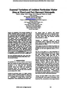
Figure 1. General work flow for PMF analyses of ambient PM species data.

probability function,15,26 potential source contribution function,22,50 cluster analysis,24 and residence time analysis18 are some techniques for analyzing wind trajectories that have been used to aid in the identification of PMF factors. Some studies have augmented PMF results with dispersion modeling of the episodes during which the PM samples were collected. Hedberg et al.29 compared source contributions of local smelters to ambient arsenic concentrations calculated using both PMF and a dispersion model and found dispersion modeling to give a larger source contribution than PMF. Qin and Oduyemi41 used a dispersion model to estimate the contributions of vehicle emissions to ambient PM, because PMF was unable to resolve a profile for motor vehicles, a source known to be present in the airshed under study. Regression of PM source contributions (from the G matrix) onto data collected concurrently with the PM samples can often yield insights into the airshed under study. Previous researchers have regressed the G matrix onto meteorological data; onto gases such as NOx, O3, NH3, and CO; and onto the same PM species used in the PMF model.40,65 All of these regression analyses can aid in identifying the factors output by PMF. In particular, regressing of contributions onto gaseous species can assist in understanding how sources of PM also contribute to the ambient concentrations of gases. Journal of the Air & Waste Management Association 151

Reff, Eberly, and Bhave Table 2. Recommended documentation for analysis of ambient PM data with PMF. Data Preparation Justification and degree of downweighting or reason for excluding • Species • Samples • Individual measurements

Method of uncertainty determination of each measurement used in PMF Calculations of measurements and uncertainties for

PMF Analysis

Solution Interpretation and Analysis

Number of sources • Explore PMF multiple solutions • Justification for best number of factors

Discussion of profile interpretation methods, including citations of all measured source profiles discussed Discussion of any auxiliary quantitative analyses of PMF solutions

Rotational parameters used in final solutions • Fpeak (PMF2) • Fkey (PMF2) • Gkey (PMF2) • Auxiliary Equations (ME) Mode used: robust or nonrobust? Error model if used

• Missing data • Data below detection limits

Q values of final solution: • QTrue or QRobust depending on mode • QTheory Method of apportioning PM mass All goodness of fit measures examined Model uncertainties and methods

CONCLUSIONS Procedures used to identify and apportion sources of ambient PM by fitting a bilinear model (eq 1) to PM species measurements using the PMF algorithm have been reviewed. A procedural diagram amalgamated from this review of PMF applications is shown in Figure 1. The arrows in Figure 1 indicate that the PMF user is encouraged to return to earlier steps if the PMF solution does not fit the data well or if the factors and contributions cannot be adequately physically interpreted. We recommend following this general work flow and documenting all of the procedural details used in future PMF applications as outlined in Table 2. Thorough documentation will especially aid in understanding the challenging step of associating PMF factors with sources of ambient PM, which is largely subjective and sometimes criticized because of undocumented or inconsistent use of species in associating factors with sources. Additionally, if future PMF analyses include calculations and documentation of uncertainties in the modeling results, then the profiles may be compared to see if they are within the uncertainty bounds of each other. This review has also raised a number of questions about the workings of PMF that warrant further research. Previous analyses of trace species in environmental samples have found that different methods for handling data below DL can strongly influence subsequent statistical analyses.68,69 Does this effect apply to PMF analyses of ambient PM species as well? Does duplication of measurements in the data matrix improve or degrade PMF solutions, or is the effect negligible? What is the optimum method of apportioning total PM mass to the different factors resolved by PMF? How do different definitions of uncertainties (␴ij in Table 1), choices of error models, and 152 Journal of the Air & Waste Management Association

values of ␣ affect PMF solutions? What method or combination of methods is optimal for rotating PMF solutions? Is it valid to use the F-key to force factor profiles to resemble emissions speciation profiles? Is G-key useful for rotating PMF solutions? How can the source identification process be improved? Do factor profiles from different studies that are identified as the same source fall within the limits of uncertainty of each other? Is it possible to numerically match profiles resolved by PMF to data in an electronic library of PM source profiles, such as SPECIATE,67 similar to techniques that are often used in the field of spectroscopy?70 The overall goal of the recommended documentation and future research questions is to obtain source apportionment results from PMF that are of known quality. This, in turn, will allow the community to determine which procedural steps give rise to the greatest uncertainty in the modeling results and to find ways to reduce that uncertainty. ACKNOWLEDGMENTS The research presented here was performed under the Memorandum of Understanding between EPA and the U.S. Department of Commerce’s National Oceanic and Atmospheric Administration (NOAA) and under agreement number DW13921548. This work constitutes a contribution to the NOAA Air Quality Program. Although it has been reviewed by EPA and NOAA and approved for publication, it does not necessarily reflect their policies or views. REFERENCES 1. Paatero, P.; Tapper, U. Positive Matrix Factorization: a Non-Negative Factor Model with Optimal Utilization of Error Estimates of Data Values; Envirometrics 1994, 5, 111-126. Volume 57 February 2007

Reff, Eberly, and Bhave 2. Malinowski, E.R. Factor Analysis in Chemistry; John Wiley and Sons, Inc.: New York, NY, 2002. 3. Particulate Matter (PM2.5) Speciation Guidance—Final Draft; U.S. Environmental Protection Agency, Research Triangle Park, NC, 1999; available at: http://www.epa.gov/ttn/amtic/files/ambient/pm25/spec/specfinl. pdf (accessed 2006). 4. Malm, W.C.; Schichtel, B.A.; Pitchford, M.L.; Ashbaugh, L.L.; Eldred, R.A. Spatial and Monthly Trends in Speciated Fine Particle Concentration in the United States. J. Geophys. Res. 2004, 109, DOI 10.1029/ 2003JD003739. 5. Hansen, D.A.; Edgerton, E.S.; Hartsell, B.E.; Jansen, J.J.; Kandasamy, N.; Hidy, G.M.; Blanchard, C.L. The Southeastern Aerosol Research and Characterization Study: Part 1—Overview; J. Air & Waste Manage. Assoc. 2003, 53, 1460-1471. 6. Ramadan, Z.; Song, X.-H.; Hopke, P.K. Identification of Sources of Phoenix Aerosol by Positive Matrix Factorization; J. Air & Waste Manage. Assoc. 2000, 50, 1308-1320. 7. Kim, E.; Hopke, P.K. Source Apportionment of Fine Particles in Washington D.C., Utilizing Temperature-Resolved Carbon Fractions; J. Air & Waste Manage. Assoc. 2004, 54, 773-785. 8. Buzcu, B.; Fraser, M.P.; Kulkarni, P.; Chellam, S. Source Identification and Apportionment of Fine Particulate Matter in Houston, TX, Using Positive Matrix Factorization; Environ. Eng. Sci. 2003, 20, 533-545. 9. Huang, S.; Rahn, K.A.; Arimoto, R. Testing and Optimizing Two FactorAnalysis Techniques on Aerosol at Narragansett, Rhode Island; Atmos. Environ. 1999, 33, 2169-2185. 10. Ito, K.; Xue, N.; Thurston, G. Spatial Variation of PM2.5 Chemical Species and Source-Apportioned Mass Concentrations in New York City; Atmos. Environ. 2004, 38, 5269-5282. 11. Li, Z.; Hopke, P.K.; Husain, L.; Qureshi, S.; Dutkiewicz, V.A.; Schwab, J.J.; Drewnick, F.; Demerjian, K.L. Sources of Fine Particle Composition in New York City; Atmos. Environ. 2004, 38, 6521-6529. 12. Maykut, N.N.; Lewtas, J.; Kim, E.; Larson, T.V. Source Apportionment of PM2.5 at an Urban IMPROVE Site in Seattle, Washington; Environ. Sci. Technol. 2003, 37, 5135-5142. 13. Kim, E.; Hopke, P.K.; Edgerton, E.S. Improving Source Identification of Atlanta Aerosol Using Temperature Resolved Carbon Fractions in Positive Matrix Factorization; Atmos. Environ. 2004, 38, 3349-3362. 14. Kim, E.; Hopke, P.K.; Paatero, P.; Edgerton, E.S. Incorporation of Parametric Factors into Multilinear Receptor Model Studies of Atlanta Aerosol; Atmos. Environ. 2003, 37, 5009-5021. 15. Kim, E.; Hopke, P.K.; Edgerton, E.S. Source Identification of Atlanta Aerosol by Positive Matrix Factorization; J. Air & Waste Manage. Assoc. 2003, 53, 731-739. 16. Liu, W.; Wang, Y.; Russell, A.; Edgerton, E.S. Atmospheric Aerosol over Two Urban-Rural Pairs in the Southeastern United States: Chemical Composition and Possible Sources; Atmos. Environ. 2005, 39, 44534470. 17. Ogulei, D.; Hopke, P.K.; Zhou, L.; Paatero, P.; Park, S.S.; Ondov, J.M. Receptor Modeling for Multiple Time Resolved Species: the Baltimore Supersite; Atmos. Environ. 2005, 39, 3751-3762. 18. Poirot, R.L.; Wishinski, P.R.; Hopke, P.K.; Polissar, A.V. Comparative Application of Multiple Receptor Methods to Identify Aerosol Sources in Northern Vermont; Environ. Sci. Technol. 2001, 35, 4622-4636. 19. Polissar, A.V.; Hopke, P.K.; Poirot, R.L. Atmospheric Aerosol over Vermont: Chemical Composition and Sources; Environ. Sci. Technol. 2001, 35, 4604-4621. 20. Polissar, A.V.; Hopke, P.K.; Paatero, P.; Malm, W.C.; Sisler, J.F. Atmospheric Aerosol over Alaska 2. Elemental Composition and Sources; J. Geophys. Res. 1998, 103, 19045-19057. 21. Kim, E.; Larson, T.V.; Hopke, P.K.; Slaughter, C.; Sheppard, L.E.; Claiborn, C. Source Identification of PM2.5 in an Arid Northwest U.S. City by Positive Matrix Factorization; Atmos. Res. 2003, 66, 291-305. 22. Liu, W.; Hopke, P.K.; Han, Y.-J.; Yi, S.-M.; Holsen, T.M.; Cybart, S.; Kozlowski, K.; Milligan, M. Application of Receptor Modeling to Atmospheric Constituents at Potsdam and Stockton, NY; Atmos. Environ. 2003, 37, 4997-5007. 23. Kim, E.; Hopke, P.K. Improving Source Identification of Fine Particles in a Rural Northeastern U.S. Area Utilizing Temperature-Resolved Carbon Fractions. J. Geophys. Res. 2004, 109, DOI 10.1029/ 2003JD004199. 24. Lee, J.H.; Yoshida, Y.; Turpin, B.J.; Hopke, P.K.; Poirot, R.L.; Lioy, P.J.; Oxley, J.C. Identification of Sources Contributing to Mid-Atlantic Regional Aerosol; J. Air & Waste Manage. Assoc. 2002, 52, 1186-1205. 25. Zhao, W.; Hopke, P.K. Source Apportionment for Ambient Particles in the San Gorgonio Wilderness; Atmos. Environ. 2004, 38, 5901-5910. 26. Begum, B.A.; Kim, E.; Biswas, S.K.; Hopke, P.K. Investigation of Sources of Atmospheric Aerosol at Urban and Semi-Urban Areas in Bangladesh; Atmos. Environ. 2004, 38, 3025-3038. 27. Chueinta, W.; Hopke, P.K.; Paatero, P. Investigation of Sources of Atmospheric Aerosol at Urban and Suburban Residential Areas of Thailand by Positive Matrix Factorization; Atmos. Environ. 2000, 34, 3319-3329. Volume 57 February 2007

28. Gong, S.L.; Barrie, L.A. Trends of Heavy Metal Components in the Arctic Aerosols and Their Relationship to the Emissions in the Northern Hemispere; Sci. Total Environ. 2005, 342, 175-183. 29. Hedberg, E.; Gidhagen, L.; Johansson, C. Source Contributions to PM10 and Arsenic Concentrations in Central Chile Using Positive Matrix Factorization; Atmos. Environ. 2005, 39, 549-561. 30. Hien, P.D.; Bac, V.T.; Thinh, N.T.H. PMF. Receptor Modelling of Fine and Coarse PM10 in Air Masses Governing Monsoon Conditions in Hanoi, Northern Vietnam; Atmos. Environ. 2004, 38, 189-201. 31. Huang, S.; Arimoto, R.; Rahn, K.A. Sources and Source Variations for Aerosol at Mace Head, Ireland; Atmos. Environ. 2001, 35, 1421-1437. 32. Yuan, Z.; Lau, A.K.H.; Zhang, H.; Yu, J.Z.; Louie, P.K.K.; Fung, J.C.H. Identification and Spatiotemporal Variations of Dominant PM10 Sources over Hong Kong; Atmos. Environ. 2006, 40, 1803-1815. 33. Yuan, Z.B.; Yu, J.Z.; Lau, A.K.H., Louie, P.K.K., Fung, J.C.H;. Application of Positive Matrix Factorization in Estimating Aerosol Secondary Organic Carbon in Hong Kong and Its Relationship with Secondary Sulfate; Atmos. Chem. Physics 2006, 6, 25-34. 34. Lee, E.; Chan, C.K.; Paatero, P. Application of Positive Matrix Factorization in Source Apportionment of Particulate Pollutants in Hong Kong; Atmos. Environ. 1999, 33, 3201-3212. 35. Tsai, J.; Owega, S.; Evans, G.; Jervis, R.; Fila, M.; Tan, P.; Malpica, O. Chemical Composition and Source Apportionment of Toronto Summertime Urban Fine Aerosol (PM2.5); J. Radioanal. Nucl. Chem. 2004, 259, 193-197. 36. Lee, P.K.H., Brook, J.R.; Dabek-Zlotorzynska, E.; Mabury, S. Identification of the Major Sources Contributing to PM2.5 Observed in Toronto; Environ. Sci. Technol. 2003, 37, 4831-4840. 37. Lei, C.; Landsberger, S.; Basunia, S.; Tao, Y. Study of PM2.5 in Beijing Suburban Site by Neutron Activation Analysis and Source Apportionment; J. Radioanal. Nucl. Chem. 2004, 261, 87-94. 38. Sun, Y.; Zhuang, G.; Wang, Y.; Han, L.; Guo, J.; Dan, M.; Zhang, W.; Wang, Z.; Hao, Z. The Air-Borne Particulate Pollution in Beijing— Concentration, Composition, Distribution and Sources; Atmos. Environ. 2004, 38, 5991-6004. 39. Prendes, P.; Andrade, J.M.; Lopez-Mahia, P.; Prada, D. Source Apportionment of Inorganic Ions in Airborne Urban Particles from Coruna City (N.W. of Spain) Using Positive Matrix Factorization; Talanta 1999, 49, 165-178. 40. Wang, H.; Shooter, D. Source Apportionment of Fine and Coarse Atmospheric Particles in Auckland, New Zealand; Sci. Total Environ. 2005, 340, 189-198. 41. Qin, Y.; Oduyemi, K. Atmospheric Aerosol Source Identification and Estimates of Source Contributions to Air Pollution in Dundee, UK; Atmos. Environ. 2003, 37, 1799-1809. 42. Yli-Tuomi, T.; Paatero, P.; Raunemaa, T. The Soil Factor in Rautavaara Aerosol in Positive Matrix Factorization Solutions with 2 to 8 Factors; J. Aerosol Sci. 1996, 27, S671–S672. 43. Hien, P.D.; Bac, V.T.; Thinh, N.T.H. Investigation of Sulfate and Nitrate Formation on Mineral Dust Particles by Receptor Modeling; Atmos. Environ. 2005, 39, 7231-7239. 44. Paatero, P. The Multilinear Engine—a Table-Driven, Least Squares Program for Solving Multilinear Problems, Including the N-Way Parallel Factor Analysis Model; J. Computat. Graph. Stat. 1999, 8, 854-888. 45. EPA PMF 1.1 User’s Guide; U.S. Environmental Protection Agency, Research Triangle Park, NC, 2004; available at: http://www.epa.gov/ heasd/products/pmf/pmf.htm (accessed 2006). 46. Polissar, A.V.; Hopke, P.K.; Malm, W.C.; Sisler, J.F. The Ratio of Aerosol Optical Absorption Coefficients to Sulfur Concentrations, as an Indicator of Smoke from Forest Fires when Sampling in Polar Regions; Atmos. Environ. 1996, 30, 1147-1157. 47. Kim, E.; Hopke, P.K.; Qin, Y. Estimation of Organic Carbon Blank Values and Error Structures of the Speciation Trends Network Data for Source Apportionment; J. Air & Waste Manage. Assoc. 2005, 55, 11901199. 48. Kim, E.; Hopke, P.K.; Kenski, D.M.; Koerber, M. Sources of Fine Particles in a Rural Midwestern U.S. Area; Environ. Sci. Technol. 2005, 39, 4953-4960. 49. Sirois, A.; Barrie, L.A. Arctic Lower Tropospheric Aerosol Trends and Composition at Alert, Canada: 1980 –1995; J. Geophys. Res. 1999, 104, 11599-11618. 50. Kim, E.; Hopke, P.K. Improving Source Apportionment of Fine Particles in the Eastern United States Utilizing Temperature-Resolved Carbon Fractions; J. Air & Waste Manage. Assoc. 2005, 55, 1456-1463. 51. Chow, J.C.; Watson, J.G.; Pritchett, L.C.; Pierson, W.R.; Frazier, C.A.; Purcell, R.G. The DRI Thermal/Optical Reflectance Carbon Analysis System: Description, Evaluation and Application in US Air Quality Studies; Atmos. Environ. 1993, 27A, 1185-1201. 52. Song, X.H.; Faber, N.M.; Hopke, P.K.; Seuss, D.T.; Prather, K.A.; Schauer, J.J.; Cass, G.R. Source Apportionment of Gasoline and Diesel by Multivariate Calibration Based on Single Particle Mass Spectral Data; Anal. Chim. Acta 2001, 446, 327-343. 53. Paatero, P.; Hopke, P.K. Discarding or Downweighting High-Noise Variables in Factor Analytic Models; Anal. Chim. Acta 2003, 490, 277-289. Journal of the Air & Waste Management Association 153

Reff, Eberly, and Bhave 54. Kim, E.; Hopke, P.K.; Larson, T.V.; Maykut, N.N.; Lewtas, J. Factor Analysis of Seattle Fine Particles; Aerosol Sci. Technol. 2004, 38, 724738. 55. Liu, W.; Hopke, P.K.; VanCuren, R.A. Origins of Fine Aerosol Mass in the Western United States Using Positive Matrix Factorization; J. Geophys. Res. 2003, 108, DOI 10.1029/2003JD003678. 56. Paatero, P. User’s Guide for the Multilinear Engine Program “ME2” for Fitting Multilinear and Quasi-Multilinear Models; University of Helsinki: Helsinki, Finland, 2000. 57. Paatero, P. User’s Guide for Positive Matrix Factorization Programs PMF2 and PMF3; University of Helsinki: Helsinki, Finland, 2004. 58. Han, J.; Moon, K.; Lee, S.; Kim, Y.; Ryu, S.; Cliff, S.; Yi, S. Size-Resolved Source Apportionment of Ambient Particles by Positive Matrix Factorization at Gosan Background Site in East Asia; Atmos. Chem. Physics 2006, 6, 211-223. 59. Yli-Tuomi, T.; Hopke, P.K.; Paatero, P.; Basunia, M.S.; Landsberger, S.; Viisanen, Y.; Paatero, J. Atmospheric Aerosol over Finnish Arctic: Source Analysis by the Multilinear Engine and the Potential Source Contribution Function; Atmos. Environ. 2003, 37, 4381-4392. 60. Henry, R.C. Current Factor Analysis Receptor Models Are Ill-Posed; Atmos. Environ.1987, 21, 1815-1820. 61. Paatero, P.; Hopke, P.K.; Song, X.-H.; Ramadan, Z. Understanding and Controlling Rotations in Factor Analytic Models; Chemometrics Intell. Lab. Systems 2002, 60, 253-264. 62. Paatero, P.; Hopke, P.K.; Begum, B.A.; Biswas, S.K. A Graphical Diagnostic Method for Assessing the Rotation in Factor Analytical Models of Atmospheric Pollution; Atmos. Environ. 2005, 39, 193-201. 63. Begum, B.A.; Hopke, P.K.; Zhao, W. Source Identification of Fine Particles in Washington, DC, by Expanded Factor Analysis Modeling; Environ. Sci. Technol. 2005, 39, 1129-1137. 64. Paatero, P.; Hopke, P.K;. Utilizing Wind Direction and Wind Speed as Independent Variables in Multilinear Receptor Modeling Studies; Chemometrics Intell. Lab. Systems 2002, 60, 25-41. 65. Zhou, L.; Hopke, P.K.; Paatero, P.; Ondov, J.M.; Pancras, J.P.; Pekney, N.J.; Davidson, C.I. Advanced Factor Analysis for Multiple Time Resolution Aerosol Composition Data; Atmos. Environ. 2004, 38, 49094920. 66. Efron, B.; Tibshirani, R.J. An Introduction to the Bootstrap; Chapman and Hall: New York, NY, 1993.

154 Journal of the Air & Waste Management Association

67. Beck, L. SPECIATE—EPA’s Database of Speciated Emission Profiles. In Proceedings of A&WMA’s 99th Annual Conference and Exhibition, Healthy Environments: Rebirth & Renewal, New Orleans, June 20 –23, 2006; Paper No. 229. 68. Dakins, M.E.; Porter, P.S.; West, M.; Rao, S.T. Using Uncensored TraceLevel Measurements to Detect Trends in Ground Water Contamination; Water Resources Bull. 1996, 32, 799-805. 69. Rao, S.T.; Ku, J.-Y.; Rao, K.S. Analysis of Toxic Air Contaminant Data Containing Concentrations below the Limit of Detection; J. Air & Waste Manage. Assoc. 1991, 41, 442-448. 70. Bjerga, J.M.; Small, G.W. Automated Selection of Library Subsets for Infrared Spectral Searching; Anal. Chem. 1990, 62, 226-233. 71. Xie, Y.-L.; Hopke, P.K.; Paatero, P.; Barrie, L.A.; Li, S.-M. Identification of Source Nature and Seasonal Variations of Arctic Aerosol by the Multilinear Engine; Atmos. Environ. 1999, 33, 2549-2562.

About the Authors Adam Reff is a postdoctoral fellow in both the Atmospheric Modeling Division and the Human Exposure and Atmospheric Sciences Division of the National Exposure Research Laboratory of U.S. Environmental Protection Agency (EPA). Shelly Eberly is a statistician with EPA. Prakash Bhave is a physical scientist with National Oceanic and Atmospheric Administration. Address correspondence to: Adam Reff, U.S. Environmental Protection Agency, Mail Code E243-03, Research Triangle Park, NC 27711; phone: ⫹1-919-541-5683; fax: ⫹1-919-541-1379; e-mail: Reff. [email protected].

Volume 57 February 2007