For technical support beyond the call of duty - Anne Zanotti, Brian Marriott, ... networks to a complex real-world problem such as sign language recognition.
Recognition of Sign Language Using Neural Networks
by Peter Wray Vamplew B.A, B.Sc. (Hons.), Flinders University of South Australia (1990) Submitted in fulfilment of the requirements for the degree of Doctor of Philosophy University of Tasmania May 1996
i
This thesis contains no material which has been accepted for a degree or diploma by the University of Tasmania or any other institution, except by way of background information which is duly acknowledged in the thesis. To the best of my knowledge and belief no material previously published or written by another person is included, except where due acknowledgment is made in the text of the thesis.
ii
This thesis may be made available for loan and limited copying in accordance with the Copyright Act 1968.
iii
This work is dedicated to my parents in appreciation of the love and support they have given to me. In particular I wish to thank them for encouraging me to move to Tasmania when the opportunity presented itself.
iv
Acknowledgments I wish to thank my supervisor Dr Tony Adams for always being there to bounce ideas off, and for helping me through the dark days when this project seemed an impossibility. Also thanks to Mr Phil Collier for his assistance with C4.5 and the preparation of this thesis. Thankyou to all of my friends and family for their support and understanding, and particularly to Sandy. Without them I doubt this work would have been completed. Many other people deserve thanks for the contributions they have made to this research over the past five years. The following list is far from exhaustive, and I greatly appreciate the efforts of everyone who has helped me. For being an endless source of good ideas, technical knowhow and distractions – my fellow students from the Artificial Neural Networks Research Group, particularly Carl Lewis, Sam Waugh, Lee Arnould and Tim Freeman. For additional distractions, the lolly drawer and stealing our lab – the CDG postgrads (Richard Gregg, Richard Cockerill, Nicole Clark and David Herbert). For technical support beyond the call of duty - Anne Zanotti, Brian Marriott, Ross Richardson, Terry Bigwood, Wei Shang, Rick Field, Andrew 'Buggs' Routley and James Graham. Believe me – these people have earned their keep! For sharing their knowledge with me, either face to face or via the Internet Peter Bailey and Peter Cippone of the Tasmanian Deaf Society, Anne Potter, Trevor Johnston, Dave Moscowitz, Jim Kramer, Sidney Fels, Warren Robinette, Mike Gigante, Geoff Roberts, Shirley Peters, Eun-Jung Holden, Scott Fahlman, Jeffrey Elman, Tony Robinson and the many others whose names have disappeared into the black hole that is my electronic mailbox.
v
Abstract This thesis details the development of a computer system (labelled the SLARTI system) capable of recognising a subset of signs from Auslan (the sign language of the Australian Deaf community), based on the pattern classification paradigm of artificial neural networks. The research discussed in this work has two main streams. The first is the creation of a practical sign classification system, suitable for use within a sign language training system or other applications based on hand gestures. The second is an exploration of the suitability of neural networks for the creation of a real-time classification system with the ability to process temporal patterns. Sign languages such as Auslan are the primary form of communication between members of the Deaf community. However these languages are not widely known outside of these communities, and hence a communications barrier can exist between Deaf and hearing people. The techniques for recognising signs developed in this research allow the creation of systems which can help to eliminate this barrier, either by providing computer tools to assist in the learning of sign language, or potentially the creation of portable sign-language-to-speech translation systems. Artificial neural networks have proved to be an extremely useful approach to pattern classification tasks, but much of the research in this field has concentrated on relatively simple problems. Attempting to apply these networks to a complex real-world problem such as sign language recognition exposed a range of issues affecting this classification technique. The development of the SLARTI system inspired the creation of several new techniques related to neural networks, which have general applicability beyond this particular application. This thesis includes discussion of techniques related to issues such as input encoding, improving network generalisation, training recurrent networks and developing modular, extensible neural systems.
vi
Contents 1 Introduction................................................................................................................ 1 1.1 Thesis Description ............................................................................................. 1 1.2 Justification......................................................................................................... 1 1.2.1 Benefits to the Deaf community.......................................................... 1 1.2.2 Benefits to neural networks research.................................................. 2 1.3 Research Goals................................................................................................... 3 1.3.1 Sign language and gesture recognition.............................................. 3 1.3.2 Neural networks.................................................................................... 4 1.4 Thesis Layout ..................................................................................................... 4 1.5 Acknowledgments............................................................................................. 6 1.6 Publications arising from this work................................................................ 6 2 Sign language............................................................................................................. 8 2.1 Introduction to sign language ......................................................................... 8 2.2 Structural components of signs ....................................................................... 12 2.3 Components of Auslan signs........................................................................... 15 2.3.1 Auslan handshapes ............................................................................... 15 2.3.3 Auslan hand orientations..................................................................... 18 2.3.3 Auslan hand locations .......................................................................... 19 2.3.4 Auslan hand motions............................................................................ 19 3 Hand-sensing technology......................................................................................... 21 3.1 Measuring joint positioning............................................................................. 21 3.1.1 Instrumented gloves ............................................................................. 21 3.1.2 Camera based joint measurement....................................................... 24 3.2 Position tracking................................................................................................ 26 3.2.1 Mechanical systems............................................................................... 26 3.2.2 Optical systems...................................................................................... 27 3.2.3 Acoustic systems.................................................................................... 27 3.2.4 Magnetic systems .................................................................................. 28 3.2.5 Comparison of position sensing technologies................................... 29 3.3 Sensing technology used for the SLARTI project ......................................... 30 3.3.1 Selection of sensing technology........................................................... 30 3.3.2 The CyberGlove..................................................................................... 32 3.3.3 The Polhemus 3Space IsoTrak............................................................. 33 4 Hand gesture recognition......................................................................................... 35 4.1 Glove-based gesture recognition systems...................................................... 36 4.1.1 Glove-Talk .............................................................................................. 36 vii
4.1.2 Glove-TalkII............................................................................................ 37 4.1.3 The Talking Glove ................................................................................. 39 4.1.4 GIVEN..................................................................................................... 41 4.1.5 NTT/ATR Japanese manual alphabet recognition system ............. 42 4.1.6 University of Nebraska-Lincoln handshape recognition system..................................................................................................... 43 4.1.7 Waseda University musical conducting gesture recognition system ............................................................................... 44 4.1.8 Fujitsu Japanese sign-language recognition system......................... 45 4.1.9 Royal Melbourne Institute of Technology gesture recognition system ............................................................................... 47 4.1.10 GloveTalker .......................................................................................... 49 4.1.11 University of Milan sign recognition system .................................. 50 4.1.12 MIT Coverbal Gesture Recognition system..................................... 51 4.2 Camera-based gesture recognition systems .................................................. 52 4.2.1 Sign Motion Understanding (SMU) system ..................................... 52 4.2.2 Simon Fraser University ASL translation system............................. 54 4.2.4 University of Central Florida gesture recognition system .............. 55 4.3 Comparison and summary of existing systems............................................ 57 4.4 Applications of hand gesture recognition ..................................................... 59 4.4.1 Sign language translation system ....................................................... 59 4.4.2 Sign language training system ............................................................ 61 4.4.3 Gesture driven interfaces ..................................................................... 62 5 Spatial neural networks............................................................................................ 66 5.1 What are neural networks? .............................................................................. 66 5.2 Networks used for this research...................................................................... 67 5.2.1 Activation functions.............................................................................. 68 5.2.2 Network architecture ............................................................................ 68 5.2.3 Input and output encodings ................................................................ 71 5.2.4 Learning algorithms.............................................................................. 71 5.2.5 Measuring the length of training ........................................................ 73 5.2.6 Terminating the training process ........................................................ 75 5.3 Properties of neural networks ......................................................................... 76 5.3.1 Learning from examples, generalisability and pattern recognition............................................................................................. 76 5.3.2 Scaling ..................................................................................................... 77 5.3.3 Plasticity and incremental learning .................................................... 77 5.3.4 Distributed representation ................................................................... 78 5.3.5 Parallel implementation ....................................................................... 79
viii
6 Temporal neural networks....................................................................................... 80 6.1 Processing sequences with neural networks................................................. 80 6.2 Non-recurrent architectures for temporal processing.................................. 81 6.2.1 Tapped delay lines ................................................................................ 81 6.2.2 Time Delay Neural Networks.............................................................. 84 6.3 Recurrent architectures for temporal processing.......................................... 87 6.3.2 Elman network....................................................................................... 87 6.3.2 Jordan network ...................................................................................... 88 6.3.3 General transformed output and state (TOS) network.................... 89 6.4 Recurrent training algorithms ......................................................................... 91 6.4.1 Simple Recurrent Network (SRN)....................................................... 91 6.4.2 Backpropagation Through Time (BPTT)............................................ 92 6.4.3 Real-Time Recurrent Learning (RTRL) .............................................. 95 7 Neural network techniques...................................................................................... 97 7.1 Generalisation and uncertainty in neural networks..................................... 97 7.1.1 Data set.................................................................................................... 97 7.1.2 Improving generalisation.................................................................... 98 7.1.3 Dealing with uncertainty in classification ......................................... 101 7.2 Applying thresholds to temporal sequences................................................ 104 7.3 Missing values and neural networks.............................................................. 106 7.3.1 Techniques for handling missing values ........................................... 107 7.3.2 Experiments and results for single missing values .......................... 111 7.3.3 Experiments and results for multiple missing values...................... 112 7.3.4 Conclusions ............................................................................................ 113 7.4 Representing cyclical data................................................................................ 115 7.4.1 Encoding cyclical data .......................................................................... 116 7.4.2 Classification using cyclic input data ................................................. 118 7.4.3 Decoding cyclical data .......................................................................... 122 7.4.4 Comparison of decoding methods...................................................... 124 7.5 BPTT and Neural Transplant Surgery............................................................ 126 7.5.1 Background and data sets .................................................................... 126 7.5.2 Neural Transplant Surgery .................................................................. 127 7.5.3 Experimental conditions and results .................................................. 129 8 Design of the SLARTI system.................................................................................. 132 8.1 Modularity as a solution to scalability problems.......................................... 132 8.2 Modularity as a solution to plasticity problems ........................................... 133 8.3 Modular design of the SLARTI system .......................................................... 134 9 Classifying spatial features of signs........................................................................ 136 9.1 Classifying handshape...................................................................................... 136 ix
9.1.1 Data gathering........................................................................................ 136 9.1.2 Output encoding.................................................................................... 137 9.1.3 Calibration.............................................................................................. 138 9.1.3 Comparison to other learning methods ............................................. 141 9.2 Classifying hand orientation............................................................................ 142 9.2.1 Data gathering........................................................................................ 142 9.2.2 Network structure ................................................................................. 143 9.2.3 Error measurement................................................................................ 144 9.2.4 Results ..................................................................................................... 145 9.3 Classifying hand location................................................................................. 147 9.3.1 Data gathering and calibration............................................................ 147 9.3.2 Network structure ................................................................................. 147 9.3.3 Error measurement................................................................................ 148 9.3.4 Results ..................................................................................................... 149 9.3.5 Possible improvements......................................................................... 151 10 Classification of hand motion................................................................................ 153 10.1 Prototype hand-motion classification network........................................... 153 10.1.1 Data gathering...................................................................................... 153 10.1.2 Network architecture .......................................................................... 154 10.1.3 Recognition results.............................................................................. 154 10.2 Creation of the final hand-motion classification network......................... 155 10.2.1 Data gathering...................................................................................... 155 10.2.2 Classification with a recurrent network........................................... 156 10.2.3 Classification with a non-recurrent network................................... 157 11 Classification of signs.............................................................................................. 159 11.1 Development of a sign classifier.................................................................... 159 11.1.1 Selection of the best feature-extraction networks........................... 159 11.1.2 Selection of the vocabulary ................................................................ 160 11.1.3 Data gathering...................................................................................... 161 11.1.4 The unsuitability of neural networks for the final classifier.................................................................................................. 162 11.1.5 Nearest neighbours ............................................................................. 163 11.1.6 C4.5 ........................................................................................................ 166 11.1.7 Reducing the misclassification rate................................................... 167 11.1.8 Segmentation of continuous signs .................................................... 169 11.2 The final SLARTI system................................................................................ 179 11.2.1 SLARTI system structure and performance .................................... 179 11.2.2 Comparison to other gesture-recognition systems......................... 181 11.2.3 Potential applications of SLARTI...................................................... 183 x
12 Conclusion................................................................................................................ 186 12.1 The SLARTI system......................................................................................... 186 12.2 Neural network techniques............................................................................ 187 12.2.1 System architecture ............................................................................. 187 12.2.2 Neural network techniques................................................................ 188 References...................................................................................................................... 190 Appendix 1 Heuristic distance measure ................................................................... 202 Appendix 2 Glossary.................................................................................................... 205 Appendix 3 List of abbreviations............................................................................... 207
xi
xii
1 Introduction 1.1 Thesis Description The aim of this research is to develop a prototype system for the automatic recognition of sign language, based on a series of artificial neural networks. For reference purposes this system is dubbed the SLARTI (Sign LAnguage RecogniTIon) system.
1.2 Justification The research is motivated by two contrasting but complementary goals. The first is that a sign language system would be potentially beneficial in aiding communication between members of the Deaf community and the hearing community. The second is that the process of developing such a system using neural networks gives opportunities for studying and extending the networks themselves. 1.2.1 Benefits to the Deaf community The first motivating factor is the possibility of reducing the communications barrier which exists between the deaf and hearing communities. The problems that deaf people encounter in trying to communicate with the general community are well documented (see for example Moscovitz and Walton 1990). Moscovitz and Walton use the term 'deaf' in two distinct senses distinguished by whether the word is capitalised or not. In its uncapitalised form 'deaf' refers purely to an individual's ability to hear, as it would be used in common parlance. The capitalised form 'Deaf' is used to indicate the cultural aspects of being deaf. This convention is also used within this thesis. In many ways the Deaf community is similar to an ethnic community in that they form a subgroup within society, complete with its own culture and language (in this case sign language)1. People who become deaf later in life after learning a spoken language in general do not use sign language as much and are less involved in the Deaf community than those whose hearing loss occurred earlier in life. The inability to hear means that many deaf people do not develop good skills in the English language and prefer not to use it. This is because the sign languages most commonly used within the
1
Kerridge (1995) provides a very interesting discussion of the importance placed on Deaf culture by the Deaf community.
1
Deaf community are not grammatically related to English – an issue which is discussed in more detail in Chapter 2. In addition very few hearing people have much knowledge of sign language, and so communication between sign-language users and hearing people poses many problems. For this reason the Deaf community tends to be insular and somewhat separate from the rest of society. When it is necessary to communicate with hearing people (for example when shopping) signers often have to resort to pantomimic gestures or written notes to communicate their needs, and many are uncomfortable even in using notes due to their lack of English writing skills. An automated sign language translation system would help to break down this communication barrier (in much the same way that an automated English-to-French translator would help Australian tourists visiting Paris to communicate). Ideally such a system should allow signers to use their native sign language, as this language is an integral component of Deaf culture. As discussed in Chapter 4 the aim of this project is not to develop a full sign language to English translation system; such a task is too large and complex to attempt at this stage. Instead the aim is to create a prototype system for the recognition of signs, and in so doing develop techniques which could later be incorporated into a more complete translation system. It is also envisioned that the system developed could be adapted for use as a training tool to aid hearing people attempting to learn sign language. 1.2.2 Benefits to neural networks research The second reason for undertaking this research is that the problem of recognising signs is seen as being an interesting driving problem for neural networks research. A large proportion of neural networks research has been performed on 'toy' or contrived problems which may bear little relevance to real-world tasks. Whilst this research has been invaluable in developing the basic techniques used in neural networks, attempting to apply these techniques to a real problem is seen as likely to produce new insights into neural network methodologies. In particular the temporal component involved in signing forms a challenging task for neural networks as the majority of research so far has been focussed on purely static problems. Attempting to address this aspect of signing aims to yield insights into the methods of extending neural networks to this temporal domain. 2
These twin motivating factors influence the directions taken during this research, and are reflected in this thesis which addresses both the performance of the final system for recognising signs, and also the issues related to neural networks arising from the development of this system.
1.3 Research Goals Clearly the aims of this research also reflect the two factors motivating the work, and therefore need to be discussed separately. 1.3.1 Sign language and gesture recognition One aim of this research is to improve on the results obtained by previous work on hand-gesture and sign-language recognition. As discussed in the review of this work presented in Chapter 4, existing systems have two main shortcomings, namely a relatively small vocabulary and a capacity to recognise only static hand shapes or simple motions. Development of the SLARTI system is focussed on improvements in these areas. Previous systems have generally supported only a relatively small vocabulary (being the number of signs or gestures recognised) and the size and contents of the vocabulary are fixed. One of the main goals of this research is a desire to design the system in a manner which will allow the vocabulary to be extended in the future without requiring major modification of the system. The second goal is to increase the complexity of the signs recognised, particularly with regard to their motion component. The majority of the research into hand-gesture recognition has concentrated on static hand configurations or very simple motions, rather than the potentially complicated movements involved in Deaf sign languages. A further problem which has been rarely researched is the automatic segmentation of signs from within a continuous sequence of signing. Most systems developed so far have dealt only with individual signs and therefore have not addressed the issue of distinguishing the end of one sign from the start of the next sign. The ability to handle continuous signing will be a fundamental quality of any practical sign-language recognition system. Although it is considered to be outside the primary scope of this thesis, a possible method of tackling this problem arises naturally out of the 3
development of the system. Therefore some preliminary results are included amongst the discussion of future work in Chapter 11. 1.3.2 Neural networks The goals related to the use of neural networks are less easily defined in advance, as it is not possible to anticipate the specific issues which would arise during the development of the system. However there are some general issues which could be seen as likely to be encountered during this development process. The first of these issues is the modular use of neural networks to overcome problems of scaling. The problem being tackled is extremely large and previous neural networks research has indicated that the use of a single network would not be appropriate. Therefore SLARTI consists of several networks, and the connection together of these to form the final system is one issue which the research is intended to address. The second issue is the use of neural networks to recognise temporal patterns. As described above one of the goals related to gesture recognition is the recognition of complex hand motions, and therefore it is necessary to consider how neural networks can be extended from the relatively wellexplored domain of spatial pattern processing to handle spatio-temporal patterns.
1.4 Thesis Layout The chapters of this thesis can be divided into four logical sections. • Chapters 2 to 4 provide background information on the field of sign language and hand-gesture recognition. • Chapter 2 gives information about sign languages in general, and Australian Sign Language (Auslan) in particular. It discusses the general features of manual languages, and also those aspects which are of most direct relevance for the development of computerised recognition systems. • Chapter 3 discusses the various types of hardware which can be used to capture the data necessary to recognise signs and hand gestures. The various options are evaluated, and the hardware used for this system is described in more detail. 4
• Chapter 4 describes previous work done in the area of computer recognition of sign language and hand gestures, and outlines how the SLARTI system developed in this thesis differs from these previous systems. • Chapters 5 and 6 also provide background information, in this case relating to neural networks, which are the primary form of pattern recognition used in this research. • Chapter 5 discusses the use of neural networks for recognition of spatial patterns. It commences with a discussion of neural networks in general, focusing on the feed-forward networks used for this work. Particular attention is payed to aspects of this style of network which are of most relevance for the SLARTI project. • Chapter 6 discusses the extension to the temporal domain of the spatial networks examined in the previous chapter. Existing architectures and learning algorithms are reviewed and compared, in the light of the requirements of the SLARTI project. • Chapter 7 can be seen as forming the third section of this thesis. It deals with issues related to neural networks which arise out of the application of these networks to the task of sign language recognition. As such it does not relate directly to the SLARTI system, although many of the techniques described in this chapter are incorporated into the final system. • Chapters 8 through 11 detail the creation of the SLARTI system, explaining how the techniques outlined in Chapters 5, 6 and 7 were utilised in creating the final system. • Chapter 8 describes the overall structure of the SLARTI system, and provides the rationale for the modular design of the system with respect to the limitations of neural networks covered in Chapters 5 and 6. • Chapter 9 deals with the application of spatial neural network techniques to the classification of three of the manual features of Auslan signing (handshape, orientation and place of articulation).
5
• Chapter 10 covers the application of temporal neural network techniques to the classification of the motion component of Auslan signs. • Chapter 11 describes how the various networks detailed in Chapters 9 and 10 are linked together to form the final SLARTI system. It analyses the overall performance of this system on non-continuous signs, and provides some preliminary investigations into extending the system to the domain of continuous signs.
1.5 Acknowledgments The funding for the hand-sensing equipment used in this research was jointly provided by a New Staff Priming Grant from the University of Tasmania, and an internal grant from the Department of Computer Science. The 486 PC on which SLARTI was developed was provided by the Artificial Neural Networks Research Group.
1.6 Publications arising from this work A number of refereed publications have been produced as a result of this research. The following list provides details of these publications, as well as indicating the sections of the thesis to which they correspond. Vamplew, P., Computer Recognition of Sign Language, Proceedings of Paper Clips to Silicon Chips: Second National Conference on Disability Issues and Technology, Hobart, 6-9 October 1991 (Chapters 2, 4 and 8) Vamplew, P. and Adams, A, Missing Values in a Backpropagation Neural Net, Proceedings of ACNN'92: The Third Australian Conference on Neural Networks, Canberra, 3-5 February 1992 (Chapter 7.3) Vamplew, P. and Adams, A, The SLARTI System: Applying Artificial Neural Networks to Sign Language Recognition, Proceedings of the Conference on Technology and Persons with Disabilities, California State University, Northridge, 18-21 March, 1992 (Chapters 7.1 and 8) Vamplew, P., The SLARTI Sign Language Recognition System: A Progress Report, Proceedings of the Australian Conference on Technology and People With Disabilities, Regency Park Centre for the Young Disabled, Adelaide, 5-7 July 1993 (Chapters 8 and 9.1)
6
Vamplew, P. and Adams, A, Neural Transplant Surgery: An Approach to Pre-training Recurrent Networks, Proceedings of the Fifth Australian Conference on Neural Networks, University of Queensland, February 1994 (Chapter 7.5) Vamplew, P. and Adams, A, Recognition and Anticipation of Hand Motions Using a Recurrent Neural Network, Proceedings of the IEEE International Conference on Neural Networks, Perth, Western Australia, 27 November - 1 December 1995 (Chapters 10.1 and 11.1.8) Vamplew, P., Clark, D., Adams, A and Muench, J., Techniques for Dealing with Missing Values in Feedforward Networks, ACNN'96: Proceedings of the Seventh Australian Conference on Neural Networks, Canberra, 1996 (Chapter 7.3) Vamplew, P., Recognition of Sign Language Gestures Using Neural Networks, Proceedings of the First European Conference on Disability, Virtual Reality and Associated Technologies, Maidenhead, England, 8-10 July 1996 (overview of the entire project) In addition the following articles were solicited by editors: Vamplew, P. and Adams, A, The SLARTI System: Computer sign language recognition, AASE National Newsletter, Australian Association of Special Education, No2, 1992, p 9 (Chapters 2, 4 and 8) Vamplew, P., Sign Language Recognition Using Virtual Reality Gloves, in Loeffler, C.E. and Anderson, T. (eds.), Virtual Reality Casebook, Van Nostrand Reinhold, 1994, pp 123-126 (Chapters 2, 4, 8 and 9.1)
7
2 Sign language 2.1 Introduction to sign language Sign language is a form of manual communication which has developed as an alternative to speech amongst the deaf and vocally impaired. Although many deaf people can speak clearly (particularly those whose hearing impairment was acquired after early childhood) and can use skills such as lip-reading when communicating with hearing people, such methods of communication are generally inappropriate for communication within the Deaf community. Therefore the hands have become the primary means of communication within these communities. The hands are also widely utilised during communication between the vocal community, with gestures often used to augment speech. However such gestures bear very little similarity to the signs that make up sign language. First these gestures serve only an auxiliary role, rather than being the primary focus of communication as they are in signing. Second such gestures have no defined meaning, but instead are interpreted in the context of the accompanying speech [Sparrell 1993]. In contrast the hand gestures used in sign language are highly formalised, with each gesture having a defined meaning, in much the same manner as the spoken or written word. This allows the construction of sign-language dictionaries in which each sign of the language is equated to one or more words in a spoken language (which are known as the gloss of that sign). Hence a sign language consists of a vocabulary of signs in exactly the same way as a spoken language consists of a vocabulary of words. No one signer will be familiar with all of the vocabulary, and there may be regional variations in the formation or meaning of signs, similar to the variations of dialect and accent found in spoken languages. In addition to this vocabulary of signs, a sign language usually provides a means of spelling words for which there is no equivalent sign in common usage, such as people's names or places. Signs exist for well known places (such as major countries and local cities), but may not exist (or not be known) for places less commonly referred to, such as cities in another country. In this case the signer will spell out the written version of the place name on their hands. Such fingerspelling systems (or manual alphabets) consist of a distinct hand position or gesture for each letter of the alphabet. These systems are a much slower means of communication than regular signing and hence are used only when 8
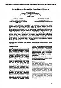
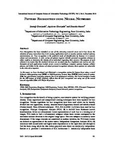
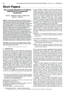
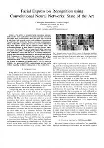
necessary, and are often accelerated by the deliberate omission of some letters from the word being spelled. A common assumption of people unfamiliar with Deaf culture is that a single international sign language is used by all signers. In fact the manual languages are even more fragmented than vocal languages, with distinctly different sign languages being used in countries with the same spoken language. For example, English is the primary spoken language in Australia, the United Kingdom and the United States of America but three independent sign languages are in common use in these countries (Auslan, British Sign Language (BSL) and American Sign Language (ASL) respectively).2 As well as using different signs, different sign languages will often use alternative manual alphabets as well. For example the manual alphabet used in conjunction with ASL involves only a single hand, whereas the fingerspelling system used in Australia is two-handed. These two alphabets are illustrated in Figures 2.1 and 2.2. Even within a single country it is quite common for two or more manual languages to be in use. For example in Australia both Auslan and Signed English (SE) may be used. These languages are representatives of two different approaches to manual communication, and the distinction between them is of some interest when developing an automated sign recognition system. Signed English is a manual representation of the English language. Each sign in SE corresponds to an English word, and standard English grammar is used. Hence SE has basically the same relationship to spoken English as does written English – it is a different representation of the same language.
2It
is speculated that this diversity can be partially accounted for by the lack of long-distance communications devices for the deaf, and the limited media portrayal of sign language. It would appear that for vocal languages media influences such as television and movies may help to reduce geographical variations in language.
9
Figure 2.1 The American manual alphabet (source: Christopher 1976) 10
Figure 2.2 The Australian manual alphabet (source: Johnston 1989b) 11
Auslan, on the other hand, is a specifically manual language, adapted to the special requirements of manual communication, as are its international equivalents like BSL and ASL. Its grammar is distinctly different from that of English or any other vocal language, as it has arisen from the differing constraints and possibilities offered by manual communication. One of the most interesting variations is the use made of spatial aspects of signs to convey grammatical concepts such as tense. An in-depth discussion of Auslan grammar would be too extensive to include in this thesis; for more information see Johnston (1989a, 1991) As a manual language Auslan is more efficient than Signed English. The average signer can produce signs at roughly half the rate of standard speech. However due to its grammatical structure Auslan signers can communicate at a rate roughly equivalent to speech. Signed English by comparison retains standard English grammar and therefore is slower than both spoken English and Auslan. SE has been developed and used primarily because it was felt that it would improve the English language skills of deaf people. The choice of which language should be taught to deaf children is controversial, and is not addressed in this project. Moscovitz and Walton (1990) provide an extremely readable discussion of this issue. For the purposes of developing SLARTI it was decided to concentrate on signs from Auslan. It was hoped that such a decision would make it easier to obtain help from members of the Deaf community during system development, and also aid acceptance of the final system. In addition the Auslan courses run by the Tasmanian Deaf Society and the Auslan Dictionary compiled by Trevor Johnston (1989b) greatly helped in acquiring the background for developing an Auslan-based system, whilst similar resources for SE were not as readily available. It should be noted that all illustrations of Auslan signs used in this thesis are drawn from this dictionary, and I am extremely grateful to Dr Johnston and his illustrator Peter Wilkin for their work in creating such a valuable reference. Unless otherwise specified all of the examples of signs given in this thesis are drawn from Auslan.
2.2 Structural components of signs Although primarily a manual language, signing also relies on non-manual features such as facial expression and body language to provide some of the subtle nuances which make human communication so expressive. Facial actions such as raising of the eyebrows, smiling or puffing out the cheeks can 12
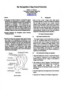
modify the meaning of the sign being performed, in much the same manner that variations in the voice or use of coverbal gestures alter the meaning of words being spoken. Interpretation of subtle variations such as these was felt to be beyond the scope of this project, and therefore only the manual components of signing will be considered in this thesis. Individual signs may involve the use of one or both hands. If only one hand is required, the same hand will consistently be used by a particular signer and this is referred to as their dominant hand. The majority of signers are right-hand dominant and therefore all illustrations and examples used in this thesis will also use the right hand. Similarly the choice of sensing device used for this research restricts the SLARTI system to recognition of signs performed by right-handed signers. However the system could easily be adapted to a left-handed user if the appropriate sensing technology was available by the addition of some simple pre-processing of the input data prior to passing that data to the SLARTI system.3 A study analysing ASL reveals that 40% of signs use a single hand, 35% have both hands active and 25% have the subordinate hand serving as a base for the action of the dominant hand. Of the signs with both hands active, the majority involve both hands making the same motion, either simultaneously or in opposing directions (Klima and Bellugi, 1979). An examination of the Auslan dictionary indicates that similar ratios hold true for Auslan. The signs depicted in Figure 2.3 illustrate the possible combinations of one and two hands that may be used in signing. Water uses only a single hand. Upward demonstrates both hands performing the same action, whilst shelf illustrates the hands making symmetrically-opposite movements. In iceskating both hands perform the same motion, but at alternating times. In bully the subordinate (left) hand serves as a base for the dominant (right) hand. Analysis of individual signs indicates that their manual component can be described in terms of four features – the handshape, orientation, place of articulation and motion (Johnston, 1989b)
3There
would be no need to modify the glove data in any way, but the data measuring hand location and orientation would need pre-processing to reflect the fact that the directions 'left' and 'right' are reversed due to the change in the signer's dominant hand.
13
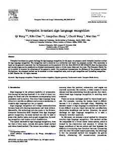
Figure 2.3 Example Auslan signs; top row (left to right) – 'water', 'upward', 'shelf'; bottom row – 'ice-skating', 'bully' (source: Johnston 1989b) Handshape refers to the position of the joints of the fingers and wrist. Each sign language uses its own distinct set of handshapes, although the physical structure of the hand means that the majority of handshapes are common to most languages. Orientation is the angle of the hand with respect to some fixed plane. Generally the different orientation possibilities are described by defining the relationship between the signer's hand, and the body (eg weigh has the palm facing upwards and fingers pointing away from the body). The place of articulation (or location) of a sign refers to its spatial location with respect to the signer's body. Signs can be made on or near particular parts of the body, or in the space in front of the chest which is referred to as 'neutral space'. Motion is the most complex aspect of a sign to describe, as it can consist of variation over time in any of the other three aspects. A sign may involve a transition from one handshape to another (eg ten), or wiggling of the fingers while maintaining the same basic handshape (eg piano). The orientation may change either through a single twisting of the wrist (eg air) or through repeated twisting (eg helicopter). Movement from one place of articulation to another, or through neutral space is a common component of signs (eg elephant). Signs may also incorporate more than one of these motions (eg the sign for involves a change in both handshape and orientation). 14
Figure 2.4 Example Auslan signs; top row (left to right) – 'weigh', 'ten', 'piano', 'air'; bottom row – 'helicopter', 'elephant', 'for' (source: Johnston 1989b)
2.3 Components of Auslan signs 2.3.1 Auslan handshapes Johnston (1989b) analysed the structural component of Auslan signs in developing a dictionary of the language. Within this dictionary signs are grouped initially by the handshape of the dominant hand, and then by the other features (orientation, place of articulation and motion). Auslan distinguishes between 31 basic handshapes. Some of these handshapes may have alternative formations which are not important variations for distinguishing between signs. Johnston identifies 32 of these variant handshapes. All 63 handshapes are illustrated in Figure 2.5, which also includes Johnston's names for each shape which will be used within this thesis. Closer examination of this illustration will yield the observation that two handshapes are repeated within those identified by Johnston. The basic four handshape is also treated as a variant formation of the spread hand. Similarly the second variant of the hook handshape is identical to the second variant of the gun handshape. For the purposes of SLARTI it was necessary to eliminate one member of each of these ambiguous pairs of handshapes. In the first case the decision was simple – the four handshape is used in only one sign (the number four) and hence was eliminated in favour of the more commonly used spread variant. In the second case there was little to recommend one use 15
of the handshape over the other, so the hook variant was arbitrarily chosen to be retained. Eliminating these handshapes does not restrict the number of signs which can be recognised by SLARTI. Signs based on the discarded handshapes can be treated as using the version of that shape which has been retained. Therefore SLARTI is based on 30 basic handshapes, with a further 31 variant handshapes.
Figure 2.5 The primary and variant handshapes used in Auslan (source: Johnston 1989b) 16
Table 2.1 Relative frequency of use of handshapes in the Auslan dictionary Handshape
Number of signs
% of total
Flat
731
20.2
Point
463
12.8
Spread
372
10.3
Fist
372
10.3
Good
139
3.8
Spoon
191
5.3
Hook
164
4.5
Gun
166
4.6
Round
133
3.7
Cup
140
3.9
Two
137
3.8
Okay
129
3.6
Middle
70
1.9
Bad
55
1.5
Three
38
1.1
Ambivalent
48
1.3
Write
61
1.7
Eight
24
0.7
Salt
23
0.6
Rude
8
0.2
Wish
42
1.2
Mother
57
1.6
Perth
33
0.9
Animal
5
0.1
Letter-n
3
0.1
Queer
2
0.1
Letter-m
1
0.0
Four
1
0.0
Seven
1
0.0
Nine
1
0.0
Ten
1
0.0
Total
3611
17
It should be noted that these handshapes are used with widely differing relative frequencies in Auslan, in much the same way that some letters are far more commonly used than others in written English. The division of the signs in the Auslan dictionary by handshape allows the calculation of the figures in Table 2.1 which measure the relative frequency of use of each of the 31 basic handshapes within the Auslan dictionary. From this table it can be seen that the four most commonly used handshapes (flat, point, spread and fist) account for more than half of the signs in the dictionary. This dominance is explained by the fact that these are the easiest handshapes to produce and to visually distinguish from one another. 2.3.3 Auslan hand orientations The orientation of the hand can be described by two values – the direction in which the palm is facing and the direction in which the hand is pointing. When the hand is in a configuration which involves bending the fingers, the direction used is that of the hand as a whole rather than the fingers. This ensures that the description of the orientation of the hand is independent of the handshape. The majority of signs involve orientations which can be described in terms of the six primary directions for the palm and the hand (left, right, up, down, towards the body, away from the body). A smaller number of signs exist in which the hand is orientated diagonally between these main directions. However such minor variations are not easily detected visually, and hence are not used as the sole differentiating properties between pairs of signs. Hence the SLARTI system considers only orientations aligned with the primary directions. Given this restriction it would appear that there are 36 possible distinct hand orientations. However two factors act to limit this number. First, the palm and hand directions must be orthogonal to each other, meaning that for each palm orientation there are only four possible primary hand-directions. Second, certain combinations of palm and hand orientation are extremely difficult to produce due to the mechanics of the shoulder, elbow and wrist joints and therefore are not used whilst signing. For example, the combination of palm facing away from the body and hand pointing downwards is extremely difficult to make (it can be made with the hand below the waist but signs are almost exclusively performed above the waist). Table 2.2 is based on an analysis of the signs in the Auslan dictionary and summarises the 15 orientations which are most commonly used in Auslan.
18
Table 2.2 The 15 most commonly used hand orientations in Auslan Palm direction
Hand directions
away
left, up
towards
left, up, down
up
left, away, towards
down
left, away
left
up, away
right
away, towards, down
2.3.3 Auslan hand locations The location of Auslan signs can be divided into three groups – neutral space, primary locations (those on or near the body) and secondary locations (on or near the hands). Secondary locations are only used in two-handed and double-handed signs. The primary locations can be subdivided into eighteen different places of articulation, which are illustrated in Figure 2.6.
Figure 2.6 The primary places of articulation in Auslan (source: Johnston 1989b) 2.3.4 Auslan hand motions Motion is the most difficult component of signing to analyse, as so many variations exist. Klima and Bellugi (1979) describe Stokoe's attempt to classify the movements used in signing. Whilst this taxonomy was developed in relation to ASL, a similar range of movements are also used in Auslan. Stokoe identified five major categories of movement, which are listed in Table 2.3. Many possible movements can be made within each of these categories (particularly within the directional movement), and signs may consist of a combination of movements performed either sequentially or simultaneously. 19
Table 2.3 The basic movement categories identified by Stokoe Movement type
Description
Hand-internal
Fingers can be wiggled, bent, opened or closed
Wrist
Supinating, pronating, nodding or rotating of the wrist
Directional
Moving the hand along paths in space, generally along the orthogonal planes in neutral space
Circular
The hand can be moved in circles by moving the shoulder, elbow or wrist
Interaction
The two hands can interact, moving towards each other, grasping each other or interlocking fingers
These movements can be further grouped into two general categories – large scale motions which involve the spatial relocation of the entire hand, and small scale motions which involve movement of finger or wrist joints. For the purposes of this thesis motions which involve changes in the hand's location will be referred to as trajectories, in order to distinguish them from the motions involving changes in orientation or finger/wrist positioning. In the absence of a definitive list of the motions used in Auslan, SLARTI is based on an analysis of the motions used in the signs selected for its vocabulary. This process is described in more detail in Chapter 10.
20
3 Hand-sensing technology In computer recognition of spoken language, speech data is captured using a microphone connected to an analog-to-digital converter. Similarly, a datacapturing device is required in order to recognise sign language; in this case measuring the position and movement of the signer's hands. Until recently such technology did not exist, but the growing interest in virtual reality has lead to the development of sensing systems for measuring the movements of the human body, and in particular the human hand. There are two separate sets of values which need to be measured for sign language recognition (and also for many virtual-reality applications). The first is the flexion of the individual joints of the fingers and wrist which define the posture of the hand. The second is the spatial positioning and orientation of the hand as a whole. In general different technologies have been used to measure these two sets of attributes.
3.1 Measuring joint positioning 3.1.1 Instrumented gloves Along with the head-mounted display, the instrumented glove has become the publicly recognised face of virtual reality. The majority of media articles on VR feature one of these two devices, and books such as Rheingold (1991) and Aukstakalnis and Blatner (1993) feature a glove prominently in their cover artwork. It is interesting, given this close connection between VR and instrumented gloves, that such devices generally were not originally developed for use in VR. "Sayre" glove Although research had been conducted into heavy exoskeletons which strapped onto the hand as far back as the 1950s, the first of the modern lightweight hand-measuring devices was probably that developed by DeFanti and Sandin (1977). Their glove was based on an idea by Rich Sayre from the University of Chicago, and consisted of flexible light-conducting tubes mounted along the fingers of a glove with a light source at one end of the tube and a photocell at the other. The amount of light reaching each photocell was reduced as the corresponding finger was flexed, and the resultant changes in voltage produced by the photocells could be monitored to measure the bend of the finger (Sturman 1992).
21
Digital Data Entry Glove Another early glove was that patented by Gary J. Grimes in 1983. Grimes designed a glove capable of converting hand positions into alpha-numeric characters. This glove used a wide variety of different sensors to measure the flex of finger and wrist joints, and also to detect contact between various parts of the hand such as finger tips. These sensors were positioned specifically to recognise the handshapes used in the single-handed manual alphabet, and hence this glove could not be used as a general-purpose handmeasurement device (Grimes 1983, Sturman 1992, Bevan 1995). VPL DataGlove Grimes' employer, Bell Telephone Laboratories, did not develop his glove further however, and so the first commercially produced instrumented glove was the DataGlove manufactured by VPL. This product arose out of the desire of Thomas Zimmerman to use his hand to control a musical instrument without touching it – in effect to actually play 'air guitar'. Zimmerman's initial prototype was built out of an old work glove and several flexible hollow tubes which conducted light. These tubes were coupled with a light source and photosensor and used to measure finger flexion in the same manner as in DeFanti and Sandin's earlier glove. Zimmerman patented this device in 1982, and later went on to found VPL along with VR guru Jaron Lanier. VPL's researchers developed Zimmerman's early glove into the commercial version of the DataGlove, replacing the lightconducting tubes with more accurate bundles of fibre-optic cables. These cables were treated by being carefully scored or cut. As a finger and its corresponding cable are bent, the gaps formed by these cuts becomes larger, and therefore more light is lost from the cable and fails to reach the photosensor. PowerGlove In 1989 Mattell began marketing the PowerGlove as an interface device for Nintendo game systems. Jointly developed by VPL and Abrams-Gentile Entertainment, this device offered hand-measuring capabilities at a greatly reduced cost (around 1/100 the cost of the DataGlove). The glove itself was manufactured from heavy-duty plastic and the expensive fibre-optic sensors were replaced by strips of plastic coated in electrically conductive ink. The resistance offered by these strips alters as the fingers are bent. The cost reduction came at the expense of vastly lower performance – the PowerGlove measures only the overall flex of the thumb, index, middle and ring fingers 22
with only two bits per measurement. This makes the PowerGlove too limited for high-end applications, but its affordability has made it extremely popular amongst 'home-brew' virtual reality developers. CyberGlove The CyberGlove was developed by Jim Kramer at Stanford University as part of his research into sign-language recognition (the recognition aspect of Kramer's work is discussed in Chapter 4). Kramer found that the DataGlove was not sufficiently accurate for his needs, and initially developed the CyberGlove for his own use. It is now produced commercially by Virtual Technologies. The major difference between the CyberGlove and the other gloves already described lies in the sensing technology used. The sensors in the CyberGlove consist of two flexible strain gauges mounted back to back. A pair of gauges is sewn into the glove over each joint to be measured and wired in a Wheatstone bridge configuration. The resistance of the gauges varies as they are bent and by sampling this variation the angle of the corresponding joint can be calculated. The advantage of this style of sensor over the fibre-optic approach used in the DataGlove is that the variation in response of the strain gauges is linear over the entire angular range, whilst the DataGlove sensors have non-linear variation. This makes the CyberGlove's sensors more consistently accurate (Kramer and Leifer 1987, Virtual Technologies 1992). The 5th Glove The 5th Glove was developed by Fifth Dimension Technologies and was released in the United States in May 1995 by General Reality Company. Exact details of the gloves specification are unclear at time of writing, but it appears to be based on a fibre-optic sensing system similar to that used by the DataGlove. From the values quoted for sensor update rate (125 Hz) and complete-hand update rate (25 Hz) it can be calculated that the 5th Glove provides only a single sensor per finger (similar to the PowerGlove). However the sensing technology used is considerably more accurate than that of the PowerGlove. The most interesting aspect of this glove is that at a cost of around US$500 it fills a gap in the market between the low cost and low performance of the
23
PowerGlove and the high cost, high performance option of the DataGlove or CyberGlove (General Reality Company 1995). Dextrous HandMaster Although it is worn over the hand, the Dextrous HandMaster (DHM) produced by Exos differs from the other devices described in that it consists of an exoskeleton rather than a glove. The exoskeleton is held to the user's hand by velcro straps. Each joint of the exoskeleton is equipped with a Hall effect sensor. This sensor is based on altering the magnetic field surrounding a semiconductor as the joint bends, which affects the voltage output by the semiconductor. Due to the precise mechanical linkages between the movements of the hand and exoskeleton joints and the accuracy of the Hall effect sensors, the DHM provides a much higher level of precision than any of the other hand-sensing devices discussed previously. Error rates in the region of 0.5°-1° are attainable. As a disadvantage however this system is bulky and heavy when compared to glove-based devices. For these reasons the main applications of the DHM have been for robotic control systems, where an extremely high level of precision is required. 3.1.2 Camera based joint measurement An alternative approach to specialised glove-based hardware is to use standard video camera equipment to capture a visual image of the user, and then make use of computer vision techniques to extract data about the hands from this image. This avoids the expense of using special purpose handmeasuring devices, but introduces other problems due to its indirect nature. Primary amongst these difficulties is locating the position of the hand and fingers within the image. The hand can usually be located relatively easily, particularly if user's clothing and the background are chosen so as to contrast with the colour of the hands. Extracting the position of individual fingers from within the image of the hand is a much more difficult task, as in many hand positions the fingers will be occluded by each other and by other parts of the hand. In addition the lack of colour contrast between the fingers and hand makes the digits difficult to locate even when they are fully visible. The most common response to these problems is to place artificial markers on the points of interest on the hand (usually the fingertips and the joints of the fingers). Placing multiple markers at different angles on the hand can partially help to overcome problems of occlusion. 24
Sturman (1992) states that LEDs were commonly placed as markers on the hands, body or limbs of subjects in biomechanical research during the 1980s. The light emitted from these devices makes pin-pointing them in the camera image easier, particularly if filmed against a dark background. Other researchers such as Holden (1993, 1995) and Dorner (1994) have used specially coloured gloves worn by the user to aid in this feature extraction process. Their work is discussed in more detail in Chapter 4. Once the hand markers have been identified in the video image, it is necessary to convert this raw data into a more readily useful format, such as finger-joint angles. This can be done by matching the visual-position data against a model of the hand and calculating the required values from this model. Again this process is covered in more detail in Chapter 4. Myron Kreuger (1990) has developed several non-immersive virtual reality systems, which rely on extracting data about the user from a video image.4 Kreuger's systems convert the user's image into a silhouette and then gather data about their motions from this silhouette. Whilst some hand gestures are recognised, this is possible only if they are made away from the body so as to be visible in the silhouette. Therefore this technology is not suitable for gathering sign-language data, in which the hands are often placed on or directly in front of the body. Research being conducted at Bielefeld University is also attempting to bypass the use of markings on the hands by classifying hand postures directly from a video image by using Local Linear Mapping (LLM) neural networks. So far this research has been based on simulated images generated from a computer model of the mechanics of a human hand. The LLM network is trained on images of hand postures presented at various orientations and learns to classify these postures. When applied to images of real hands the results have been promising although still well short of the accuracy required for this approach to be practical for recognition of real hand gestures (Meyering and Ritter 1992a, Meyering and Ritter 1992b).
4
Non-immersive is a term used by some virtual reality researchers to describe systems which do not require the user to wear hardware, as opposed to immersive systems which are based on devices such as instrumented gloves and head-mounted displays.
25
3.2 Position tracking The devices described above only capture part of the information required for gesture recognition. In addition to the information on finger position it is also necessary to track the spatial position and orientation of the user's hands. Similarly, many VR systems require tracking of these aspects for both the hands and head of the user. As a result several alternative technologies have been developed for tracking the three-dimensional position and orientation of an object. These tracking systems can be divided into four general categories – mechanical, optical, acoustic and magnetic. Each of these technologies has different benefits and disadvantages, and as yet none has established a position of dominance within the VR community (Meyer et al 1992). 3.2.1 Mechanical systems Mechanical tracking devices operate by physically linking the object being tracked (which will be called the subject) to a reference point. To provide mobility of the subject the linkages are jointed, and by measuring the angle of these joints the system can calculate the position and orientation of the subject. An early example of this style of system was the 'Sword of Damocles' unit developed by Sutherland in 1968, for use in his experimentation with headmounted displays. This system gained its title from the fact that it was suspended from the ceiling above the user so that it could be attached to the heavy head-mounted display unit. It could track the user through a full 360° of facing, and around 40° of head tilt. Due to its weight the system was uncomfortable for the user, and its main role was to provide accurate data for comparison with a more convenient acoustic tracking system. (Sutherland 1968). More recently Project GROPE at the University of North Carolina used the Argon Mechanical Arm as a tracker for a VR system simulating molecular docking (Brooks et al 1990). Project GROPE demonstrated one of the major benefits of mechanical devices, which is their suitability to systems requiring haptic feedback. The physical link to the user makes implementation of genuine force feedback (as opposed to other haptic systems such as vibration) much easier. Mechanical systems also provide high levels of resolution and accuracy. 26
The major disadvantages of mechanical devices are the limitations they impose on the user. The need to maintain a physical link to the user means such systems cannot provide full freedom of movement to the user, as the linkages can block certain movements. 3.2.2 Optical systems A number of different approaches can be taken to the development of optical tracking systems. They vary in using either ambient light or dedicated light emitters, and in the number and type of sensors used. The most common style of optical position tracker is the fixed transducer system which is based on having either emitters or sensors fixed at a known distance from one another. In an 'inside-out' system the sensors are mounted on the subject and look out at emitters which are fixed to the walls and/or ceiling of the room containing the system. In an ''outside-in' system the emitters are placed on the subject and tracked by fixed sensors. In either system the position of the subject can be calculated by triangulation. Related to these systems are those using pattern recognition. These systems generally use only a single sensor, and therefore cannot use the triangulation techniques employed by fixed transducer systems. Instead the image captured by the sensor is compared to known patterns and the position is calculated from this. Theoretically it would be possible for such systems to work directly from an image of the subject, in the same way as human vision can. However in practice computer vision techniques have not yet developed to this stage and it is necessary to place markers (either light emitters or easily detected patterns) on the subject. A third approach to an optical system is the use of laser ranging. Laser light is beamed onto the subject through a diffraction grating. A camera monitors the diffraction pattern which appears on the subject and can calculate the distance of the subject from the distortion of this pattern. This type of system has the benefit of not requiring the placement of either a sensor or emitter on the subject. However it suffers from ambiguities when the diffraction pattern is projected onto curved surfaces (such as would be involved in tracking a human body), and hence so far has been used mainly for robot vision in more constrained environments. 3.2.3 Acoustic systems Like optical systems, acoustic systems are based on the use of sensors and emitters. In this case, however, the signals used are ultrasonic frequencies in 27
excess of 20kHz, rather than light, and hence such systems are sometimes referred to as ultrasonic position trackers. Two basic styles of acoustic trackers have been developed. The first is a time-of-flight (TOF) tracker, which is based on measuring the time taken for the acoustic signal to travel from the source to the sensor. By using multiple emitters or sensors it is possible to calculate the position of the subject using triangulation techniques (as with fixed transducer optical systems). These systems provide a low sampling rate because of the slow speed of acoustic waves, and the need for the emitter to remain silent for a while after emitting a signal to eliminate possible problems from echoing. They are also prone to interference from ambient noise produced by devices such as cathode-ray tubes. The PowerGlove uses an ultrasonic TOF tracking system. Two ultrasonic transmitters are mounted on the back of the glove and three receivers on a Lshaped frame around the monitor or television which is displaying the output from the Nintendo game unit. The glove must be facing the display unit to work thereby restricting the range of movements which can be tracked. Phase-coherent (PC) trackers work by comparing the phase of a known reference signal to the phase of the emitted signal. Unlike TOF systems the phase can be measured continuously and hence PC systems can generate high sampling rates. This also allows the use of filtering techniques to overcome the effects of ambient noise. However such systems measure only changes in position rather than measuring position directly, and therefore they are prone to accumulation of errors over time. 3.2.4 Magnetic systems Two styles of magnetic position trackers have been developed. The first is based on alternating current (AC) technology and is made by Polhemus, whilst the second uses direct current (DC) technology and is built by Ascension. The Polhemus system is based on a source unit which generates RF magnetic fields, and a sensor which is placed on the subject. Both of these units consist of three orthogonally aligned coils. The emitter's coils are activated to continuously produce three perpendicular magnetic fields. These induce currents in the coils of the source unit which are used to calculate the position and orientation of the sensor. The major problem with this 28
technology is that the continuously fluctuating AC current generates eddy currents in any nearby conductive metal objects. This causes these objects to give off their own magnetic fields, which distort the measurements received from the sensors. To eliminate these errors it is necessary either to remove such objects from the environment, or to fix their location and use software to compensate for their effect on the tracking system. Polhemus has produced several different systems based on this technology. At the time the SLARTI project was commenced the 3Space Isotrak supported a single sensor, whilst the 3Space Tracker could support up to four sensors. These systems have since been replaced by the IsoTrak II (which supports one or two sensors), and the Fastrak (up to 32 sensors). Ascension's DC system operates in a similar manner to the Polhemus trackers, except that the emitter produces a series of pulsed DC fields, instead of continuous AC fields. This reduces the interference produced by eddy currents, as the system can wait for the currents to die down before making any measurements. In contrast the Polhemus' fields continuously generate eddy currents which are still present when the sensor is sampled. In addition the Ascension Flock of Birds can support simultaneous tracking of up to 30 separate sensors. 3.2.5 Comparison of position sensing technologies The different position tracking technologies described above have numerous advantages and disadvantages, which have varying importance depending on the context of the task they are being applied to. This comparison will consider the factors which are relevant to the task of gesture recognition. Due to the direct linkages involved mechanical systems provide extremely high accuracy, but at the cost of constraining the motions of the user. This makes them unsuitable for gesture recognition systems, where the user's hands must be free to move naturally through their complete range of motion. Optical and acoustic systems are more appropriate for this task as they do not constrain the user's motions (as long as the sensors and emitters used are not unduly heavy or bulky). However occlusion of sensors and/or emitters can pose a problem for some systems. Magnetic position trackers are probably the best suited to gesture recognition. Like optical and acoustic systems their interference with the 29
user's movements is limited, and they do not suffer from the occlusion problems of those systems. Conductive and ferro-magnetic surfaces may distort the accuracy of these systems, but this can be overcome by careful choice of the environment in which the tracker is used. Perhaps most important is that such devices have reached a higher state of commercial development and therefore are more readily available than other sensing technologies. For similar reasons these systems are currently the most widely used option within VR systems.
3.3 Sensing technology used for the SLARTI project 3.3.1 Selection of sensing technology The necessary hardware for gesture recognition was not present within the Department of Computer Science when the SLARTI project was commenced, and therefore (within budgetary constraints) it was possible to choose appropriate hardware for the system. The first decision which had to be made was to choose between a camera and a glove as an input device. In one sense this choice was relatively unimportant as the neural networks techniques used within SLARTI could be applied to hand and finger data gathered by any input methods. However as discussed above, extraction of this data from a camera image is itself a complex task. The main research interest of this project lay in the application of neural networks to the recognition of signs rather than extensive imageprocessing, and therefore a glove device was chosen to allow more attention to be focused on the recognition component of the system. 5 Having elected to use a glove it was then necessary to select between the four commercial devices available at the time – the DataGlove, PowerGlove, CyberGlove and Dextrous HandMaster (the 5th Glove was not released until several years after the SLARTI project was commenced). The PowerGlove was immediately eliminated as it lacks the precision and range of sensors required to distinguish reliably between a large number of hand positions.6 The Dextrous HandMaster suffered from almost the opposite problem – in order to provide the high degree of accuracy required for applications such 5
Interestingly, initial indecision over the choice of input technologies was beneficial. The work on missing values discussed in Section 6.3 is primarily inspired by problems foreseen with camera input . Even though this issue did not arise in the final version of SLARTI, this research did result in other ideas which are incorporated into the final system. 6 This decision is supported by the results obtained by Kadous (1995). On the task of recognising handshapes produced by a single user, Kadous reports an accuracy rate of around 94% using a CyberGlove, compared to around 35% using a PowerGlove.
30
as telerobotics (less than 0.5 degrees error) this device is bulkier than is suitable for wearing by a signer (Cochran 1991). The DataGlove and CyberGlove were more viable options, and both fell within the price range available for the project. The CyberGlove was selected over the DataGlove because its strain gauge technology is more accurate and more consistent in a day-to-day setting than the DataGlove's fibre-optics (which are affected by factors such as temperature). 7 The 18 sensor version of the CyberGlove is used for SLARTI, as this includes abduction sensors which are essential for differentiating between some of the handshapes used in Auslan. The requirements of the position tracking equipment were fundamentally those discussed in Section 3.2.5 – no restriction on the movements of the user, and immunity to the problems of occlusion. For this reason magnetic position trackers were the obvious choice. Ideally the chosen system would support multiple sensors for tracking the position of the user's dominant and subordinate hands, and possibly their head. However such systems were not available within the budget of this project. The Polhemus 3Space IsoTrak was the system supplied with both the DataGlove and CyberGlove and therefore it was chosen as the tracking system for SLARTI. This system allows tracking of only a single sensor, which was placed on the user's right hand. The implications of using a single sensor are discussed further in Section 9.3. The two sensing technologies selected for use in SLARTI are discussed in more detail in the following two sections. The current level of research and commercial interest in virtual reality remains high, and it seems reasonable to assume that improvements will be made in both hand-sensing and tracking technology over the next few years. With this in mind the code for SLARTI has been developed in a modular fashion and therefore the techniques used to develop this version should be easily adapted in the future to work with any such improved input devices.
7
Peters (1992) also reports problems with the placement of the abduction sensors on the DataGlove, which pose particular problems for its application to sign language recognition.
31
3.3.2 The CyberGlove The CyberGlove consists of a lightweight cloth glove, with strain gauge sensors and cabling sewn into the cloth along the back of the hand and fingers. The palm and fingertips of the glove have been left open to make it easier to perform actions such as writing or typing whilst wearing the glove, and also to increase the range of hand sizes which the glove will fit. The version of the CyberGlove used in developing SLARTI contains 18 sensors. Earlier versions of the glove provided either 16 or 22 sensors. The major difference between the 18 and 22 sensor CyberGloves is that the latter provides measurements for the outermost joint of each finger (the distal interphalangeal or DIP joint). The positions of these joints are not significant in distinguishing between signs, and in any case can generally be estimated with a fair degree of accuracy from the position of the next closest joint (the PIP). The 18 sensor glove measures the position of the metacarpophalangeal (MCP) and proximal interphalangeal (PIP) joints for each finger, and the MCP and interphalangeal (IP) joints for the thumb. In addition four horseshoe shaped sensors mounted on top of the glove measure the abduction (sideways motion) of the thumb and fingers relative to each other. Finally sensors are also provided to measure pitch and yaw of the wrist and rotation across the palm of both the thumb and the pinkie. This information is summarised in Table 3.1. As well as the joint sensors the CyberGlove also provides a simple binary switch mounted on the wrist of the glove (along with an LED which indicates the state of the switch). During gathering of data for the SLARTI system this switch was initially used to allow the user to indicate when a data sample should be requested from the glove. However the location of the button on the wrist was found to be inconvenient because it required the user's left hand to remain near the right wrist. The switch was also occluded from the user's vision by their hand in certain hand orientations which lead to the user confusing the switch with the Polhemus sensor mounted nearby on the glove. To overcome these problems the glove used for this research was modified so that an external switch held in the user's left hand could be used rather than the glove-mounted switch.
32
Table 3.1 Location and role of the sensors on the CyberGlove Area of hand/glove
Sensors
Thumb
Rotation across palm Metacarpophalangeal angle Interphalangeal angle Abduction (relative to index finger)
Index finger
Metacarpophalangeal angle Proximal interphalangeal angle
Middle finger
Metacarpophalangeal angle Proximal interphalangeal angle Abduction (relative to index finger)
Ring finger
Metacarpophalangeal angle Proximal interphalangeal angle Abduction (relative to middle finger)
Pinkie finger
Rotation across palm Metacarpophalangeal angle Proximal interphalangeal angle Abduction (relative to ring finger)
Wrist
Pitch Yaw
The CyberGlove is connected to an interface unit which amplifies and digitises the values gathered from the glove. This unit can be run in either a continuous sampling mode, or explicitly polled when a data value is required. The maximum sampling rate supported is approximately 30 Hz, and the signals from the sensors are returned as a sequence of 18 bytes giving a resolution of 8 bits per sensor. Within the SLARTI system the CyberGlove interface unit is connected to the serial port of a 486DX PC compatible. Care needs to be taken when using the CyberGlove as the strain gauges in the sensors are fragile. If treated roughly these gauges can become creased which will permanently affect the values produced by the sensor. The abduction sensors are particularly at risk because of their exposed position on top of the glove. For this reason the CyberGlove would not be suitable for use outside of a laboratory environment. 3.3.3 The Polhemus 3Space IsoTrak The Polhemus sensor is attached to the wrist of the CyberGlove, using the built-in mount provided. The sensor is attached by a combination of velcro 33
and plastic screws, as metal screws would cause interference with the magnetic fields used by the Polhemus. The IsoTrak can sample the position and orientation of the sensor up to 60 times per second, which is more than sufficient for the hand movements involved in sign language. The accuracy of the tracker is dependent on the distance of the sensor from the source. Between 4 to 15 inches, the position is accurate to 0.13 of an inch RMS (root mean squared error). From 15 to 30 inches of sensor-source separation the accuracy decreases to 0.25 of an inch RMS. Over this entire range the orientation is accurate to 0.85° RMS. The tracker can be used with separation distances up to 60 inches at lower levels of accuracy. The magnetic fields generated by the source are symmetrical, and therefore there are two possible interpretations of each set of data gathered from the source. For this reason only half of the total sphere surrounding the source can be used at any one time. The hemisphere which is active can be selected by sending an appropriate command to the Polhemus interface unit. In order to avoid errors in the position values returned it is necessary to ensure that the sensor remains in this selected hemisphere. As discussed above, the AC magnetic field technology used by the Polhemus has reduced accuracy as the distance between source and sensor increases, is susceptible to interference from metallic objects and requires the sensor to remain within a selected hemisphere. All three of these problems were observed during early use of the Polhemus and were overcome only by careful positioning of the source with respect to the signer. The IsoTrak source was attached to a plastic base for stability and placed on a wooden table slightly behind the signer at approximately hip height. This kept the system well clear of the ferro-concrete floor of the laboratory. It also placed the source close to the space in which signs would be enacted and hence minimised the distance between the sensor and source. Finally placing the source behind the user ensured the sensor would remain in the chosen hemisphere. Once these issues had been addressed the Polhemus tracker provided sufficient accuracy and reliability for use in this research. However clearly these limitations prevent the current version of SLARTI from being easily portable, and therefore an improved tracking technology would be required in order to develop the system beyond its current prototype stage. 34
4 Hand gesture recognition Dependent as it is on recent developments in hand-measuring technology, the field of hand-gesture recognition is a relatively young one. As a result the majority of the systems described in the literature are only partially completed. The literature is also spread through a wide variety of fields, such as technology for the disabled, pattern recognition, artificial intelligence, human-computer interaction and virtual reality. This section provides an overview of this diverse field, summarising the status of existing research and setting the background for the work carried out on the SLARTI system. It is not intended to be a complete synopsis of all research in the field of hand gesture recognition as the number of researchers in this area has increased dramatically over recent years.8 Instead it focuses on those systems which were of most influence in the creation of SLARTI. Section 4.1 describes systems based on instrumented-glove technology. Due to the same choice of input device these are of the most direct relevance to the SLARTI project. Section 4.2 describes systems based on the alternative technology of image processing. Brief descriptions are given of the image feature extraction methods used, but the focus is on the classification techniques as these could be adapted to other input technologies. Section 4.3 is an overview of the work discussed in the previous two sections, summarising the current state of research in this field and highlighting the issues which have yet to be addressed. Section 4.4 covers the more general area of applications of hand gesture recognition techniques, looking both at existing applications and also potential future developments. For convenient reference to the different projects discussed a simple naming convention has been adopted. Where a system has been named by its authors this name is used. Unnamed systems are referred to by the name of the institution where they were developed, with the addition of some descriptive information about the scope of the project.
8
This rapid growth in the field of hand gesture recognition is largely attributable to the development of instrumented glove technology. The concept even gained enough interest to make an appearance in popular culture – the action film Congo features an ape which uses a sign-language recognition system to communicate with humans.
35
4.1 Glove-based gesture recognition systems 4.1.1 Glove-Talk (Fels and Hinton 1990, Fels and Hinton 1991, Fels and Hinton 1993) The Glove-Talk system is probably the most complete system described in the literature, and its implementation is also the most closely related to that of the SLARTI project. Glove-Talk's gesture system was developed specifically for this project rather than using a pre-existing sign language (although some of the handshapes are based on the ASL alphabet). Unlike natural sign languages there is a well-defined relationship between features of Glove-Talk gestures and the words assigned to them. The handshape made by the user selects a root word from 66 possibilities. An ending for this word is then determined by the motion of the user's hand. Only six motions are legal – a back-and forth movement in any of the six basic directions. The change in direction in this motion is used as the trigger signal to say the word. Each motion corresponds to a different word ending (normal, plural, ed, -ly, -er, -ing). If a word ending cannot be applied to the word indicated by the handshape the normal ending is used by default. Through this method Glove-Talk has a total vocabulary of 203 words. A unique feature of Glove-Talk is that it allows the user to control the manner in which words are spoken by the speech synthesiser. The speed of the user's motion determines the rate at which the word is spoken, whilst the duration of the motion sets the stress which is placed on the word. The gesture recognition component of Glove-Talk is based on five neural networks, the most complex and important of which is the strobe network. This network is responsible for detecting the change in direction of motion, which signals the system to activate the other four networks to analyse the gesture. The strobe network takes 50 inputs consisting of five values for each of the previous ten frames of glove data. These five parameters are the changes in the x, y and z components of the hand's location, the speed of the glove and its acceleration (difference between this speed and the previous one). The network was trained on 596 movement examples in which the strobe point had been labelled by hand (in fact, an early version of the strobe network was used to reduce the workload in labelling this training data by indicating the general region in which the strobe point should lie). By applying a threshold of 0.5 to the network's output an accuracy rate of 97% was achieved on 200 test examples. 36
When the strobe network fires, the glove data is fed into the four other networks. The first of these classifies the handshape as one of the 66 accepted poses. The inputs to this network are the ten finger flexion values, and the sine and cosine of the hand orientation measurements (the sine and cosine are used to eliminate discontinuities in the orientation data – this problem is discussed in detail in Chapter 6.4). This network achieved around 98% accuracy on a test set of 2178 examples. The word-ending network takes as input the changes in the x, y and z position for the previous ten glove measurements and classifies the motion as one of six classes. Not surprisingly, given the simple motions used, it achieves in excess of 99% accuracy on a test set of 499 examples. The word speed and stress networks both take the previous twenty frames of glove speed and acceleration as input. The speed net has eight outputs which are combined to yield a speaking rate of 130 to 240 words per minute. The stress net has a single output which determines the emphasis placed on the spoken word. The performance of these nets is not as vital as for the other nets, but both achieve acceptable results, although the speed net was found to be somewhat dependent on the gesture being performed. When the networks are combined, the overall performance of the system is very promising. Around 94% of gestures result in the correct word being spoken, 5% in no word being spoken and only 1% in the wrong word being produced (as this is the most disruptive form of error it is important that this type of error be minimised). 4.1.2 Glove-TalkII (Fels and Hinton 1995a, Fels and Hinton 1995b) Although sharing the same name, authors and much of the same technology as the Glove-Talk system, Glove-TalkII takes a fundamentally different approach to the mapping of hand gestures to speech. The original Glove-Talk maps each gesture to a single word. Glove-TalkII is based on a much finer grained approach in which features of the hand are mapped onto the articulatory features which control the production of speech. In this way the user can determine properties of the speech such as pitch and volume to produce more natural speech than would result from direct text-to-speech synthesis.
37
In order to provide this greater degree of control over speech parameters Glove-TalkII uses a wider range of input devices. In addition to the CyberGlove and Polhemus tracking system used in Glove-Talk, this system requires a foot pedal and a Contact-Glove (a glove equipped with switches to measure nine different contact points between the thumb and fingers of the left hand). Glove-TalkII uses a combination of several neural networks and several fixed mappings to convert the values from these input devices into the controlling parameters for a parallel formant speech synthesiser. The three neural networks in the system map the user's right hand formation and position onto consonant and vowel phonemes. Separate networks are trained for vowels and consonants, to map the input hand data onto the synthesiser parameters to produce the corresponding phoneme. Vowels are distinguished by an open hand shape (no contact between the thumb and fingers), and the choice of vowel phoneme is determined by the spatial location of the hand in a horizontal plane in front of the user. Consonants are represented by closed hand positions, with each different consonant phoneme corresponding to a different handshape. In addition the switches on the Contact-Glove worn on the left hand are used to select stop consonants as it was found that these phonemes required faster variation of the synthesiser parameters than could be readily controlled by the user. A third network is trained to distinguish whether the user is trying to make a vowel or consonant sound depending on the openness of their hand. The output of this network is used to combine the outputs of the vowel and consonant networks to produce the parameters passed to the synthesiser. The pitch of the speech produced is determined by a fixed mapping based on the height of the user's right hand, whilst the position of the foot pedal controls the volume of the speech. Hence to produce a word the user makes the handshape corresponding to the starting phoneme and depresses the pedal to start the sound from the synthesiser. They then move their right hand through a continuous gesture varying in location and handshape to produce the sequence of phonemes (and appropriate pitches) which form that word, using the contact switches on the left hand to make stop consonants if any are required. In this manner Glove-TalkII can produce any word which can be made up of the phonemes provided and hence does not limit the vocabulary of its user. A demonstration of communication using Glove-TalkII is available on video tape, which shows a user speaking, carrying on a conversation and even 38
singing (Fels and Hinton 1995a). From this demonstration it is clear that the system does allow the production of speech which is more intelligible and emotive than that produced by direct text-to-speech synthesis. However learning to use the system is a non-trivial task (the user shown on the tape was a trained pianist with approximately 100 hours of practice with GloveTalkII) and requires the user to be able to hear the speech being produced. Hence this system is best suited to speech impaired individuals with unimpaired hearing as it essentially turns the hand into an artificial vocal tract. 4.1.3 The Talking Glove (Kramer and Leifer 1987, Kramer and Leifer 1989) The Talking Glove system developed at Stanford University is the project which gave rise to the creation of the CyberGlove, as discussed in Chapter 3.1. The overall aim of this project is the creation of a portable two-way communication system between nonvocal deaf individuals and hearing individuals. To provide two-way communication this system uses a variety of input and output devices. The CyberGlove captures hand data from the signer, and converts this into text which can the be turned into audible speech by a speech synthesiser unit. In the final system it is foreseen that this speech would be emitted through a small speaker on the signer's lapel. Input from the non-signer would be either from a voice recognition unit or a small portable keypad. Text from this source would then displayed on either an alphanumeric liquid crystal display or a braille display carried by the signer, depending on the quality of their sight. The component of this system of most interest with regards to the SLARTI project is the implementation of fingerspelling recognition. The Talking Glove is capable of taking the hand data from the CyberGlove and interpreting these handshapes as letters from the American manual alphabet. Only finger and wrist joint information is used, as the Talking Glove was not equipped with any form of position tracking.9
9
Within the American manual alphabet there exists two pairs of letters ('I' and 'J', and 'D' and 'Z') which use basically identical handshapes and are distinguishable only by motion. Although it would seem difficult to classify between these pairs of letters without use of a position tracker, it was observed during early development of SLARTI's handshape network that the pairs could in fact be distinguished on the basis of wrist position, although this is not a distinguishing characteristic used by human signers (the wrist is flexed in both 'D' and
39
Two different approaches to recognition of handshapes are described in the papers by Kramer and Leifer. In the earlier version each of the sensor values is treated as one component in an overall hand-state vector. Letters are represented as 'beacons' in this hand-space. When the algorithm detects a reduced hand-state velocity (ie a more static hand formation) the nearest beacon to the current state is determined and if this distance is beneath a certain threshold then the corresponding letter is output. To avoid unwanted repetition of the same letter it is required that the hand-state leave this recognition hyper-sphere around each beacon and re-enter it in order to repeat a letter. Special, non-standard fingerspelling states exist to denote backspacing and the end of a word (this signal tells the system to send the completed word to the speech synthesiser). After a word has been spoken the letter beacons are updated to adapt to variations in the formation of letters and the placement of sensors. Kramer and Leifer propose that the recognition rate of the system could be improved by weighting the axes of hand-space to achieve maximal separation between the letter beacons (Kramer and Leifer 1987) This suggestion of using a weighted space is very similar to the neural networks approach, and in fact the recognition method described in Kramer and Leifer (1989) is based on neural networks. In this system a pre-trained neural network is used to select the most probable letter from a dictionary of previously stored hand formations which are individualised to a particular user. The dictionary evolves during use to account for the variations in letter formation between users, although the exact details of this adaptation are not described. As before once the end of a word is signalled by the user the entire word is output to the speech synthesiser. The authors proposed future development of the system to include a position tracker so that the gesture recognition capabilities could be extended to recognise signs from Pidgin English. Another goal was reduction of the size of the system to make it truly portable. The major obstacle to be overcome in this process was implementing the recognition algorithm in a portable unit, rather than sending the glove data to a personal computer. In September 1995 Virtual Technologies (the company founded by Kramer to market the CyberGlove) announced the release of its GesturePlus system. 'J', but relatively straight in 'I' and 'Z'). It is speculated that this is the same technique used by the Talking Glove's recognition algorithm.
40
GesturePlus is a hardware device which recognises user-definable gestures measured via the CyberGlove. Due to its commercial nature details of the recognition algorithm used by GesturePlus are not available. However the system does require the user to provide a set of example gestures in order to train the recognition algorithm (Virtual Technologies 1995). 4.1.4 GIVEN (Bohm et al 1992, Vaananen and Bohm 1993) GIVEN (Gesture driven Interactions in Virtual ENvironments) is a testbed for assessing the efficacy of hand gestures as an interface to a virtual reality system. The initial version of GIVEN implements an office environment with a number of objects (desk, teapot and ball) which can be manipulated by the user. User interaction with this environment is entirely through hand gestures, with specific gestures corresponding to actions such as 'fly forward', 'fly backward', 'grab object', 'release object' and 'reset' (return to starting point). The input device used is a VPL DataGlove equipped with a position sensor, although the GIVEN system is designed to be as independent as possible of the input device. To achieve this the system has been split into three separate sections. The Device Driver handles communication with the DataGlove and passes the data obtained to the NeuroGlove module. This module performs the recognition process, and the resultant commands are then sent to the main GIVEN module which implements the virtual office environment. NeuroGlove uses neural networks to recognise both static handshapes and dynamic gestures. The static handshapes (or postures) are recognised by a standard feedforward neural network with a single hidden layer. This network takes ten inputs, corresponding to the DataGlove's measurement of the outer two joints of each finger (the version of the DataGlove being used in GIVEN does not measure finger abduction, rotation of the pinkie or thumb, or wrist flexion). Although exact details of the number of handshapes recognised are not given, it would appear to be at least 20. A pair of tapped delay line networks are used to perform the dynamic gesture recognition (this style of network architecture is described in detail in Chapter 6). The first network takes as input the finger-joint values for each of the last five time-frames, and classifies the sequence as one of ten gestures. If none of the output nodes fires strongly enough to reach a threshold value, 41
this is interpreted as meaning no gesture has taken place and another frame of input is gathered from the glove and propagated through the network. This process is continued until a gesture has been recognised, at which point the results of both this and the second dynamic network are passed to the GIVEN module. The second temporal network is designed to classify the motion of the hand during the gesture. Its input consists of the three values measured by the position sensor on the glove, pre-processed to indicate relative movement (this pre-processing consists of taking the difference between the current position values and those from four time-frames earlier). The network classifies these values into one of seven movement categories. Although the exact nature of these movements is not clear, it would appear they consist of left, right, up, down, towards, away and no movement. The gesture recognition component of GIVEN appears to be in the early stages of development, and the authors' future plans include applying recurrent neural networks to the dynamic gesture recognition component of the system. 4.1.5 NTT/ATR Japanese manual alphabet recognition system (Takahashi and Kishino 1991) The authors describe a simple system for recognition of the 46 Japanese kana manual alphabet gestures. This task is more difficult than that of performing recognition of ASL fingerspelling because of two features of the Japanese system. Firstly, the Japanese manual alphabet includes five gestures which involve movement ('no', 'mo', 'ri', 'wo' and 'nn'), including one which involves a change in handshape ('mo'). The system developed by Takahashi and Kishino considers only the initial handshape involved in each gesture and therefore cannot distinguish between gestures varying only in their movement component. Secondly, because of the greater number of alphabetic components required, not all have a unique handshape and therefore orientation of the hand must be used to differentiate between some gestures. This system uses a VPL DataGlove equipped with ten finger sensors, and also three orientation values from a position/orientation sensor. A user wearing this glove performed each gesture ten times, and these values were averaged to produce a general representation of each handshape. These were then processed to produce a 12-character code for each gesture (10 characters 42
for the finger joints and 2 for the orientation of the hand). Each joint was analysed to see whether it was in a consistent position for each example of a gesture. Joints with a standard deviation over the examples of less than 20 degrees were considered consistent and labelled as either 'H' or 'B' depending on whether they were on average bent less or more than 45°. Joints which exceeded the standard deviation threshold were coded as '-', representing undetermined. Similarly a 2 letter code was determined for orientation representing the direction in which the hand was pointing (up, down, left, right, back, forward) and whether the palm, back or side of the hand was facing outwards. Recognition of new gestures is performed by encoding the measured gesture and then comparing its similarity to each of the 46 predefined codes. When tested this method performs fairly poorly, recognising between 24 and 30 of the gestures correctly on a regular basis. This failure can probably be explained by three factors. First, the system attempts to classify the moving gestures whilst ignoring the temporal component which would make this classification possible. Second, the lack of abduction sensors on the DataGlove means the measured values fail to include some of the features necessary to distinguish between gestures. Third, the classification technique used is extremely crude. The encoding process discards large amounts of information about the gesture and is extremely susceptible to noise because of its use of hard thresholds between classes. 4.1.6 University of Nebraska-Lincoln handshape recognition system (Revesz and Veera 1993) The authors applied a specialised form of neural network known as a matcher neural network (MNN) to the task of classifying static handshapes. The MNN was developed by Revesz (1989, 1990) and differs from the majority of neural architectures in that its inputs, outputs and memory of training patterns are all binary. An input presented to the MNN is compared to the stored patterns using the asymmetric Hamming distance. This distance measure consists of the maximum number of omissions (1s corrupted to 0s) that must occur to either of two binary patterns in order for them to become identical). If one stored pattern is nearer to the input as defined by this distance measure than any other stored pattern then it is given as the output, otherwise all stored patterns of equal distance are combined to produce an output pattern.
43
The raw data from a CyberGlove is pre-processed to convert it to a binary format suitable for a MNN. This is done using an encoding scheme similar to that of Takahashi and Kishino but without the undetermined category: a straight joint is encoded as 0 and a bent joint as 1. A set of feature lists for artificial hand-shapes was constructed, with each shape represented by 17 binary digits (the pinkie rotation sensor on the CyberGlove was not used, thus reducing the number of system inputs to 17). From the 2 17 mathematically possible hand-shapes, those physically impossible to make with a human hand were removed and then a subset of 395 were selected so as to maintain a minimum asymmetric Hamming distance of 2 between each hand-shape. The feature lists of these 395 signs were then presented to the MNN. Revesz and Veera report a success rate of 96% when the MNN was tested on handshapes not seen during its training. However the accuracy of this result must be questioned because apparently only 100 unseen examples were presented to the network, meaning that approximately three of four handshapes were not tested. 4.1.7 Waseda University musical conducting gesture recognition system (Morita et al 1991) This gesture recognition system was developed for the unusual purpose of allowing a human conductor to control a computerised orchestra. Two aspects of the conductor's movements are interpreted by this system – the musical tempo information provided by the trajectory of the baton in the conductor's right hand, and the expressive information conveyed by gestures made by the conductor's left hand. The motion of the baton is captured by a CCD camera. The tip of the baton is equipped with an infra-red light which makes it easy to extract from the resultant image. By tracking the path of the baton tip through a sequence of frames, statistics on trajectory, velocity and acceleration are extracted. These statistics are then used to predict changes in tempo and control the speed at which MIDI instruments are played. Of more interest to this thesis is the part of the system dealing with the left hand gestures. This is based around a VPL DataGlove and a magnetic position sensor. The glove is initially calibrated for a particular user's limits of movement. At each time frame input from the glove is then used to produce a hendectuple of values summarising the hand's current state and 44
recent movement.10 The eleven features considered are shown in Table 4.1. Unlike the two previous systems these input features were real-valued. Gesture recognition is performed by comparing the eleven values describing the user's gesture to a pre-defined table of each of the gestures the system was intended to recognise. Any gesture for which the measure of matching exceeded a certain threshold is considered to have been recognised. Table 4.1 Features used to recognise conducting gestures Vertical position Horizontal position Sum of previous five values of vertical velocity Sum of previous five values of horizontal velocity Sum of previous five absolute values of vertical velocity Sum of previous five absolute values of horizontal velocity Bending of the thumb (first joint + second joint) Bending of the index finger (first joint + second joint) Bending of the middle finger (first joint + second joint) Rotation of the palm Facing of the palm The number of gestures recognised and formal success rate are not given, but anecdotal evidence is presented that a professional conductor unfamiliar with the system was able to successfully use it without any training. The range of gestures recognised appears to be relatively small, which is why the pre-processing is able to discard seven values from the ten provided by the DataGlove. 4.1.8 Fujitsu Japanese sign-language recognition system (Murakami and Taguchi 1991) The system developed by Murakami and Taguchi is similar to that of Takahashi and Kishino in that it considers elements of Japanese sign language. However it is more developed than that system in that it deals with motion-based gestures in addition to static handshapes. Input data is gathered from a DataGlove and position sensor and presented to a pair of neural networks, which have been trained to recognise a set of example signs. The first of these networks is a simple feedforward network, 10
Isn't 'hendectuple' a lovely word? I much prefer it to the Latin-based alternative 'undectuple'.
45
which takes the ten DataGlove finger-joint values and three hand orientation values as input and classifies that hand position as one of 42 shapes used in the Japanese manual alphabet. This network was trained on examples gathered from one group of signers (called the registered group) and tested on handshapes made by a separate group of signers (called the unregistered group). One version of this network trained on only 206 total examples records a 98.0% success rate on handshapes made by the registered signers, but only 77.0% on signs made by unregistered individuals. It is not clear whether the 98% result is on the signs used in training, or on a separate set of signs made by the same people. By increasing the number of training patterns to 252 and training on signs made by six individuals the success rate for the registered signers trained falls to 94.3% but the result for unregistered signers improves dramatically to 92.9%. 252 examples is still a relatively small training set for a problem of this nature and so it would appear likely that further increases in the size of the training set would lead to further improvements in the network's performance. As it is, the neural network approach used in this system clearly outperforms the system developed by Takahashi and Kishino, even ignoring the five moving handshapes which the latter attempted to include. The second neural network was developed to recognise ten Japanese signs for which both handshape and motion are important. The structure of this network is a combination of the Elman recurrent architecture and the input windowed architecture (both of which are described in the section on spatiotemporal neural networks in Chapter 6). The network takes as input the same 13 values used in the first network, and also 18 values which encode the data about hand position. Three absolute position values are taken directly from the position sensor, and used to generate three relative position values (relative to the starting hand position of the gesture being processed by the network). Each of these six values is then converted into three network inputs, by multiplying the value by 0.2, 0.5 and 0.8 (the purpose of this splitting of each value over three input nodes is not elaborated). The network is presented with these 31 input values for the current time-frame and also for the two previous time-frames, giving a total of 93 inputs. In this way the inputs encode some short term memory of the gesture. In addition the network has recurrent links between each of its 150 hidden nodes, which allow it to perform further temporal processing of the input signal. The network was trained using standard backpropagation as with the Simple Recurrent Network, which is discussed in Chapter 6.
46
A separate version of this network was trained for five different signers, rather than attempting to develop a user-independent network as was done for the handshape network. This temporal network is used in conjunction with the original handshape network to classify user signs. Initially data gathered from the glove is presented only to the handshape network and the activation of its output nodes passed through a threshold. When one of the nodes corresponding to a starting handshape of a gesture fires strongly enough to exceed the threshold, the motion recognition component of the system is activated. Subsequent input data is presented to the temporal network and a similar thresholding technique is used to select from amongst its outputs. If the temporal network settles into an unclear pattern of activation the gesture is not recognised by the system. When tested on the five signers used in training the temporal network this system gained 96% accuracy, although again it is unclear whether this was on training examples or a separate test set. Nevertheless this result is encouraging as the ten signs used were deliberately chosen because of their potential for confusion. The modularity of this system and the thresholding technique used to detect the start of signs are similar to the methods used within SLARTI. However the direct encoding of signs in the second network make expansion of this system's vocabulary an arduous task as the entire network has to be retrained. This issue of extending the system's vocabulary is explored further in Chapter 11. 4.1.9 Royal Melbourne Institute of Technology gesture recognition system (Roberts 1994) Roberts' research is based on techniques for statistical classification of gestures developed by Dean Rubine (Rubine 1991a, Rubine 1991b). Rubine's techniques were developed and tested on two-dimensional gestures based on the path of a pen. Roberts' goal was to test whether these techniques were suitable for recognition of three-dimensional hand gestures, specifically those used in sign language. This system is unusual in that it recognises two-handed gestures. This is accomplished by using two gloves, both equipped with Polhemus sensors. The signer's left hand is measured by a DataGlove, whilst the right hand is measured by a CyberGlove. This variation in sensing technology is an accident of the available resources, which fortunately has little impact on the 47
system as the more accurate CyberGlove is worn on the right hand, which is the dominant hand for most signers and therefore provides the most information for recognition purposes. The DataGlove is accurate enough to provide the less detailed information required from the left hand. The recognition component of the system consists of two stages. The first is a feature extractor which processes the raw data of the gesture to extract a vector of descriptive features. Examples of the type of features used are the length of the gesture, the maximum velocity of the hand and the maximum and minimum finger flexion angles. Once this feature vector has been extracted from a gesture, it is passed to a linear classifier. For each possible output class the classifier contains a set of weights, which are multiplied by the input vector to yield a measure of the likelihood of that class being correct. The weights of this classifier are found through training on a set of example gestures, although the training method is not iterative like those used for training neural networks. The exact details of training are discussed in more detail by both Roberts and Rubine, but in essence a mean-feature vector is calculated for each gesture class. These are used to generate an inverse common covariance matrix over all the classes, from which the weights for the classifier can be derived. This system was tested on a dataset consisting of 37 gestures (the 26 letters of the Australian two-handed manual alphabet and the signs for the numbers 0 to 10). 25 examples of each gesture were captured (from a single signer), and these were split into a training set (of 15 examples per gesture) and a separate test set. Due to some errors in the data-capturing sequence some examples needed to be discarded, which resulted in the test set consisting of between 4 and 10 examples of each gesture with a total of 236 examples. Although many of the gestures in fact consist of static handshapes (or 'poses'), all of the examples were captured as gestures over several time-steps to include information about the formation of these static shapes. Several variants of the recogniser were built, varying in the features of the input on which they were based. An initial version based on the feature set designed by Baudel and Beaudoin-Lafon (1993) for three-dimensional gestures performed poorly, achieving only a 16.1% recognition rate on the test set. This result was improved by including features specifically designed to suit the characteristics of sign-language gestures. The best version of the recogniser used the 21 features given in Table 4.2. This system classified
48
94.1% of the test set correctly. The most common error was confusion of the 'i' and 'o' gestures, which are very similar in the two-handed alphabet. The statistical feature extraction and classification techniques employed performed well on the dataset tested. To extend these methods to more complete sign-language gestures it would be necessary to discover features which encapsulate the necessary information about such signs, particularly with regards to the trajectory of hand movements. Two major benefits of this approach in comparison to neural networks are the speed of training of the classifier, and also the ability to add new gestures to the system without extensive re-training. However Roberts suggests that neural networks may prove better able to adapt to the problems of co-articulation, although this conjecture is not tested. Table 4.2 Gesture features used by the most successful version of the RMIT system motion path length gesture duration maximum hand velocity right hand flex for thumb, index, middle and annular fingers (4 values) left hand flex for thumb and index finger (2 values) right hand average spatial position (3 values) left hand average spatial position (3 values) right hand orientation (3 values) left hand orientation (3 values) 4.1.10 GloveTalker (Greenleaf Medical Systems 1991a, 1991b, Greenleaf 1992) GloveTalker is a commercial system and as such only limited information is available about it, particularly with regards to its implementation. It was developed by Greenleaf Medical Systems, a Californian medical technology company headed by Walter J. Greenleaf, and is based on the VPL DataGlove. Greenleaf Medical Systems had exclusive rights to sell the DataGlove to the medical community, and extended this licence to allow them to produce their own DataGloves when VPL's production suffered from quality problems (Hamit 1993). GloveTalker differs from the other systems discussed here in that it does not use a pre-specified set of gestures. Instead it learns to recognise a personalised set of gestures selected by each user, mapping these onto a set 49
of words or phrases which are spoken by a speech synthesiser. This adaptation to the user is particularly useful if the user has limited hand movement. It is also convenient for individuals who have temporarily lost their speech (for example, through throat surgery), as they do not need to learn a complex signing system to use GloveTalker to communicate. Another related Greenleaf product is the Gesture Control System, which translates gestures into operations on a computer rather than into speech. Thus users with limited physical movement (such as those with cerebral palsy) can use this system to perform actions such as answering and routing telephone calls. Greenleaf also developed the Movement Analysis System which uses the DataGlove to measure the range of movement in the hand, for use in assessing the rehabilitation of individuals with hand injuries (Aukstakalnis and Blatner 1992). 4.1.11 University of Milan sign recognition system (Camplani 1992) The original thesis describing this work is in Italian so the details given here are derived instead from a description of the project by Montefusco (1993), and therefore are imprecise about some aspects of the research. The system consists modular construction of several neural networks, and recognised 15 signs from Italian sign language. These signs are described by 22 features (five possible locations, eight orientations and nine handshapes). A single network was trained to take the values provided by a DataGlove and Polhemus and classify static postures in terms of these features. In effect this net consists of three separate classifiers combined together: one for location, one for orientation and one for handshape. A second layer of four networks (one each for handshape, orientation, location and movement) is used to process the temporal aspects of the gestures. Each of these takes as input the last seven activation values of the relevant outputs of the static classifier net. These networks then feed into a final network which has 15 output nodes, corresponding to the 15 signs to be recognised. This network performs the final classification of the gesture. These five networks were not trained in the same manner as standard networks, but had their weights set directly on the basis of a single examination of the training examples. Unfortunately Montefusco does not provide details of this process, nor of the classification rate achieved by this system. 50
4.1.12 MIT Coverbal Gesture Recognition system ( Sparrell 1993, Wexelblat 1994) MIT's Advanced Human Interface Group has conducted a series of research projects aimed at recognition of coverbal gestures (gestures made in conjunction with speech). This research is aimed at the development of intuitive multi-modal computer interfaces capable of accepting input in the form of speech, gesture and eye-tracking. The major difference between coverbal gestures and the gestures studied by other researchers is that in the former case there is no strict mapping between gesture and meaning, or even a defined set of gestures. Instead the user creates gestures as they communicate, and the meaning of these gestures can only be determined in terms of the context of the words spoken as they are made. Wexelblat (1994) describes a feature-based gesture analysis system which has been incorporated within AHIG's demonstration interface. The input devices to this system are a pair of CyberGloves equipped with Ascension Flock of Birds position sensors, and a 'data suit' worn by the user (this consists of a lightweight jacket containing a position sensor and also the cabling for the gloves). The user also wears a head-mounted eye-tracking device and a microphone for voice recognition but these are not of interest for the handgesture analysis process. The raw values from the sensors in these devices are processed by a body modelling algorithm, which calibrates for the user's body size and movement range and converts this data into the angles of body joints such as the elbow and shoulder. These joint angles are then used as input for gesture analysis. The body mapping acts as an interface between the input devices and the gesture analysis system, meaning that the devices can be changed at a later stage without affecting the gesture analysis. The gesture analyser splits the input data sequence into key frames (those involving significant changes in the users position or motion) and extracts a descriptive set of features for that frame. These descriptions of the key frames are then used as input to the AHIG interface interpreter along with the results of the speech recognition component of the system.
51
4.2 Camera-based gesture recognition systems 4.2.1 Sign Motion Understanding (SMU) system (Holden 1993, Holden et al 1994) The SMU system under development by the Robotics and Vision Group at the University of Western Australia uses computer vision techniques to extract hand information from a camera image of the signer. This approach was taken mainly to overcome the fragility of current glove technology, but has the added benefit of being able to consider two-handed signs. When complete SMU is intended to recognise signs from either Auslan or Signed English. In order to facilitate the process of extracting hand data from the video image SMU does in fact require the user to wear a pair of gloves. However these are not instrumented gloves, but thin rubber surgical gloves. By marking the gloves the process of identifying the individual joints of each finger is made much easier than gathering the same information from a user with bare hands. Early experiments with the gloves tried retro-reflective tape and different coloured bands on each joint, but eventually it was found that the best approach was to mark complete portions of the glove in different colours, corresponding to each finger and different sections of the palm. This greatly reduces the problems of identifying fingers which are partially occluded from view by other parts of the hand. Each finger is individually extracted from the image by colour thresholding. Its area is then skeletonised to produce a line, the curvature of which can be analysed to determine the necessary information about finger position. A similar process is applied to the palm regions. The resultant data from a single frame is then encoded into a Static Pose Description (SPD) which contains information on the curvature of the fingers, whether they are spread or closed, the directions of the palms and the relative positioning of the left and right hands. A series of SPDs can then be converted into a Hand Movement Description (HMD) which encodes temporal information such as movement of the fingers (bending, straightening, spreading, closing or crossing over) and movement of the hands.
52
The chosen implementation for SMU's recognition system is a fuzzy expert system. This combines the rule-based knowledge structure of an expert system with fuzzy logic concepts such as partial membership of sets. The expert system takes an HMD as input and uses two groups of fuzzy sets to classify this data. Each static finger position can be classified as straight, slightly bent, greatly bent or completely bent, whilst finger movement, hand motion and wrist rotation are classified as no wiggle, very small wiggle, small wiggle, medium wiggle, large wiggle and very large wiggle depending on the number of velocity changes over the recorded period. As these are fuzzy sets the borders of the sets overlap and so an example can be classified as being a member of more than one set. A characteristic function returns a real value as a measure of the example's possible membership of each set. SMU uses a triangular membership function. Once the fuzzy membership values of the HMD have been calculated, they are passed to the rule-based section of the recogniser. An expert user has generated a rule to describe each sign in the SMU vocabulary. The style of these rules is illustrated by this example from Holden et al 1994 (f0 to f3 are finger measurements; X, Y and Z are the hand motion; Delta is the rotation measure). if
f0 starts as greatly bent, and very small wiggle, ends as straight f1 starts as greatly bent, and very small wiggle, ends as straight f2 starts as greatly bent, and very small wiggle, ends as straight f3 starts as greatly bent, and very small wiggle, ends as straight X does no wiggle Y does no wiggle Z does no wiggle Delta does no wiggle then the sign is 'ten' Although these rules appear binary in nature, this is not in fact the case because of the fuzzy nature of the set membership functions. A rule will fire even if the input values are only possible members of the sets specified in the rule, and the output truth value of the rule will be the weakest membership value of an input variable used in that rule. This output truth value is a measure of the likelihood of that rule being correct for this input. In this manner multiple rules will fire for a given HMD, and the output of these rules is combined to form the final classification.
53
4.2.2 Simon Fraser University ASL translation system (Dorner 1993, Dorner 1994, Dorner and Hagen 1994, Hagen 1993, Hagen and Dahl 1994) Like the SMU system, that being developed by Dorner and Hagen uses a video camera and computer vision techniques to track the user's hands. The user wears a pair of cotton gloves on which the joints and finger tips have been marked with different coloured paint. The markings used are more complex than on the SMU gloves, primarily so that the joints of each finger can be measured independently rather than considering the overall shape of the finger as SMU does. Each joint or fingertip is marked with rings of two colours – one identifying the finger and one the joint type or finger tip. An additional ring of a different colour is used to mark the position of the wrist. Overall this scheme requires the use of ten different colours. An image of the hand is segmented by colour to find the individual markers in a similar manner to SMU. However, because the markers are much smaller than SMU's large blocks of colour, occasionally several possible locations for a particular marker are initially detected. This problem is overcome by a prediction algorithm which attempts to project where the hand and joints will be located on the basis of previous frames. These predictions are generally quite accurate as the hand must obey the laws of inertia, and therefore conflicts can usually be resolved by selecting the potential location closest to the predicted location. In cases where this fails a model of the hand is used to select between the candidate locations on the basis of the physical constraints of the hand. Once all markers have been located the hand model is again used, being adjusted to minimise the error between its two-dimensional projection of joint locations and the actual locations recovered from the image (a Newtonstyle iterative approximation method is used to perform this task). The adjusted model is then used both to determine the measured values of joint bend and hand orientation, and also to predict the state of the hand for the next time frame. Currently this system cannot capture hand information in real time, but may be able to do so with the addition of specialised hardware for detecting the colour markers within the camera image (Dorner 1993, 1994). In the final system the output of this stage would then feed into a signrecognition module. However this second module has yet to be 54
implemented, although the authors suggest that it may consist of two layers. The first would classify each time frame of a gesture in terms of handshape, orientation and location as a form of pre-processing, and these classifications would then be used to determine the motion component and final output of the recognition module. The important difference between this work and the other sign-language recognisers examined is that it intends to go beyond recognising signs to actually understanding the ASL message conveyed by those signs. The sign recognition module would feed into an ASL parser which would extract the semantic content of the sequence of signs made by the user. This parser is based on techniques developed in the field of natural language understanding, and a discussion of its implementation is beyond the scope of this thesis. However such a parser would be an extremely valuable addition to any of the gesture recognition systems discussed, as it would enable the creation of true sign-language to speech translation devices. 4.2.4 University of Central Florida gesture recognition system (Davis and Shah 1993) This system, like SMU and the Simon Fraser University system, is based on extracting hand data from a camera image, and requires the user to wear a specially marked glove to make the image-processing task easier. However Davis and Shah use a glove with only binary markings, rather than the coloured markers used in those projects. This reduces the overhead required in processing the images as binary thresholding can be performed much faster than colour thresholding. The markers are placed on the fingertips of the gloves, and therefore only the position of the fingertips is tracked, rather than the angles of the finger joints. Once the fingertips have been detected in a given frame, a motion correspondence algorithm (developed by Rangarajan and Shah 1991) is used to map the movement of fingertips between the previous and current frames, so that the actual position of each finger can be measured without confusion. At each frame the current position is encoded as a vector of the displacement in position of each fingertip between this frame and the starting position (this discards information about any nonlinear movement of the fingertips). The system allows recognition of eight different gestures as described in Table 4.3. Note that these gestures are similar to those studied by Roberts – the gesture is defined in terms of a static posture, but the system also considers the movement of the hand in forming this posture. The system can 55
recognise a sequence of these gestures, with the restriction that the user must make the 'start' gesture at the start of the sequence and after each gesture. The other seven gestures were chosen for potential use in controlling a robotic arm. These constraints on the user allow the recognition process to be performed using a finite state machine (FSM). States in this machine correspond to the initial start position, the smooth transition of the fingers to the actual gesture, the maintenance of this gesture, and finally the transition back to the start position. The motion of the hand extracted from the image drives the FSM from one state to the next. To reduce the occurrence of premature changes of state a 'three-frame similarity' constraint is imposed, whereby three consecutive frames must exhibit the same type of motion in order to switch the state of the FSM. When the FSM reaches the state associated with the actual gesture having been formed, the current finger displacement vector is passed to the classification algorithm. Table 4.3 Gestures recognised by the University of Central Florida system Gesture name
Gesture description
start
flat palm, all fingers extended
left
ASL letter L – thumb and index finger only extended
right
ASL letter B – start hand but rotated to the right
up
ASL letter G – pointing upwards
down
all fingers curled downwards, thumb extended
rotate
ASL letter Y – thumb and pinkie finger only extended
grab
ASL letter C – all fingers and thumb curled
stop
all fingers closed to the palm, thumb extended
The classifier is based on multiple examples of each gesture, from which the mean direction and magnitude of the displacement of each fingertip are calculated. This displacement vector is stored and also used to generate a gesture code for this particular class of gestures. This 5-bit code is derived by applying a threshold to the mean displacement of each fingertip. When a new gesture is presented for classification its gesture code is calculated, and its displacement vector is then compared to those of any gesture(s) with the same gesture code. Hence the gesture code is used only to reduce the number of comparisons which are required. The gesture is considered to belong to a gesture class if all of its vector fields lie within a certain threshold of the corresponding vector fields of the class. 56
The system performed well in testing, recognising 66 of 70 gestures contained in ten separate sequences. Only one of these errors resulted from an error in the classifier. The other three were due to an incorrect shifting of state in the FSM, which resulted in the classifier being called at the wrong point in the gesture sequence. The major benefit of the FSM method used in this system is its immunity to variations in the speed of a sequence of signs. However in order for this to be possible it was necessary to introduce the artificial reference point of the 'start' gesture between each actual gesture performed by the user. Whilst this may be acceptable for some applications (such as robotic control as discussed by Davis and Shah), this restriction is unsuitable for many other gesturebased applications, in particular sign-language recognition. In addition the simple fingertip tracking used may not be suitable for sign language as it captures only limited information about the hand position and the nature of its movement.
4.3 Comparison and summary of existing systems A large number of sign-language and gesture-recognition systems have been described in the previous two sections. Apart from the obvious variations in both input device and recognition techniques used, these projects also vary widely in the number and type of gestures recognised. Table 4.4 is an attempt to provide an overview of the relative scope and success rates of the systems so far examined. Only those systems for which formal results have been reported are included in this table, and dashes have been used to indicate where the information is not available. Table 4.4 Summary of the scope and accuracy of existing sign language and gesture recognition systems System
Handshapes recognised
Motions Vocabulary recognised size
Accuracy
Glove-Talk
66
6
203
94%
Talking Glove
28
0
28
–
GIVEN
20
7
–
–
NTT/ATR
46
0
46
52-65%
Nebraska-Lincoln
395
0
395
96%
Fujitsu
42
–
10
96%
RMIT
37
0
37
94%
Central Florida
8
0
8
94%
57
Table 4.4 summarises the number of gestures recognised by each system, and the accuracy of their classification. In addition these gestures have been broken down to indicate the number of different handshapes and motions recognised by the system (orientation and location have not been shown as the majority of the systems either do not recognise these features, or do not report the number of possible values classified). For some systems the distinction between handshape and motion is blurred, as they recognise signs defined by static hand positions from temporal hand data (eg the Talking Glove, RMIT). Such gestures have been classified as handshapes to distinguish these systems from those which recognise trajectories of the entire hand. The systems developed so far exhibit three main shortcomings relative to the goal of producing a general sign-language recognition system. First the total number of gestures recognised is relatively small. This limits the potential applications of these systems as their gesture vocabulary is well below that required to act as a fast general communications device (the fingerspelling systems can be used for this type of communication but would be frustratingly slow for anything longer than a few words). In addition the majority of the systems have been developed in a manner which would make extension of their existing vocabularies a time-consuming task. The second common feature is the limited amount of motion involved in the gestures recognised. Most systems either deal only with static handshapes or relatively constrained sets of hand motion (eg the seven motions recognised by GIVEN). In order to handle real sign language the ability to recognise a wider set of motions will be required. The third common failing is that the segmentation of individual signs within a series of continuous signs has yet to be fully addressed. Systems such as Glove-Talk and Central Florida work around this problem by introducing artificial signals between gestures, whilst other systems such as the TalkingGlove and RMIT have started to address this issue within the context of finger spelling. Of the current systems the two versions of Glove-Talk are probably the most developed, recognising a large number of handshapes plus a small set of motions within the context of continuous gesturing (although the specialised motions used by the original Glove-Talk greatly reduce the task of segmenting one gesture from the next). The 395 handshapes recognised by 58
the Nebraska-Lincoln system give it the largest vocabulary of the systems surveyed but it is questionable how many of these can be regularly reproduced by a user, as this is approximately ten times as many handshapes as used by any of the major sign languages.
4.4 Applications of hand gesture recognition The gesture-recognition systems described in this chapter have been inspired by a wide variety of potential applications of this technology. The task of recognising sign-language has been the focus of many researchers, whilst others have been interested in applications such as robotic control. Many of the gesture-recognition techniques developed are not specific to the applications being considered and could readily be adapted to use in a range of applications. This section explores some of the potential applications of hand-gesture recognition, examining both systems already in existence and areas to which these techniques may be applied in the future. 4.4.1 Sign language translation system The creation of systems capable of translating sign language into text or speech is the most ambitious application of hand-gesture recognition technology proposed in the literature. Although this is the goal which has inspired much of the research in this area, the development of practical sign language translation systems is still a long-term proposition as this would require major improvements over current technology. The obstacles facing the creation of translation systems can be divided into three basic categories – the first relating to the hardware used to sense the actions of the signer, the second to the sign recognition algorithms used to process the data gathered by the hardware devices and the third to the translation of the recognised signs into English (or another spoken language).
Requirements for hand-sensing technology Any practical sign language translation system must be portable in order to facilitate widespread use. In addition the system must be robust enough to survive being used in the real world. The field of virtual reality research is still new, and as a result the body sensing technologies on which it is reliant are still better suited to use in closely controlled laboratory environments than in the less predictable (and often harsher) conditions of the real world. The majority of hardware devices discussed in Chapter 3 are not designed for portable use. In some cases this is due primarily to the weight of the devices and their interface units, and also their reliance on external power 59
sources – factors which can be addressed by future developments in the design of these devices. On other cases the lack of portability is due more fundamental features of the device. The various tracking devices are a good example of the latter problem. The optical and acoustic tracking systems require the placement of sensors or sources in the environment around the user, which clearly is infeasible in many real-world situations. Whilst magnetic sensors do not suffer from this problem, they can still be affected by environmental factors such as the presence of metallic objects. In a laboratory setting such interference can be eliminated by careful manipulation of the environment, but clearly this cannot be guaranteed in general. Development of practical, portable sign language translation systems will not be possible until improved sensing technologies are developed (and the costs of such devices have fallen to a more widely affordable level). If the demand for such translation systems were the only driving force it is unlikely that these improvements would take place, as the market for such devices is fairly limited. However it appears likely that many of the hardware improvements described above will be developed within the next few years, as similar problems will be encountered in the development of robust virtual-reality systems and the VR market is sufficiently large to drive such research.11 Requirements of sign recognition algorithms The major requirement of the sign recognition algorithm of a translation system (aside from the high level of accuracy required by all applications of this technology) is the provision of a vocabulary of sufficient size to allow the system to function as a practical communication aid. Ideally the vocabulary of the system should also be extensible, or modifiable to allow the easy incorporation of signs required by a user which are not supported by the default vocabulary. It is also vital for a communications system based on sign language to support finger-spelling, as there will always be occasions when words or names are required which are not in the system's vocabulary
11
The situation bears close resemblance to that of voice recognition technology. The users who benefit most from practical voice recognition systems are probably those with physical impairments. Such technology allows them to use empowering devices such as computers which they may otherwise be unable to access (Esser 1992), and can be incorporated into systems to allow control over other devices and aspects of their environment (SmithKenefick and Jacobson 1992, Noble et al 1993). Such assistive technology would not have existed without the development of speech recognition technology which was driven primarily by the potential commercial and business applications of such technology. Similarly the potentially huge market for VR products will result in the development of devices which can also be applied to creating communication aids for the Deaf.
60
The second major requirement of this type of system is the ability to segment signs so as to recognise the component elements of a continuous sequence of signs. Judging by the experience of speech recognition research it would appear likely that this problem will be a difficult one to overcome – as recently as 1993 commercial speech recognition systems such as Dragon Dictate could not recognise natural speech, requiring a pause of around a quarter of a second between words (Dragon Systems 1993). It may be that similar overheads will need to be imposed on the users of the first sign language translation systems. Translation of sign language to spoken or written language The majority of the work related to automated recognition and translation of sign language has so far focused on the task of recognising individual signs rather than on the consequent process of translating these signs into a spoken or written language such as English. A simplistic approach to the latter task would be to merely pass the English gloss of each sign to a voice synthesis unit, but this would produce poor results due to the major linguistic differences between English and sign languages such as Auslan. In order to produce acceptable results it will be neccesary to develop sophisticated translation systems based on a thorough knowledge of the grammar of the two languages. Automated translators are currently under development for ASL-to-English (Dorner and Hagen 1994) and the inverse translation from English-to-ASL (Lee and Kunii 1992). Whilst some aspects of these systems will be unique to ASL, the general underlying principles should be adaptable to other sign languages. 4.4.2 Sign language training system A less ambitious application, which still aids in breaking down the communications barrier between the Deaf and the general public is the development of a training device for people learning to sign. Generally nonDeaf people learn sign langauge through classes run by groups such as the Tasmanian Deaf Society, usually held on a weekly basis. One of the more difficult aspects of learning a sign language (or a new spoken language) is the inability for the student to be aware of their own errors when practising between classes. The most common approach to this problem is for students to form into pairs or groups to study together, so that each can point out the others' mistakes. Gesture-recognition systems could be adapted to develop an automated study partner to provide similar feedback when human partners are not readily available. 61
This application is less demanding than a full translation system. For example, students will usually only be learning a small vocabulary and initially signs are learnt individually with little reference to the more complex aspects of the language's grammar. Therefore a computer-aided learning system would not require an advanced segmentation algorithm, or knowledge of grammar. Similarly the portability and robustness requirements of a translator are not as essential in this context. A sign language training system would require two basic capacities in order to help the student learn the language – the ability to demonstrate the correct formation of the sign, and then to analyse the student's performance of the sign and highlight any mistakes. Two possible approaches could be taken to illustrating signs. The first is to capture footage of the signs being performed by actual signers. The advent of CD-ROM technology has made the storage and interactive access to large amounts of video a feasible proposition. An ASL dictionary of over 2000 signs is already available on CD-ROM (Sternberg 1995), and another is currently under development at the Boy's Town National Research Hospital (1995). The second approach is to generate computer graphics renditions of the signs from some definition of the signs. The Visual Translation (VT) system developed by Lee and Kunii (1992) takes this approach. The VT system processes natural language text and translates it into sign language which is displayed using three-dimensional animated graphics. This method has the advantage of flexibility in that sequences of signs can be generated 'on the fly', assuming the system contains adequate models of signing behaviour.
4.4.3 Gesture driven interfaces The development of hand-sensing devices has led to the consideration of the hand as a natural input medium for many tasks. Sturman (1992) provides an overview of the possibilities for the use of the hand as an input to interface systems, ranging from controlling multiple MIDI musical instruments to determining the actions of a computer-animated puppet. Sturman distinguishes between interfaces in which features of the hand are mapped continuously onto one or more features of the system being controlled, and those in which discrete positions or motions of the hand are recognised and used as input commands or 'tokens'. The features recognised by the latter 62
may be static hand positions, or more complex gestures, and hence it is this category of interface which will be discussed in this section. Vaananen and Bohm (1993) identify a number of advantages to be derived from the incorporation of gestures into control system interfaces. The most important is the natural mapping of some input tasks onto user gestures, which makes gesture-based interfaces easy to learn and use. Although a natural correspondence between gesture and task does not always exist, making use of such mappings when possible allows the construction of interfaces which use a combination of gesture and other input mode to provide the user with more expressive power. The MIT Media Laboratory has developed a range of systems which demonstrate the capabilities of interfaces combining input paradigms such as speech, gesture and eyetracking (Bolt 1980, Herranz 1992, Thorisson et al 1992) Use of gestures in virtual reality systems One of the areas where hand gestures are already widely used is in VR systems. 'Finger flying' has become a standard means of moving around in glove-based VR systems, whereby the user points in the direction they wish to move and uses the position of their thumb to control the speed of motion. Similarly simple hand configurations are often used as controls for manipulating virtual objects. To pick up an object the user moves their hand until the virtual image of their hand is inside the object, and then forms a fist. The object becomes attached to the virtual hand and will move with it until the user opens their hand (Fisher et al 1986). The GIVEN system (Vaananen and Bohm 1993) uses similar hand gestures to allow the user to control actions such as forward and backward motion, and returning to a starting location in the virtual environment. These examples serve to illustrate the manner in which gestures can be used to produce intuitive interfaces to VR systems. The 'finger flying' and 'pick up' gestures are extremely simple, consisting only of static hand configurations. Gesture recognition systems such as SLARTI offer the potential to incorporate more complex, temporal hand gestures into VR systems, thereby providing the user with a richer interface. One aspect of VR where gestures would be particularly well suited is in allowing the user to rapidly manipulate and modify the virtual objects in the system. VR pioneer Jaron Lanier has stated his desire to create 'usermalleable' systems in which the user can create new virtual objects and environments in a few seconds (Barlow 1990b). The desire for speed requires an expressive interface, which must also be easy to learn and use so as to 63
impose minimal cognitive overheads on the user. A multi-modal interface consisting of voice and gesture would appear a suitable means of implementing such a system. Gestures form a natural means of describing some spatial properties of objects such as their shape, size and motion whilst voice can be used to define other attributes such as colour which are less naturally represented by hand gestures. Use of gestures in robotic control A further area in which gestural interfaces have been explored is the field of robotic control. Remote control of robots either by a user with direct visual contact with the robot or via a teleoperator system, has potential for application to a wide range of tasks which cannot be accomplished by either a human agent or an autonomous robot. Examples include geographical exploration of the surfaces of other planets (McGreevy 1992), and manipulation of objects in a microscopic environment (Robinett 1992). A major issue to be overcome in developing these systems is the need for an interface which provides a natural means for controlling the multiple degrees of freedom possessed by most robotic devices. Sturman (1992) reports that conventional devices such as dials and sliders are often not suitable for controlling more than a small number of parameters, and so more sophisticated interfaces may be required. The use of the hand as an input device (and particularly the use of hand gestures) can provide a more easily learnt and utilised interface. Several studies have been undertaken to examine the manner in which gestures can be used to control robots, based either on actual physical devices or on simulations of such robots. Papper and Gigante (1993) explored the use of gestures to control a simulated robotic arm designed to mimic the structure of the human hand and arm. Hand gestures were used to provide various controls over the robot arm which could not be obtained by a direct mapping from the user's hand to the robot manipulator. For example, parts of the robot could be locked in place, the robot's wrist could be continuously rotated in a manner not possible with a human wrist, and a fine control mode could be entered to allow more precise control over the robot. It was found necessary to include an explicit 'clutch' gesture which toggled the activation of the gesture recognition component of the system, so as to avoid interpretation of unintentional gestures, and to allow the user to reposition their hand. Singh (1993) compared several different mappings for controlling a small robotic arm via a CyberGlove, and reported that a gesture-based control 64
system was easier to learn and operate than systems based on direct mappings from the hand joints to robot joints. This agrees with results reported by Sturman (1992) from experiments based on controlling a simulated crane using a variety of different interfaces.
65
5 Spatial neural networks It is assumed that the majority of readers of this thesis will already be familiar with at least the basic concepts involved in neural networks, and therefore do not require an introduction to the field of connectionism. However it is also envisioned that some readers may lack background knowledge of this area and so this chapter provides a limited introduction to this field, discussing the basic concepts underlying neural networks with a focus on the style of networks used in this research. For a more comprehensive review of neural networks see any of the many textbooks available on the topic – for example Wasserman (1989) or Hertz et al (1991). Section 5.1 provides a high-level overview of neural networks. Section 5.2 will be of most relevance to the reader already knowledgeable about neural networks as it describes the style of network and the experimental methodologies used in developing SLARTI. Section 5.3 discusses some of the properties of neural networks, particularly those which were of most relevance to the creation of the SLARTI system. This chapter restricts its discussion to the use of neural networks for the recognition of spatial patterns rather than the classification of time-series. The latter issue is covered in Chapter 6.
5.1 What are neural networks? Neural networks are an approach to machine learning of pattern recognition tasks. After initial interest in the 1950s and 1960s, research in this area fell off during the 1970s, in part due to an influential publication by Minsky and Papert (1969) which demonstrated serious shortcomings in the network models in use at that time. Modified versions of these models which overcome these failings have led to a resurgence in interest in neural networks over the last decade or so, both within the research community and more recently for commercial applications. A wide variety of neural-network models exist, but all share the fundamental property of consisting of a highly interconnected network of relatively simple processing units. This structure is inspired to a certain extent by the architecture of the brain which consists of a vast number of neurons massively interconnected to each other, and hence the processing units in neural networks are often referred to as neurons. Whilst some researchers 66
aim to use artificial neural networks to gain insight into the functioning of the brain, much of the research is concerned with developing useful computer systems based on these networks without regard for the biological plausibility of the methods being used. The latter approach is the one taken within this thesis. The neurons in an artificial neural network mimic the most fundamental property of neurons in the brain – they receive inputs, and produce an output activation level on the basis of those inputs. In an actual neuron these inputs and outputs take the form of electrical activity whilst in an artificial neuron they are represented by numerical values. The computational power of an individual neuron is strictly limited. Neural networks are formed from multiple neurons, ranging in number from less than ten to several thousand. The functionality of the network arises from the high level of connectivity between these neurons and hence neural networks research is often labelled 'connectionism'. An individual neuron will receive input from many other neurons via connections to those neurons. Each connection has a weight which is applied to its input value (usually by multiplication) and the results are combined by an activation function to determine the output of the neuron. This output may in turn fan out through the neuron's output connections to feed into many other neurons. Neural networks can learn to modify their response to patterns of input by learning from a training set of examples. This is accomplished by adjusting the weights on the connections between neurons. The network is presented with an example input pattern, the activation of the neurons in the network is calculated and then the weights on the connections are modified by a learning algorithm (learning algorithms are discussed in more detail in Section 5.2.4). Usually a test set of independent examples is used after training to test the ability of the network to generalise to examples not seen during the training process.
5.2 Networks used for this research There are many parameters which can be varied during neural network research, from the characteristics of the networks used to the conventions used in controlling experiments and reporting the results of these experiments. This section is intended to define the nature of the networks and the experimental processes used in developing the SLARTI system.
67
5.2.1 Activation functions As outlined in the general description of neural networks earlier, each node in the network receives several input values and combines them to produce an output value. The manner in which these values are combined is determined by that node's activation function. Whilst in theory it is possible to construct a network with different activation functions for each node, in practice the same function is usually used for all of the nodes within the network. In order to be able to perform a wider range of tasks it is necessary for the activation function to combine the input values in a non-linear manner. Also training algorithms such as backpropagation require that the activation function is continuously differentiable. There are many functions which meet this criteria but the most commonly used activation function is to apply the sigmoid function (given in Equation 5.1) to the weighted sum of the input values.
fx =
1 1 + e–x
5.1
During this research a symmetric sigmoid function (given in Equation 5.2) was used rather than the asymmetric sigmoid, as it has been reported that the asymmetry of the standard sigmoid function may increase training times (see for example Han and Moraga 1995).
fx =
1 – 0.5 1 + e–x
5.2
In order to provide additional flexibility to the learning abilities of the network a trainable bias term is usually added to the sigmoid function. This is generally implemented by adding an extra node to the input layer which has a constant value of 1, and connecting this bias node to every node which has a sigmoidal activation function. The weights on these bias connections can then be trained in the same manner as all the other weights in the network. 5.2.2 Network architecture Perhaps the most fundamental property of a neural network is its architecture or topology. This defines the number of nodes contained in the network and also the manner in which they are interconnected. As stated earlier, the power of neural systems arises from their connectivity and hence 68
variations in network architecture can have major implications for the network's pattern-processing abilities. When constructing a network for a particular problem decisions have to be made about the number of neurons to be used, and the manner in which to interconnect them. Some network structures allow complete interconnection between all of the neurons in the network, but often it is preferable to limit the number of interconnections in some manner as this reduces the number of free parameters to be adjusted during training and may improve the network's generalisation . The most common connection strategy is the feedforward layered network. In this structure the neurons are divided into ordered layers, with each neuron fully connected in one direction to each neuron in the next layer. Figure 5.1 illustrates the type of feed-forward network used in this research. The leftmost layer in this diagram is the input layer, and these neurons have no input connections from other neurons. The activation of the input-layer neurons is set by placing the input data values directly into them. These activations then feed forward into the second layer (the hidden layer) and are used to calculate the activation of the neurons in that layer. In turn the activation of the hidden nodes is fed forward and used to calculate the activation of the nodes in the output layer. The activations of the output layer are taken as the output of the network.
Figure 5.1 A small feed-forward network with a single hidden layer. Activation flows from the input layer of nodes (in white) to the hidden layer (lightly shaded) to the output layer (darkly shaded)
69
Consider a network with a input nodes, b hidden nodes and c output nodes.12 The following notations will be used: Ij
the activation of the jth input node
Hj
the activation of the jth hidden node
Oj
the activation of the jth output node
I0, H0
bias nodes with a fixed value of 1
ui,j
the weight of the connection from the ith input node to the jth hidden node
wi,j
the weight of the connection from the ith hidden node to the jth output node
f(x)
the activation function of the hidden and output nodes
For a given input pattern I=I1..Ia, the activation of the hidden and output units is given by Equations 5.3 and 5.4:
Hj = f Oj = f
a
Σ I .u
i =0
i
i,j
5.3
b
Σ H .w
i =0
i
i ,j
5.4 Determining the correct number of layers and neurons in a network to enable it to learn and perform a particular task remains more of an art than a science. Various rules of thumb have been proposed, but all of these are very application dependent. The determination of a suitable topology depends greatly on the experience of the person controlling the network's training. The approach taken in this research was to run a small number of trials with varying network structures to obtain a 'feel' for the nature of the problem. On the basis of these exploratory trials suitable parameters were selected for use in the main body of experiments. In an effort to reduce this dependence on previous experience, algorithms for determining network topology on the basis of the training data have grown in popularity over recent years. Examples of this approach include the Cascade-Correlation algorithm (Fahlman and Lebiere 1990), and the selfgrowing counter-propagation network (Adams et al 1992, Bye et al 1992). However none of these methods have as yet proved advantageous enough to encourage widespread use.
12
In specifying the topology of networks within this thesis, the convention used will be to describe a network with a inputs, b hidden units and c outputs as an a:b:c network.
70
5.2.3 Input and output encodings The raw data to be processed by the network has to be encoded and placed into the input nodes of the network. If the input values are numeric (as in the case of the data gathered from the CyberGlove and Polhemus) then the encoding is straightforward, as the data values can be placed directly into the input nodes. The usual practice (also adopted during this research) is to scale these input values so that they all lie in the same range, as this can aid the speed and success of training methods such as backpropagation (Sarle 1995). An alternative coding is required in some cases where the numeric data is cyclical in nature, such as the hand orientation data returned by the Polhemus. Several possible encodings for this situation were tested and the results are reported and analysed in Chapter 7.4. If the input values are nonnumeric then the encoding process is more complicated. This situation does not arise in the SLARTI system however and hence will not be addressed here. For a discussion of this issue see Waugh and Adams (1993). A similar situation exists for the output nodes. In the case of classification networks such as those used in SLARTI the output desired from the network is the single class into which the example input to the network has been classified. The encoding method used in this situation is to have a single output node for each class. The network is trained to produce a low output activation on all nodes except that corresponding to the class of which the input example is a member. When the network is applied to an input pattern, the network's classification of that example is determined by selecting the output node with the highest activation level. 5.2.4 Learning algorithms As stated earlier, neural networks learn to perform tasks by being presented with example input patterns and adjusting the weights on the connections between the nodes of the network. Many possible learning algorithms can be used to calculate the necessary weight changes. The most commonly used training algorithm is backpropagation which was independently discovered by three separate research projects (Werbos 1974, Parker 1982 and Rumelhart et al 1986). The discovery of this training algorithm was fundamental to the resurgence of interest in neural networks, as it enabled the training of multi-layered networks which could perform much more complicated tasks than were previously possible. Backpropagation is based on the concept of modifying the weights of the network based on a measurement of the error of the activations of the output 71
nodes. Many different strategies can be used to modify the weights but the most commonly used is steepest descent, which is also the method employed in this thesis. A training example is presented to the network along with a target set of output values.13 The activation of the network is calculated and the error is measured (being simply the difference between the activations of the output layer and the corresponding target values).14 If the activation function of the nodes in the network are continuously differentiable then it is possible to calculate the differential of each weight with respect to the error. This differential is multiplied by a learning parameter (often referred to as the step size or gain) to yield the amount by which that weight is changed. This process is repeated many times with different members of a training set of examples until the network has learned to correctly process the input values. Two versions of backpropagation exist, distinguished by the stage at which the weights are updated. In pattern presentation training the weights are updated after each input pattern, whereas in batch mode the weight changes are accumulated over multiple input patterns before the weights are updated. Within this research pattern presentation training has been used. Consider the same a:b:c network previously discussed in Section 5.2.2, and assume that the symmetric sigmoid activation function is being used. If Tj is the target value for output node Oj and α is the learning rate, then the error
Δu i,j and Δw i,j ) are given by:
E and the weight updates (
c E = 1 Σ T j – Oj 2j = 1
2
∂E = 1 – O 2 T – O j j j ∂O j 4 Δw i,j = αH i,j ∂E ∂O j Δu i,j = αI i,j 1 – H j 4
2
13
c
Σ
k=1
wj ,k ∂E ∂O k
5.5 5.6 5.7 5.8
This form of training in which the network is given a target to train towards is called supervised training. There has also been considerable research into unsupervised forms of training in which no target is presented to the network, but this style of learning algorithm has not been used in this research and hence will not be discussed. 14 For the purposes of this discussion it is assumed that the error being minimised by the training process is the mean squared error. Whilst this is the error measure most commonly used in training neural networks, other error functions such as cross-entropy may give superior results on some problems. For an exploration of the effects of error functions on backpropagation training see Lister and Stone (1996).
72
The training process using backpropagation can be extremely slow and many variants have been suggested to speed it up. These range from minor modifications in the backpropagation algorithm itself (eg momentum, variation of the learning rate during training) to alternative training algorithms such as Quickprop (Fahlman 1988) or conjugate gradient algorithms 15. Backpropagation via steepest descent has remained the most commonly used learning algorithm, despite the development of these new algorithms which in many cases offer faster learning rates. This can be at least partially explained by the economic theory of increasing returns. 16 In light of the widespread usage and knowledge of this algorithm amongst the neuralnetworks community it has also been used as the training algorithm for this research project. As with network topology, suitable values for the learning rate parameter were determined via an initial trial-and-error process and these values were then used in the actual experiments reported in this thesis. 5.2.5 Measuring the length of training The length of time which a neural network takes to learn the task which it is being trained on will be affected by many factors such as the learning algorithm being used, the parameters of that learning algorithm and the structure of the network itself. Some of the experiments conducted during this research were intended to examine these effects and hence it is necessary to have a measure of the amount of training required.
15
Many variations of conjugate gradient techniques have been applied to neural network training. Press et al 1989 contains very useful descriptions of many conjugate gradient algorithms in a non-connectionist context. 16 Waldrop (1992) contains an interesting discussion of this concept, which is well illustrated by the example of the QWERTY keyboard layout. This layout was originally intended to slow down typists to avoid jamming the keys on early typewriters. Although technological developments have solved this problem, the QWERTY layout has remained standard, even though alternative key distributions could lead to an increase in typing speeds. This seeming paradox is explained by the fact that one of the most popular early models of typewriter was based on QWERTY, and many people were trained in the use of this layout. Hence other manufacturers followed suit, and QWERTY developed into the standard layout. By the time it became technically possible to replace QWERTY with a more efficient layout, it was so entrenched that it remained popular despite its shortcomings. A similar situation exists with the backpropagation algorithm. Put simply, the steepest descent backpropagation algorithm achieved the status of a de facto standard by virtue of being the first algorithm developed capable of training multi-layered networks. In addition to this historical edge, steepest descent backpropagation is easy to implement and applicable to a wide range of problems. These factors together have been enough to ensure steepest descent's continued popularity. The introduction to Karayiannis and Venetsanopoulos (1994) provides a discussion of the reasons for the failure of faster training algorithms to displace backpropagation.
73
An obvious but poor measure is to report the time spent in training the network (either CPU usage or actual elapsed time). Although relatively easy to measure this method is not recommended as it is dependent on both the machine on which the experiments are run and on the efficiency of the coding of the network. Therefore more abstract measures of the amount of computation involved in training are usually used. Perhaps the most commonly utilised terminology is the 'epoch', which represents the training of the network on a given number of training examples. Generally an epoch is considered to consist of the same number of examples as contained in the entire training set. However some authors define an epoch as containing an arbitrary number of examples, and hence using this terminology has the potential for confusion. Fahlman and Lebiere (1990) introduced the concept of the connectioncrossing in their work on Cascade-Correlation networks. This measures the number of times an input value is multiplied by a connection weight during training, and hence gives an estimate of the amount of computation involved in the training process (as multiplication is the most computationally expensive action performed during training). Unlike epochs, connectioncrossings take into account the size and interconnectivity of the network structure and hence are a more accurate measure of the amount of time involved in training when comparing different network structures. They are of particular value in systems such as Cascade-Correlation where the structure of the network evolves during the training process. Comparison of different network structures was not a major concern in the development of SLARTI and so a simpler measuring convention has been used. Training times are reported in terms of pattern presentations, which are the number of times which an input pattern has been presented to the network and the forward activation calculated. This measure is strongly related to the concept of the epoch, but avoids the potential confusion which can arise from that terminology. The exception to this methodology is in the work on recurrent network training algorithms discussed in Chapter 7.5. As this research involved comparing the training times of networks using different architectures and training algorithms with varying costs the connection-crossing was used as the unit of measurement.
74
5.2.6 Terminating the training process Clearly when a network is being trained, at some point a decision must be made to terminate the training process. For simple problems which the network is capable of learning completely the network's training is usually continued until it correctly classifies all of the examples in the training set (this may result in poor generalisation if the network is over-parameterised). For more complex problems where 100% performance on the training set is not possible the decision of when to terminate training is more complicated. One possibility is to select an arbitrary target for the network (either in terms of classification percentage or RMS error on the training examples) and cease training when this target is obtained. More complex decision strategies can also be used. The Cascade-Correlation algorithm uses a strategy called 'patience' to terminate the various phases of its training (Fahlman and Lebiere 1990). In this approach the performance of the network as measured by the error on its output nodes is observed during training. When no significant error reduction has occurred over a set number of training examples the training process is ended. This strategy requires the user to specify two parameters – the size of error reduction regarded as significant, and the number of examples over which to implement this patience. Another approach is to use an extra dataset known as the validation set to determine when to cease training. The network is trained as usual on the examples in the training set, but its accuracy in classifying the examples in the validation set is also measured (although the network is never actually trained on these examples). At some point in training the performance of the network on the validation set will level out or decrease while the performance on the training set is still improving. When this is observed the training process is terminated. This strategy is designed to avoid overtraining of the network, and hence to maximise the generalisation properties of the network. The main drawback of this approach is the need to maintain the extra validation set, particularly if only a limited amount of data is available. In addition, the measuring of the performance on the validation set imposes an extra computational overhead. In contrast the approach used in this research is very simple and requires very little overhead in terms of extra data examples or computation. Fahlman (1988) proposed the use of time-outs in comparing the training times of 75
networks. Each network is allocated a specified amount of training (in terms of pattern presentations) in which to learn the training task. If the network fails to converge to a solution in this time its weights are reset to new random values and training is recommenced. This process is continued until the network learns successfully within the time-limit. In reporting the overall time required to learn the task the pattern presentations involved in both the unsuccessful and successful trials are included. A modified version of the time-out has been used in this research. In cases where 100% success in classifying the training examples was not possible, the network is trained for the maximum amount of examples specified by the time-out. During this process the weights which performed best on the training set are stored, and when the time-out is reached the values of these weights are restored and used to measure performance on the test set. As with the other training parameters, the number of pattern presentations in the time-out is determined empirically and then applied to a larger series of trials.
5.3 Properties of neural networks This section offers a brief review of some of the main properties of current connectionist models. Those aspects which are of particular relevance to the design and development of the SLARTI system are discussed in more detail in Chapter 8. 5.3.1 Learning from examples, generalisability and pattern recognition As stated in Section 5.1 one of the fundamental strengths of neural networks is that they can learn from examples. This ability to learn from training examples means that neural networks are well suited to problems where no algorithmic solutions are known, for which more traditional computational approaches are poorly adapted. Another major advantage of neural networks is their ability to generalise from training examples to other examples which were not presented to the network during training. The performance of the network is relatively immune to low levels of noise and hence as long as the training examples are chosen to be representative of more general examples, the network will perform well when presented with previously unseen example data. This generalisation property makes neural networks well suited to dealing with real-world tasks in which data is likely to contain noise (Beale and Jackson 1990). 76
A further benefit of neural models is their suitability for a wide-range of pattern recognition and classification tasks. Systems based on symbolic reasoning are constrained to working on problems for which relevant factors can be identified and represented symbolically. Neural networks work at a sub-symbolic level, and therefore are less restricted in their applicability. 5.3.2 Scaling As knowledge of neural networks grows, so does the size and complexity of the pattern-recognition tasks to which these networks are applied. The fields of computer vision and speech recognition are good examples of this situation, as both require the network to process large amounts of data. The obvious approach to tasks of this nature is to expand the size of the network being used by increasing the number of neurons. However this simplistic method of scaling leads to two problems, both related to the consequent increase in the number of connections (and hence the number of weights) in the network. First the increase in the number of weights vastly increases the size of the space to be searched by the learning algorithm in its attempts to find suitable weights to perform the task. As a result the time taken for the network to converge to a suitable set of weights increases greatly, and the likelihood of the network failing to train to a suitable solution is also increased. The second problem is that a network's capacity to learn is a function of the number of free parameters it has during training (the number of weights in the network). A network with too few neurons and connections is unable to learn to perform the task it is trained on. On the other hand a network with too many weights may 'overtrain' – that is, it may learn idiosyncratic features of the training dataset and hence generalise poorly to examples not seen during the training process (Hertz et al 1991). Overtraining is particularly likely to occur when the data set used for training consists of relatively few examples in comparison to the number of weights in the network, and hence it is always wise to use as large a data set as possible during training. Therefore as the number of weights in the network increases so does the number of training examples required. In many cases gathering this additional data is either expensive, tedious or impossible. 5.3.3 Plasticity and incremental learning A further property of neural networks is that in general their learning is not an incremental process. If a network which has been trained on one set of examples is subsequently trained on a second set of training examples this 77
new data will be learned at the expense of the network's previous knowledge. In order to retain this prior learning it is necessary to combine the original and new examples together and train on this unified data set. In some situations this property is desirable – for instance in an on-line system where the previous knowledge of the network may become redundant over time due to environmental changes. However this plasticity means that connectionist systems are not well suited to adaptive problems where the knowledge of the system needs to be built upon over time. Some attempts have been made to develop networks capable of this type of incremental learning, of which the best known are probably the ART networks based on Adaptive Resonance Theory (Carpenter and Grossberg 1987a, 1987b, 1988). However this style of network has yet to gain widespread use, perhaps because their implementation is considerably more complicated than that of the more widely used networks. 5.3.4 Distributed representation Another potential problem arises from the distributed nature of a neural network. Whilst this gives the network many of its strengths, it also makes it very difficult to extract meaningful information about the decision-making of the network. Whilst production rule and expert systems can be queried about why they produced a particular output, this process is not possible with a neural network. This 'black box' aspect of neural networks also makes formal verification of a network's performance all but impossible, which has led to some concerns being expressed about using neural networks in sensitive situations (Armstrong 1992). A related difficulty with neural networks is that all of their knowledge must be acquired through training. Whilst the ability to learn is beneficial in situations where we have little knowledge of the structure of the problem to which we are applying the network, there are often situations where we have partial knowledge which it would be beneficial to impart to the neural network directly. As it stands there has been only a limited amount of research into means of implanting such knowledge directly into the network's weights and so usually this information must instead be extracted by the network from the training examples. Creating a system to play the game of chess offers a good example. Although it may not be possible to define what constitutes a good move from any board position it is possible to define the rules which restrict the legal moves. Ideally it would be possible to tell a network the rules of chess directly, and then allow it to apply its learning abilities to develop discrimination between good and bad moves. 78
This can be done for systems based on symbolic reasoning but not for connectionist systems. Most applications of neural networks to game playing so far have consisted of hybrid systems where an algorithmic move generator presents a list of valid moves to a neural network, which then rates them individually (Tesauro and Sejnowski 1989, Walker et al 1994). For examples of work being done to overcome these current shortcomings of neural networks by incorporating elements of symbolic processing into the neural models see the articles in Hinton (1991). 5.3.5 Parallel implementation By their very structure, neural networks are highly suited to parallel implementation, either through software running on general-purpose multiprocessor machines or through special-purpose neural network hardware (eg Azhad and Morris, 1992). Whilst relatively little use has been made of this property so far, it will become increasingly important as parallel hardware becomes more widely available17.
17The
parallelism of standard network models and training algorithms such as
backpropagation is generally of a fine-grained nature and hence poorly suited to concurrent processing systems with high communication costs.
79
6 Temporal neural networks The neural network architectures described in Chapter 5 perform classification of spatial or structural patterns which do not change over time. In order for the SLARTI system to be able to recognise the motion component of Auslan signing it is necessary to extend these spatial network models so that they are able to process input patterns which vary over time. This chapter is intended to act as an overview of the most common neural networks techniques used in the recognition of temporal sequences. It highlights the relative merits of the methods discussed and describes which of these approaches were used within this research project.
6.1 Processing sequences with neural networks When classifying a temporally invariant pattern the desired output of the classifier is determined entirely by the current input values. This is not true if the pattern being classified varies with time, as the output required from the classifier will be a product of not only the current input values but potentially all previous input values as well. Therefore in order to classify temporal sequences it is necessary for the classification system to include a memory capable of storing all the important features of the inputs previously presented to the classifier. There are two fundamental methods by which such a memory can be incorporated into the feed-forward network structures described in Chapter 5. The simpler of the two approaches is to utilise a non-recurrent architecture which implements a short-term memory without altering the feed-forward structure of the standard spatial network. This style of temporal network is easy to implement and can be trained using standard training algorithms such as steepest descent backpropagation. Section 6.2 describes how a nonrecurrent network can be used to process temporal sequences, and describes the benefits and limitations of this approach. The second approach is to augment the basic feed-forward network by the addition of time-delayed recurrent links to form a recurrent network. 18 This 18
This style of network is sometimes referred to as partially recurrent because it contains a mixture of recurrent and feed-forward connections (eg Hertz et al 1991). This terminology is used to distinguish it from architectures such as Hopfield networks in which the nodes are not divided into layers and all of the connections between nodes are recurrent. The latter style of network is not covered in this thesis, and so the terms 'recurrent' and 'partiallyrecurrent' will be used interchangeably.
80
style of network is potentially more powerful than a non-recurrent architecture, but specialised training algorithms are required in order to realise this potential. Section 6.3 describes various recurrent architectures, whilst Section 6.4 reviews the training algorithms applicable to this style of network. In describing the various possible recurrent and non-recurrent architectures use will be made of a taxonomy of these architectures developed by Mozer (1994). Although Mozer's work is concerned with the use of networks to predict future values of time series the taxonomy of architectures proposed is equally relevant to the domain of temporal sequence classification. Mozer's taxonomy categorises temporal architectures in terms of their memory form, content and adaptability. For the purposes of this thesis the feature of most interest is the memory content, which details the type of values stored in the system's memory. Possibilities for the memory content are raw or transformed input values, state values, previous output values or various combinations of these items.
6.2 Non-recurrent architectures for temporal processing 6.2.1 Tapped delay lines The simplest approach to adapting spatial neural network models to processing temporal data is to modify the nature of the data rather than the network structure. This can be accomplished by presenting the network with a buffer containing several recent sets of input values rather than just the most current inputs. Effectively this converts the temporal input sequence into a purely spatial pattern which can then be processed using a standard spatial network. Under Mozer's scheme this style of network would be classified as having a raw input memory, as the inputs stored in the tapped delay lines are unmodified. One method by which this buffer could be implemented in hardware would be to feed the input signals into delay lines which can then be sampled at intervals, as shown in Figure 6.1. For this reason this style of network is often referred to as a tapped delay line network. Generally the buffer is constructed so that the delay between each sample is fixed to be a single time-step, so that if there are n samples then the current input vector is input to the network along with the previous n-1 input vectors. However in theory the system need not be restricted to uniform sampling of previous inputs. Indeed the delays between samples need not even be fixed; some advanced variants of the tapped delay line architecture modify the training algorithm 81
so that these delays are themselves trainable (Myers 1990, Schmidhuber et al 1993). For the purposes of this thesis only the simplest version of the tapped delay line with fixed single-step delays will be considered.
Figure 6.1 An example tapped delay line network. The input sequence consists of only a single value per time-step, and the delay line (represented by the shaded rectangles) is used to present the network with the four most recent values in this sequence. In this simplest form of the tapped delay line each of the input values in the buffer is treated as a single input node, and fully connected to the nodes in a hidden layer as in a standard feed-forward network. As the input pattern has been converted from the temporal to the spatial domain this network can be trained using standard learning algorithms such as backpropagation. Consider a tapped delay line network with a inputs, b hidden nodes and c outputs, along with the following notations: Ij ,t
the activation of the jth input node at time t
Hj
the activation of the jth hidden node
Oj
the activation of the jth output node
I0, H0
bias nodes with a fixed value of 1
TI
the length of the delay buffer on the input nodes
ui,j,t
the weight of the connection from the ith input node at delay t to the jth hidden node
wi,j
the weight of the connection from the ith hidden node to the jth output node
f(x)
the activation function of the hidden and output nodes
82
For a given input pattern I, the activation of the hidden and output units cannot be determined until the entire input sequence has been placed into the input buffer, which will occur at time TI . At this time the hidden and output node activations will be given by Equations 6.1 and 6.2.
Hj = f
a
TI – 1
Σ ΣI
i =0 d =0
Oj = f
i,T I – d
.u i,j,d
6.1
b
Σ H .w
i =0
i
i ,j
6.2
The main strength of this approach is the simplicity of its implementation. The data is converted from a temporal sequence to a spatial pattern by a trivial buffering operation, and this allows standard spatial network architectures and training algorithms to be applied to temporal problems. In return for this simplicity however the tapped delay line approach suffers from a number of limitations. Perhaps the most fundamental of these is the fact that the memory of the network is explicitly limited by the length of the input buffer. Hence some knowledge of the problem is necessary in order to choose an appropriate size for the input buffer prior to training the network. This limitation also means that this style of network will be unable to cope with problems where the relevant sequence of inputs is of indefinite length (such as determining the parity of a bit-string of indeterminate length) or where a large amount of previous context is important, as would be required to account for the coarticulatory and grammatical features of sign language. The second weakness of this architecture is strongly related to the first. As just stated, the input buffer must be sufficiently large to contain all of the inputs which are required to classify the sequence. Therefore if the input sequence is long and the relevant input values are spread throughout its length then the input buffer must be sufficiently large to store the entire input sequence. This will result in a network with a large number of input nodes, each connected to all of the nodes in the hidden layer so that the network will contain a huge number of connections. As described in Section 5.3.2 large networks suffer from several problems. The search space to be explored by the training algorithm is extremely large which may result in the network taking longer to converge to a solution, or failing to converge at all. The extremely large number of free parameters during training makes the network vulnerable to the problem of over-training, unless the training set is
83
correspondingly sized. Finally the sheer size of the network greatly increases the amount of computation involved in calculating the output. The fact that there are a unique set of weights for each time-frame in the input buffer leads to an additional problem which is that the network may have difficulty in coping with temporal shifting of a pattern (Mozer 1995). 6.2.2 Time Delay Neural Networks Within Mozer's taxonomy simple tapped delay line networks would be categorised as having a memory content of type RI, meaning that the memory contains only raw input values from previous time frames. The RI memory of the simple delay line network can be extended by applying delay lines to nodes in the hidden layer to create a transformed input (TI) memory. An example of this style of network is the Time-Delay Neural Network (TDNN). This was designed to overcome some of the weaknesses of the simple tapped delay line architecture by buffering both the raw input values and the activations of the hidden layer nodes. It has been applied to voice recognition tasks with promising results (Lang and Hinton 1988, Lang et al 1990, Hampshire and Waibel 1990). The TDNN architecture described in the literature contains two hidden layers. The units in the first hidden layer are connected to the inputs by a small number of delay lines, and are intended to detect temporally-localised features of the input sequence. One way to view these nodes is that they pass a relatively small window along the entire input sequence. The outputs of the first hidden layer are also passed through delay lines which feed into the nodes in the second hidden layer. These nodes take samples from the delay line over a longer period of time and as such are designed to detect higherlevel features which are spread over a longer period of the input sequence. Again the output of these nodes is buffered and in this case fully connected to the output nodes which act to integrate the temporally disparate features of the sequence to produce the final classification. This style of architecture is illustrated in Figure 6.2.
84
Figure 6.2 An example of a TDNN architecture. Delay lines (represented by shaded rectangles) are applied to the nodes in the input and both hidden layers. To simplify the figure only a single node has been included in each layer. Consider a TDNN architecture with a input nodes, b1 nodes in the first hidden layer, b2 nodes in the second hidden layer and c output nodes: Ij ,t
the activation of the jth input node at time t
H1j,t
the activation of the jth node in the first hidden layer at time t
H2j,t
the activation of the jth node in the second hidden layer at time t
Oj
the activation of the jth output node
I0, H0
bias nodes with a fixed value of 1
TI
the length of the delay buffer on the input nodes
TH1
the length of the delay buffer on the first hidden layer nodes
TH2
the length of the delay buffer on the second hidden layer nodes
ui,j,d
the weight of the connection from the ith input node at delay d to the jth node in the first hidden layer
vi,j,d
the weight of the connection from the ith node in the first hidden layer at delay d to the jth node in the second hidden layer
wi,j,d
the weight of the connection from the ith node in the second hidden layer at delay d to the jth output node
f(x)
the activation function of the hidden and output nodes
For a given input pattern I, the activation of the nodes in each layer for a particular time-step can not be calculated until the buffer for the nodes in the 85
previous layer has been filled. The hidden and output node activations will be given by Equations 6.3 to 6.5.
H1j,t = f H2j,t = f Oj = f
a
TI – 1
Σ ΣI
i = 0 d =0
b1 T H1 – 1
Σ Σ
i =0 d=0
b 2 T H2 – 1
Σ Σ
i = 0 d =0
i,t – d
.u i,j,d
H1i,t – d .v i,j,d
H2i,T I – d .wi,j,d
6.3 6.4 6.5
The use of buffers of varying length throughout the layers of the network addresses some of the problems which occur when the basic tapped delay line approach is applied to long sequences. One of the most important of these is that it reduces the total number of weights in the network. In the standard tapped delay line network each hidden node contains a separate weight for each input for each time-frame contained in the input buffer (which may be as long as the entire input sequence). By contrast in the TDNN the nodes in the first hidden layer are connected to only a few timeframes of the input and hence have a much smaller number of weights. This helps to reduce the likelihood of overtraining damaging the network's ability to generalise. It should be noted that to process long sequences the TDNN architecture still requires large numbers of weights, but is less extreme in this need than the basic tapped delay line model. A second advantage of this approach of using temporally-localised feature detectors in the first hidden layer is that the network is more immune to temporal shifting of the input sequence. The same low-level feature detectors are applied to the entire input sequence, meaning that the TDNN is less likely to become reliant on detecting a particular feature at a specific location in the input sequence. The TDNN architecture fails to overcome the basic limitation of delay line networks, however. The overall length of the input sequence processed by the network (and hence the length of the network's memory) is still fixed in advance at a finite size. Hence this style of network is still incapable of handling problems where the length of the relevant input sequence is not known in advance. In addition, the TDNN still contains a large number of weights and takes substantial amounts of time to train on problems involving long input sequences. Whilst the use of localised feature detectors in the first hidden layer provides this system with its main advantages over 86
simple delay line networks, it also makes it more difficult to train these nodes as the task they are learning is more complex.
6.3 Recurrent architectures for temporal processing Recurrent architectures aim to overcome the limitations of the finite length of memory of tapped delay line networks by modifying the strictly feedforward network architecture via the addition of recurrent links which provide the network with a memory which not bounded by a fixed length of time. In addition to standard feed-forward inputs from nodes in lower levels of the network, nodes may also take time-delayed inputs from nodes in the same or higher layers of the network. This means that the activation of these nodes (and hence of the network as a whole) is dependent not only on the current input values, but also on the network's own internal state. Many different architectures can be created by adding recurrent links at different points in the basic feed-forward architecture. This section is intended to describe some of the more commonly used recurrent networks, and in particular those architectures used in this research. 6.3.2 Elman network Figure 6.3 illustrates a simple recurrent architecture where each node in the hidden layer contains a recurrent link from all nodes in the hidden layer (including itself) as well as standard feed-forward connections from each input node. This architecture is called an Elman network (Elman 1990).
Input
Hidden
Output
Figure 6.3 The Elman recurrent network architecture. The grey arrow indicates time-delayed recurrent connections between the nodes in the hidden layer. The feedback from the hidden nodes provides the network with a memory of its internal state. In Mozer's classification this architecture has a TS (transformed state) memory. This style of network can be trained to either recognise input sequences or generate output sequences. This architecture is one of the more commonly used recurrent models and was used in the work on Neural Transplant Surgery described in Section 7.5 so as to allow easier comparison with previous work. An alternative implementation of recurrent networks is often used in the literature in which the recurrent links are implemented using special context 87
nodes. These nodes take input from time-delayed 'copy' links (fixed to a weight of one) which copy the activation of other nodes in higher layers of the network back to the context nodes in a lower level. These context nodes are then linked to nodes in the next layer in a feed-forward fashion. Figure 6.4 illustrates the same network as in Figure 6.3, viewed in this manner. This use of context nodes can be viewed as merely an alternative means of illustrating of recurrent networks. However some architectures (such as the Jordan network discussed below) also add recurrent links between the nodes in the context layer, which cannot be easily represented in the first style of illustration.
Context
Input
Hidden
Output
Figure 6.4 The same architecture as in Figure 6.3, illustrated using the context node view of recurrent architectures. The dashed line represents a time-delayed connection from each node in the hidden layer to a single context node. These connections have a fixed weight of 1, so that each context node is merely a copy of the previous activation of its corresponding hidden node. 6.3.2 Jordan network Jordan (1986, 1989) proposed a recurrent architecture in which the activity of the output nodes is recurrently copied back into the context nodes. In addition each context node has trainable recurrent links to all of the other context nodes, as shown in Figure 6.5. The recurrent connections between the context nodes provide the network with a memory of its previous state, and therefore allows it to process sequences. Under Mozer's classification scheme this network has a TOS (transformed output and state) memory which retains transformed versions of both its previous output and previous internal state. This style of network can be trained to generate sequences when presented with a time-invariant input signal, or to classify a timevarying input sequence. Note that the recurrent connections between the context nodes are essential in creating a suitably powerful memory within this network. If these links were removed the only state information available to the network would be the previous value of the output nodes. Whilst this architecture would be 88
sufficiently powerful for the network to be able to learn to act as a finite-state automaton (with each output node corresponding to a particular state of the automaton), it would not allow the network to develop its own internal representation of state, and hence would not be generally applicable to other temporal classification tasks.
Context
Input
Hidden
Output
Figure 6.5 A Jordan recurrent network. Each context node takes input from a single output node, and is also recurrently connected to all context nodes, including itself.
6.3.3 General transformed output and state (TOS) network The network architecture used in researching the motion recognition network for the SLARTI system is illustrated in Figure 6.6. This model has some similarities to the Jordan network (such as the recurrent links from the output nodes), and like that model it implements a TOS memory. However it eliminates both the non-recurrent hidden layer and the distinction between output and context nodes.
Input
Output/State
Figure 6.6 The general TOS recurrent architecture. The output and state nodes are fully connected to the input layer, and completely recurrently connected to each other. This network consists of only two layers – the input layer and an output/context layer. The second layer contains both output nodes and additional state nodes. Every node in this layer is fully connected to all the input nodes, and also recurrently connected to all nodes in the output/context layer. Hence the connectivity is identical for the output and state nodes, and they are distinguished only during training and when calculating the network's classification of the input sequence (at which stage only the activation of the output nodes is considered). 89
Consider a TOS architecture with a input nodes, b state nodes and c output nodes. Ij ,t
the activation of the jth input node at time t
Rj
the activation of the jth node in the recurrent layer if j≤b the node is a state node if j>b the node is an output node
I0
a bias node with a fixed value of 1
wi,j
the weight of the connection from the ith input node to the jth node in the recurrent layer
ri,j,d
the weight of the recurrent connection from the ith node to the jth node in the recurrent layer
f(x)
the activation function of the recurrent nodes
For a given input sequence I, the activation of the recurrent units at time t is given by:
R j ,t = f
a
ΣI
i=0
i,t w i,j +
b +c
ΣR
i =1
r
i ,t – 1 i ,j
6.6
This simple network structure has been described in the literature (eg Miller and Giles 1993) and there is some evidence that it trains more stably than the Elman architecture on classification problems, due to the addition of recurrent links between the output nodes (Lewis 1995a, 1995b). It was observed that during training the output nodes generally evolved positive self-recurrent links and negatively weighted recurrent links to the other output nodes. This acts to stabilise the activity of the output nodes over the course of an input sequence. This behaviour is well suited to the task of classifying input sequences, but may make this network structure less suitable for sequence generation. The comparatively simple feed-forward structure and uniform connectivity of all the processing nodes (output and state nodes) also makes this model extremely easy to implement. The lack of a hidden layer could potentially cause difficulty in learning some problems. For example, the network could be presented with a single bit as input at each time step and required to calculate the xor of this bit and the previous input. Due to its lack of a hidden layer the network could not learn this task. However if the problem were modified to require calculating the xor of the two previous input bits the network could learn this task by using 90
its recurrent state nodes to perform the same role that the hidden nodes play in a spatial xor network. This limitation of the architecture did not cause any difficulties in the classification tasks explored during this research.
6.4 Recurrent training algorithms Recurrent networks have the potential to remember identify features of the input pattern and store this information within their internal representation for an infinite period of time. Therefore they can theoretically learn to perform tasks which are not possible using tapped delay line methods in which the time period of the network's memory is strictly bounded by the length of the delay-line. However in order to realise these potential benefits it is necessary to train the recurrent network with a learning algorithm which will allow the formation of appropriate memory structures. This section discusses the most common recurrent training algorithms, and some issues related to the application of these algorithms. 6.4.1 Simple Recurrent Network (SRN) Elman (1990) trained recurrent networks using a very simple modification of standard backpropagation. The combination of the Elman network architecture and learning method are sometimes referred to as the Simple Recurrent Network (SRN). All of the trainable weights in the Elman architecture are of the feed-forward variety. The recurrent links between the hidden layer and context layer are 'copy' links which are fixed at a value of unity. The training method used by Elman in the SRN is to ignore these copy links and to train the feed-forward connections using standard backpropagation. For each time frame in the input a forward pass through the network is performed, error values calculated for the output nodes, and a backward pass made to adjust the weights. This process is repeated for each time frame in the input sequence. This simple training method allows the network to learn to classify short sequences. However it may fail for more difficult problems as the error derivatives calculated for the links between the context and hidden nodes are only estimates of the true error derivative. The learning algorithm fails to take into account the fact that the current values of the context nodes are also dependent on the weights being changed. Amongst others, Fahlman (1994) reports failure of this simplistic learning algorithm to converge for some problems.
91
An extension to the SRN training methodology has been separately described by both Robinson (1989) and Maskara and Noetzel (1992). Robinson refers to this method as state compression (in reference to the similarity of this method to some applications of neural networks to data compression), whilst Maskara and Noetzel use the term auto-associative recurrent network. In both systems the SRN architecture is augmented by adding more nodes to the output layer (these additional nodes are labelled as compression nodes in Figure 6.7). These nodes are trained to reproduce the current input and context values, and are used only for the purpose of aiding the learning of the primary output task. After training these nodes and their related weights are removed from the network. This augmented SRN is trained using backpropagation for each time frame of the input, as with the standard SRN.
Compression
Context
Input
Hidden
Output
Figure 6.7 A state-compression network. The compression nodes and their connections are discarded after the training phase to reduce the network to a standard Elman architecture. These extra output nodes force the hidden layer of the network to form a memory encoding both the current input and the previous state of the network, whilst the error from the primary output nodes biases the network to remembering those features which are of relevance to the output problem on which the network is training. Both originators of this algorithm as well as Ghahramani and Allen (1991) report that this method can learn tasks which are beyond the capabilities of the standard SRN. 6.4.2 Backpropagation Through Time (BPTT) The BPTT algorithm was originally formulated by Rumelhart, Hinton and Williams (1986). It is a more powerful learning algorithm than the SRN as it calculates the true derivative of each weight with respect to the error, taking into account the recurrent nature of the network. It can be used to train any of the recurrent architectures described earlier but for the purposes of this discussion the general TOS network from Section 6.3.3 will be used as an example. 92
BPTT is based on the observation, originally made by Minsky and Papert (1969), that for any recurrent network a feed-forward network can be constructed which exhibits identical behaviour over a finite period of time. Figure 6.8 illustrates a strictly feed-forward network which will produce exactly the same output over a period of three time frames as the recurrent TOS network shown in Figure 6.6.
Output/State
Time =t
Time =t+1
Input
Output/State
Time =t+2
Input
Output/State
Time =t+3
Input
Output/State
Figure 6.8 A feed-forward network which will produce identical results over a period of 3 time frames to the TOS network in Figure 6.6 BPTT works by converting the recurrent network into an equivalent feedforward structure, and backpropagating the error through this feed-forward network. The conversion is performed by 'unrolling' the network for a number of time-frames equal to the length of the input sequence. The error on the output nodes can then be backpropagated through the structure calculating a change for each weight in the network. As the feed-forward network is created by duplicating elements of the recurrent network (creating an instantiation of each node and connection for each time frame in the input sequence), it is necessary to sum the changes for each duplicate weight and alter the weight by this summed value. This ensures that the updated feed-forward network can be 'collapsed' back to the recurrent network.
93
In practice the 'unrolling' and 'collapsing' of the network is not performed explicitly. All that is necessary is to present the entire input sequence to the network one frame at a time, and store the resulting activation of each node in the network. Once the end of the sequence is reached the appropriate weight updates can then be calculated as shown in the following equations. Tj ,t
the target value for the jth output node at time t (a target value may not be defined for every node at every time frame)
α
the learning rate
P
the length of the input sequence I
For the input sequence I the weight updates
Δui ,j and Δri ,j
are given by:
∂E = T – R 1 – R 2 if T is defined j ,t j,t j,t j,t ∂R j,t 4 = 1 – R j ,t 2 4
b +c
Σr
k=1
j ,k
∂E if T j,t is undefined and t < P ∂R k,t + 1
= 0 if T j ,t is undefined and t = P P
Δw i,j = α Σ I i,t ∂E ∂R j,t t=1 P–1
Δr i,j = α Σ R i ,t ∂E t =0 ∂R j,t + 1
6.7 6.8 6.9
For long sequences and large networks the storage requirements can become impractical and this is a weakness of BPTT which is adressed by the RealTime Recurrent Learning algorithm discussed in the next section. BPTT may have difficulty in learning to classify long sequences. The situation is analogous to attempting to train a deeply layered feed-forward network. Changes made to weights in the lower layers of the network will likely have only a small impact on the final output of the network, and so the adjustments calculated for these weights will also be small, meaning the network will take a long time to find appropriate values for these weights. In addition the effect of changing these weights early in the sequence will be distorted by the effect of the other weights in the structure until they have trained to appropriate values (Mozer 1994). Hence the training algorithm will have difficulty in forming network weights suitable for detecting relevant features early in the input sequence.
94
It is possible to specify target values for the output nodes at any point in the sequence. This would be done for example if the network was being trained to reproduce a particular sequence on the output nodes. However for tasks such as those discussed in this thesis which involve the classification of an input sequence, only the values of the output nodes at the end of the sequence are important. Therefore usually target output values are provided only for the final time-frame of the sequence. Lewis (1995a, 1995b) demonstrated that providing the network with target values at earlier points in the sequence can improve learning performance. This work describes an algorithm called signal-melding which generates adaptive, class-dependent training signals which can both reduce training times and increase performance on some sequence classification tasks. However this work was in progress at the same time as the SLARTI system was being developed and hence has not been used in this research. The recurrent networks described in this thesis were trained with target outputs provided only at the end of the input sequence. In using any of recurrent architectures, all of the nodes which feed into recurrent connections must be set to an initial state prior to presentation of the first frame of each input sequence. This is a relatively minor issue and is included here only to aid in replicating these results – as long as the same values are used consistently throughout the training and subsequent use of the network their exact value should not be of any consequence, as the training algorithm will be able to adapt the weights to work from any initial values. For the purposes of this research the strategy used was to initialise these recurrent nodes to 0, which is the mid-range of the symmetric activation function used in these networks. 6.4.3 Real-Time Recurrent Learning (RTRL) RTRL is another recurrent learning algorithm which was developed separately by Williams and Zipser (1988, 1989a, 1989b), Robinson and Fallside (1987, 1988) and Rohwer (1990). Like BPTT it calculates the true error derivative of each weight, accounting for the recurrent nature of the network. However unlike BPTT it is not necessary to process the entire input sequence and store all of the network's activations before calculating the weight updates. With RTRL it is possible to calculate error derivatives and update the weights after each time step of the input sequence. This is achieved by defining the derivatives of each weight at a particular time in terms of the derivative of the same weight at the previous time step. Hence it is only necessary to store the most recent error derivatives for each weight. 95
Robinson (1989) describes the conditions under which RTRL is more efficient than BPTT in terms of storage and computation. If the input sequence is P time frames in length, and the network has N output nodes, then RTRL requires less storage than BPTT if P>N, and is more computationally efficient if P>N2. For the examples used in this research neither of these conditions holds, and so BPTT was used as the recurrent training algorithm.
96
7 Neural network techniques One of the main motivations behind the SLARTI project was that it would serve as a driving problem for developing new neural network techniques. Attempting to apply neural networks to a task as difficult as sign recognition would bring to light some shortcomings of current connectionist techniques, and methods would need to be developed to address these issues. A number of such issues arose during the development of the networks for classifying the features of signs. This chapter details these issues and discusses the methods which were applied to these problems. Although the networks described in this chapter did not directly form part of the final system, some of the techniques developed proved useful in building SLARTI. The application of these techniques to the development of networks for classifying handshape, location, orientation and motion is covered in Chapters 9 and 10. In addition other generally useful techniques were also developed.
7.1 Generalisation and uncertainty in neural networks 7.1.1 Data set This aspect of the research was conducted using a data set of simulated handshapes.19 For each handshape in the data set estimated values between 0 and 1 were made for each hand-feature (bending of finger and wrist joints, and abduction of the fingers) on the basis of the illustrations of these handshapes in the Auslan dictionary. In this manner simulated ideal examples were estimated for the twenty most commonly used Auslan handshapes. Only twenty handshapes were used as these were the handshapes for which reasonably accurate estimates of joint values could be made.
19
The creation of this data set was inspired by a lengthy delay in the delivery of the CyberGlove due to legal problems between Virtual Technologies and VPL with regards to patents on the use of glove-based devices for virtual reality (Kramer 1991). During these delays it was decided to explore the application of neural networks to handshape recognition. Handshapes are one of the most important of the features used in distinguishing between signs in Auslan, and hence the ability to classify handshapes was a fundamental requirement of the SLARTI system. Therefore it was essential to test early in the development process whether the proposed classification method of neural networks could actually perform this task and so the simulated handshape data set was created.
97
7.1.2 Improving generalisation This simulated handshape data-set was used to train 20 neural networks with a 16:18:20 topology.20 As would be expected for such a small training set all of the networks quickly learned to classify all of the training examples correctly. Average training times were on the order of 10,000 pattern presentations using a learning rate of 0.1. Several test data sets of imperfect examples were then generated for use in testing the generalisation properties of these networks. In the absence of accurate models of the types of variation likely in handshapes the test sets were generated by the addition of varying amounts of random noise to each of the input values of the training examples. Each test set consisted of 5 examples of each of the 20 handshapes. Table 7.1 summarises the performance of the networks at each noise level. Table 7.1 Summary of the performance of twenty networks on the simulated handshape data with different levels of added noise Noise level
Minimum % correct
Maximum % correct
Mean % correct
0.0
100
100
100.0
0.1
85
100
95.8
0.2
85
97
93.2
0.3
82
93
88.7
0.4
67
84
78.4
0.5
60
74
67.7
0.6
50
66
57.6
As the level of noise is increased the performance of the networks degrades gradually. Even at a level of 0.3 (which is 30% of the range of the initial input values) the networks average almost 90% correct. However there is a wide variation in performance between different networks, as can be seen by comparing the minimum and maximum values in Table 7.1. This variation in the test set performance of the networks trained on the simulated handshapes, led to the development of a technique aimed at improving the generalisation performance. This approach, labelled a committee system, combines the outputs of multiple networks to produce a classification rather than using only a single network. The rationale is the 20
Note that unlike the other networks used during this thesis these networks used the asymmetric sigmoid activation function, as this followed advice from the extant literature at the time.
98
realisation that there is not one global minimum into which every net trains but that there are many minima where adequate classification on the training examples can be obtained. However although they all perform similarly on the training set their response to new data varies, and hence the robustness of the net is not necessarily the same. By combining the output of several networks it may be possible to gain superior generalisation than that of any single network. The output of the networks can be combined in two different ways. In a voting committee system for each network the output node with the highest value is taken to be the classification made by that network. The overall classification is the class which was indicated by the largest number of networks. Alternatively in a summing committee system the sum over all the networks of the output node corresponding to each class is calculated. The final classification given is the one with the highest sum over all networks. If a small number of networks make up the committee, the voting system can often give rise to situations where the votes are evenly split between two classes and hence no clear classification can be made. This situation is much less likely to arise in a summing system as the numbers being compared in the selection of the overall classification are floating point values, and are therefore unlikely to be exactly equal to each other. Early results indicated that other than this the two systems performed similarly, and so only the summing committee was tested extensively. Table 7.2 Performance of committee systems on the simulated handshape data-set with added noise Noise level (+/-)
Mean of 20 networks
20 networks 5 networks
5 networks 2,000 pps each
None
100.0
100.0
100.0
100.0
0.1
95.8
100.0
98.0
98.0
0.2
93.2
95.0
94.5
95.0
0.3
88.7
93.0
92.0
91.0
0.4
78.4
87.0
87.5
83.0
0.5
67.7
77.0
75.0
75.0
0.6
57.6
67.0
67.0
69.0
Table 7.2 summarises the results obtained when various committees were applied to the simulated handshape test sets. Three different committee 99
structures were used. One consisted of all 20 networks, whilst the second contained only five randomly chosen networks. The third committee consisted of five networks each trained for only 2000 pattern presentations, so that the total training time for this committee was equal to the time taken to train each of the original individual networks. All three of the committees clearly outperformed the mean of the 20 networks, particularly at high levels of noise. The larger committee was marginally better than either of the small committees, although this is at the cost of having to train far more networks. Perhaps the most interesting result was the performance of the committee of 5 networks trained for only 2,000 pattern presentation each. The training of this committee required 10,000 pattern presentations which is the same as used in training each of the 20 individual networks, yet the committee system generalised much better than the mean of those networks. Similar results were obtained when the committee systems were applied to an unrelated data set which involves the classification of weed seeds into 10 different plant types on the basis of 7 measurements of the seed.21 Twenty networks were trained on 298 examples from this data set, and tested on the remaining 100 examples. The number of hidden nodes in the networks was varied from 6 to 12, with relatively little effect on the resulting performance. As with the handshape data these networks were tested individually, and also when grouped into committees of 5 and 20 networks, with results as summarised in Table 7.3. As with the simulated handshapes the committee systems' performance was well above the mean of the individual networks. Table 7.3 Performance of individual networks and committee systems on the weed seed test data set Mean of 20 nets
5 net committee
20 net committee
59.9
64.9
65.3
The concept of the committee system has since been further explored by other members of the Artificial Neural Networks Research Group. Waugh and Adams (1993) applied this approach to several data sets and three different learning algorithms (pattern-presentation backpropagation, batch
21
This data set is originally from the Scottish Crop Research Institute, and was obtained courtesy of Mr Phil Collier from the Expert Systems Research Group in the Department of Computer Science, University of Tasmania. This data set has been widely used as a benchmark within the Artificial Neural Networks Research Group.
100
backpropagation and Quickprop). On the majority of these datasets the committee systems generalised marginally (and in some cases significantly) better than the average of their component networks. Freeman and Adams (1993) also applied committee systems to the classification of heart data. 7.1.3 Dealing with uncertainty in classification Regardless of the techniques used to improve the generalisation properties of a neural network, it is still likely that when dealing with real-world data the network system will be unable to correctly identify all of the cases presented to it. In many cases there will be regions of overlap between classes which render 100% classification accuracy an impossibility. Ideally the network would be able to detect the cases in which it is unable to make a correct classification and report these, or failing this provide an indication of its 'confidence' in the result returned. The standard approach to classification of selecting the output with the highest activation discards a lot of data which may provide information as to the likelihood of this classification actually being correct. Either the actual value of the maxima, or the amount by which this exceeds the other lower output activations (the winning margin) may serve as an indication of the 'confidence' of the system in the result and therefore provide an indication as to the probability of that result being correct. This was tested using a committee of ten networks, arbitrarily trained for 1,000,000 iterations on the weed seed data. When the data was examined it was found that in general the value of the maxima was higher for examples correctly classified by the network than for examples which were misclassified. However the relationship was not distinct enough to allow correct and incorrect classifications to be completely separated by a simple linear threshold. Also it was found that there was a great degree of variation between the different categories of output, with some averaging far higher maximum activations than others for both correct and incorrect cases. Similar results were discovered when the winning margin was examined, for the same committee and training set. These results indicated that there was some possibility of indicating whether or not the network was 'certain' of its classification, although the lack of a distinct boundary between the correct and incorrect answers meant that such a technique would not be one hundred percent accurate. Two possible methods of performing this task were implemented. The first was based around applying a simple threshold to the values produced by the 101
committee to classify the results into 'certain' or 'uncertain'. The second involved training a simple back-propagation network to perform the same classification. As indicated earlier it was found that there were significant differences between the various seed-type classifications in terms of the average maxima which they produced. Therefore rather than using a global threshold for all classifications, a different threshold was used depending on which type the committee's initial classification belonged to. This threshold was based on the difference between mean value of the maxima for incorrectly and correctly classified examples as observed over the training set. Table 7.4 contains results for several different threshold values. The second approach used a single hidden-layer backpropagation network with a 10:6:1 topology (the results given in Table 7.4 are averages over several trials). The inputs to the network were the outputs of the committee when presented with the seed data, with the correct output value being 0.9 if the committee correctly classified that example and 0.1 otherwise. The network was trained on the same training data as used for the thresholding approach, and achieved very similar results (for the purposes of testing, an output value of greater than 0.5 was considered a 'certain' classification, with 0.5 or less indicating 'uncertain'). Table 7.4 Performance of the output thresholding and network techniques at eliminating misclassifications of the weed seed data set. Method used
Threshold used
% classified
% misclassified
No threshold
-
100
31
Maxima threshold
Mean
81
21
Mean + 50% of difference
72
11
Mean
83
21
Mean + 25% of difference
73
16
Mean + 50% of difference
64
12
Mean + 75% of difference
54
9
-
86
21
Winning margin threshold
Network
102
Both the thresholding and network-based techniques are successful in reducing the number of misclassifications, and increasing the accuracy of the classification on those examples which are classified. However neither technique is able to completely distinguish between correct and incorrect answers, meaning that some correct classifications are also discarded. Given these results the question arises as to how to measure the success of these techniques. The desired performance of the system will depend on the application in which the network is to be applied, and specifically the relative cost of classifying an example incorrectly compared to being unable to classify it at all. If the cost of an incorrect classification is high then it may be preferable to reject all incorrect results, even at the cost of failing to classify a large percentage of cases. Medical diagnosis systems would be an example of this type of situation. Alternatively if the cost of classifying incorrectly is low relative to the cost of having to classify many cases using an alternative method then classifying the majority of cases whilst allowing a higher number of incorrect classifications will be the preferred approach. The thresholding technique has an advantage here, as the threshold value can easily be modified to fine-tune the system to the desired level of performance, with higher thresholds producing less incorrect results but at the cost of classifying less examples. There was very little observed difference between the maxima and winning-margin thresholding techniques. Freeman and Adams (1993a, 1993b) extended this work by applying output thresholding to two further data sets (heart disease and mushroom classification), as well as providing a theoretical basis for the technique, grounded in the relationship between neural networks and Bayesian classifiers. Their results confirmed the observation from this research that output thresholding allows a reduction in the number of misclassifications produced by the system, but also discards some correct classifications. Although output thresholding was not directly used in the SLARTI system, a similar technique was found to be useful in the final classification of signs. This is detailed in Chapter 11.1.7.
103
7.2 Applying thresholds to temporal sequences In signing there exist transitional phases in which the hand moves from one handshape to another. At any point during this transition the hand will be in an intermediate handshape which combines elements of both the previous and the next handshape involved in the sign. In some cases this intermediate handshape may bear a close resemblance to another shape which is not actually involved in this sign (for example in moving from the fist to the flat handshape the hand will pass through a transitional handshape which is similar to the cup handshape). Using the simulated handshape data some experiments were run to examine how the networks trained on static handshapes would respond during these transitional periods. A sequence of 100 randomly chosen handshapes was generated, and random noise in the range of -0.1 to +0.1 was added to the input values of these examples. Linear interpolation was then used to generate the intermediate handshapes formed by the transition of the hand between the shapes in this sequence. Four intermediate handshapes were generated between each pair of genuine handshapes. The noise was added prior to interpolation rather than after as it was hoped this would produce a more realistic simulation of the transition between handshapes. Each handshape (both genuine and transitional) in this test sequence was presented to the network in order, and a magnitude threshold was applied to the value of the highest output node. The first time a node's output rose above the threshold value the handshape was classified as the associated class for that node. The sequence was not classified as the same handshape again until the value of that node had fallen back below the threshold level. This was intended to prevent a single handshape from producing multiple classification labels. This sequence was tested on a wide range of threshold values, the results of which are given in Table 7.5. The errors have been broken down into two categories in Table 7.5 – misses (genuine handshapes for which no classification was produced) and false hits (classifications which were produced which did not correspond to a genuine handshape in the sequence). As would be expected lower threshold values reduce the number of genuine handshapes which are not classified, but also increase the number of intermediate handshapes which are falsely classified. The performance at a threshold of 0.7 is the best, representing an overall error rate of less than 2.5% 104
Table 7.5 Mean results of the networks applied to sequences of transitions between simulated handshapes generated using linear interpolation Magnitude threshold
Misses
False hits
0.4
0
232
0.5
0
113
0.6
0
55
0.7
2
10
0.8
80
2
0.9
506
0
The linear interpolation used in these experiments is a poor simulation of the movement of the human hand, as it assumes that hand features such as finger joints can change their direction of movement instantaneously. It would be expected that the signer's hand would tend to slow down as a genuine handshape is made, hold that shape momentarily as the sign is performed and then make the transition to the next handshape. To more accurately reflect this the test sequence was recalculated using quadratic interpolation and a larger number of samples (119) between the genuine handshapes. Three different test sequences were generated at noise levels of 0.1, 0.2 and 0.3. The results of the networks on each of these data sets is recorded in Table 7.6. Table 7.6 Mean results of the networks applied to sequences of transitions between simulated handshapes generated using quadratic interpolation Amount of noise (+/-)
Magnitude threshold
0.1 0.2 0.3
0.4
0.5
0.6
0.7
0.8
0.9
Missed
0
0
0
0
0
174
Extra
1
0
0
0
0
0
Missed
-9
-3
-2
0
-1
175
Extra
210
78
24
5
0
0
Missed
-38
-11
-8
-2
-2
179
749
320
151
67
29
15
1
1
1
1
1
351
0
0
0
0
0
0
Time threshold =1 Extra 0.3
Missed
Time threshold =2 Extra
The performance of the network was much better than on the sequence generated using linear interpolation. The negative numbers in the missed 105
column indicate that the network missed no handshapes but instead produced some 'double hits' where multiple classification labels were output for a single genuine handshape, as the net output temporarily dipped below the magnitude threshold before exceeding it again. For the highest noise level an extra parameter was added to the algorithm. This was a temporal parameter which specified the amount of time which the network's output had to remain above the magnitude threshold before a classification would be made. It can be seen from Table 7.5 that using a value of 2 time steps for the time threshold successfully eliminated all of the false hits recorded by the networks, and produced near perfect overall performance over a wide range of magnitude thresholds. The quadratic interpolation used does not include the co-articulatory features of signing described by Peters (1992). However even taking this into account it would appear that magnitude and temporal thresholds are of value in applying a static handshape network to a continuous stream of handshapes. The quadratic interpolation possibly exaggerates the extent to which genuine handshapes are held by the user during signing but the results show that slowing of the hand during the formation of a genuine handshape should aid in distinguishing that handshape from any intermediate handshapes. The combination of a magnitude and temporal threshold developed during this research was used in the experiments in sign segmentation described in Section 11.1.8.
7.3 Missing values and neural networks As described in Chapter 3 one of the possible approaches to gathering hand data is to extract this information from a video image of the user. One problem with this approach is that often some of the features such as finger joints which require measurement will be occluded from the viewpoint of the camera. In this situation the system has to be able to cope with the fact that some of its required input values are unknown. For example in a rule-based system it may still be possible to perform the classification whilst using only those rules which do not involve the missing input. This is a difficult problem for a neural network because the distributed manner in which it processes its inputs makes it impossible to isolate any parts of the network which are not dependent on that value. During the early stages of the SLARTI project a camera was considered for use as the input device, and this 106
lead to research into methods of adapting neural networks for use in situations with missing input values. This type of problem is not unique to the realm of gesture recognition. Missing values can occur in almost any situation where data gathering is involved due to problems such as incomplete answers to survey questions or failure of some component of measuring equipment. Therefore in order to be able to apply neural networks to as wide a range of tasks as possible it is necessary to develop an approach for handling missing values. The simplest approach to this problem would be to train additional networks for use when missing values are encountered which use only those input values which are known. For ease of reference this method will be called reduced network classification as it involves training a network smaller than the original and using this reduced network to perform the classification. As the reduced network has been trained specifically for the current number of inputs it should perform as well as a network can on these inputs. Potentially as many of these networks as required could be trained in advance, each using a different combination of input values. However, unless it can be specified in advance that only a small number of the inputs are anticipated to be unreliable, the sheer number of networks to be trained renders this approach infeasible (particularly if the system needs to be able to cope with the possibility of multiple missing inputs). Even the idea of training a new network as it is required will be impractical in many situations, depending on the length of time required to train this network and the time demands of the application in which the network is being used. This research aimed to develop and compare a number of different techniques for handling missing values which would be more practical than the reduced network classification method. 7.3.1 Techniques for handling missing values Value substitution One of the simplest and most commonly used techniques for handling missing values within fields other than neural networks is value substitution (Nie et al 1970, Quinlan 1987). This involves substituting another value in place of the missing input and then evaluating the system's output as normal. The replacement value may be chosen because it is felt to be
107
innocuous and unlikely to affect the overall result or it may be an estimate of the most likely value of the missing input. Value substitution can easily be applied to a neural network as the substitution can be done externally before the values are presented to the net, and so the net itself performs normally. The only task is to determine the most effective value to use as the replacement. Four different approaches to determining this value were implemented and tested. The simplest method is zero substitution, in which the missing value is replaced by zero. This cancels out the numerical effect of this input node. In addition, all of the data sets tested had inputs scaled in such a manner that zero was also the midpoint of the range of possible values for the scaled input data. Therefore it is hopefully a relatively innocuous value which will have little impact on the output of the network. Clearly for some data sets this will be untrue as values around the midpoint may in fact be of significance. However the simplicity of this solution makes it worthy of consideration. Mean substitution is slightly more complex. For each input the mean value over the entire training set is calculated and used as the replacement value for that particular input. This is a very crude approximation to the most likely value of that input. Clearly for some distributions of input values this will be a very poor estimate but it is extremely easy to calculate. A more sophisticated method of estimating the value for the unknown input is network estimate substitution which takes into account the values of the known inputs in producing a substitution value. An additional network is trained, using all of the input values except the missing value. This network is trained to produce as an output an estimate of the value of the input which it does not use. Once trained this reduced network can be used to produce an estimate of the most likely value for the missing input. This estimate is then substituted for the missing input and the full network using all inputs is used to perform the actual classification. This method will not work if the inputs are uncorrelated but in most real world situations at least some of the inputs are correlated to a certain extent. The estimation network can be either be trained when it is needed, or multiple networks can be trained in advance with each providing an estimate for a single input. Like the reduced network classification method this approach will require a large amount of additional training over that needed to create the basic classification network. However 108
each of the estimate networks has only a single output and so this method will still require less training than the reduced network classifier. 22 The final substitution method tested was multiple substitution. In this approach the classification network is evaluated several times, substituting a range of different values in place of the missing input. The outputs generated in this manner are then combined to produce the final classification. The major factors to be determined with this approach are the number and range of values to be substituted for the missing input, and the manner in which the multiple outputs are combined to produce the overall classification. For this research ten values equally spaced over the range of the input were used for the substitution values, and the ten output vectors produced were combined using the voting technique developed during the research into committee systems discussed in Section 7.1.2. System reduction A second general approach to missing values is system reduction, in which an attempt is made to classify the example without using those parts of the classification system which are dependent on the missing input. As described earlier this approach is difficult to implement using a fully-connected feedforward network because of the distributed nature of the network. Every input affects every node in the network, and so there are no particular sections of the network dealing with the missing value, which could be ignored or treated separately. The methods developed to adapt this approach to neural networks rely on initially creating a system which is more complex than the basic network by adding additional nodes to the standard network structure. This enhanced network structure is trained so that missing input values can be explicitly identified when they are presented to the network. The rationale is that the network itself will develop techniques to perform the classification without using the missing input. The first of these methods tested was the flagged network in which each input value is represented by a pair of input nodes, rather than just a single node as in a conventional network. One of these nodes is a binary flag node which is used to indicate whether this input value is known or not. The second node is the value node. If the input value is known then it is placed into the value node. In the case of a missing value if the net is correctly interpreting the flag
22
As the estimation networks were being trained to produce a real-valued output rather than a binary classification, the output nodes in these networks use a linear activation function rather than the sigmoid used in the other networks described in this thesis.
109
node then the actual input given to the value node should not matter. However in practice, it was found useful to perform substitution on these value nodes, using average substitution rather than just using a random value. In order for the flagged network to learn the function of the flag nodes it is necessary to train on examples involving missing values. These can be generated from a training example by randomly selecting an input to be treated as missing and setting its flag and value nodes accordingly. The second approach tested was the shadow weight network. Like the flagged network this method attempts to modify the basic network so that missing values can be explicitly identified when they are input to the network. In this approach this is accomplished by substituting a fixed value for the missing input value (a value of 1 was used for these experiments), and temporarily replacing the weights on the connections to this input node by an alternative set of weights, which were labelled 'shadow weights'. Several training regimes were trialed with the best results being obtained using a two stage training process. The first stage consists of training the basic network on the training data with no missing values. Once this training is complete all of the weights in this network are frozen and not altered by any subsequent training. Figure 7.1 summarises this architecture; all connections indicated by solid lines are those used in the basic network, whilst the dashed lines indicate shadow weights which are only used if input values are missing.
Figure 7.1 A shadow weights network with three input nodes and two outputs. Solid lines and white circles indicate the standard weights and nodes, dashed lines and the shaded circle indicate shadow weights and nodes used only when an input value is missing. In this case the value of the lowest of the three input nodes is unknown. The network is then trained on examples containing missing values. As outlined earlier a value of 1 is substituted for the missing input and the weights on the connections to this input are temporarily replaced by shadow weights (which are initially randomised). In addition it was found that performance was improved by adding a number of extra nodes to the hidden 110
layer and training them on these examples. During this training phase the only weights modified were those connected to the new hidden nodes, and the shadow weights connected to the missing input value. Once training is completed the basic network can be used whenever all input data is available. If data with missing values is encountered the basic network augmented by the shadow nodes and shadow weights is used instead. In this way the system adapts to the situation of missing values without degrading its performance when all input values are available. 7.3.2 Experiments and results for single missing values The methods described above were tested on three data sets the weed seed and simulated handshape data set mentioned in Section 7.1, and the iris data set (Fisher 1936). The iris data set involves the classification of flowers into three categories on the basis of four parameter. This training set has 100 examples and the test set has 50 examples. To make the handshape data set somewhat more difficult, noise at an arbitrary level of 0.4 was added to the original examples to generate a training set with 2000 examples and a test set of 200 examples For each data set between 10 and 25 networks were trained for each of the methods. A learning rate of 0.1 was used for all of the trials. For the weed seed and handshape data a training length of 100,000 pattern presentations was used, whilst for the iris data training was limited to 50,000 pattern presentations because of the smaller number of available training patterns. For the methods involving training of multiple networks these same training lengths were used for all of the networks. For the flagged network these training lengths were doubled as it was attempting to learn to classify the data both with and without missing values. Similarly the second stage of training for the shadow weights network used double the standard training lengths. Table 7.7 summarises the mean classification performance achieved by each method for the three test data sets. Each example in the data set was presented to the network several times, each time with a different input value treated as missing. For comparison the mean performance of networks trained on the full data with no missing values is also included.
111
Table 7.7 Mean test set classification percentage of different techniques applied to data with a single missing input value Weed seed
Handshapes
Iris
Full network
60.5
100.0
94.0
Zero substitution
34.5
94.6
88.2
Average substitution
43.6
98.1
87.3
Multiple substitution
41.4
93.4
81.3
Network estimate substitution
57.3
99.1
90.4
Flagged network
52.9
98.8
88.5
Shadow weights network
58.5
98.8
89.8
7.3.3 Experiments and results for multiple missing values The different missing values techniques vary in terms of the ease with which they can be scaled to handle examples with multiple missing inputs. Both the zero and mean substitution methods cope readily with this situation as all that is required is to substitute the appropriate value for each of the missing input values. The multiple substitution approach has more difficulty in scaling to multiple missing inputs. It is necessary to input every combination of values of the missing inputs, which clearly is not feasible for problems involving more than a very small number of inputs. Due to this factor, and the poor performance of this method on single missing inputs, multiple substitution was not tested for multiple missing values. A direct application of network estimate substitution to this situation would suffer from a similar problem as it would be necessary to train estimation networks for many possible combinations of missing inputs. It is possible to adapt this approach to the case of multiple missing values however, by combining it with either of the simple substitution techniques. The reduced networks are used to produce an estimate of each missing input as before, with the exception that substitution (of either zero or the average) is performed for any missing values which are required as inputs to the reduced networks. The estimates produced in this way can then be used as inputs for the main classification network. Alternatively they could be 'bootstrapped' back as inputs to the reduced networks and used to produce possibly more accurate estimates of the missing values. Early trials with this bootstrapping approach were not encouraging and so only the results for the direct use of the initial network estimates are reported below. 112
Both the shadow weights and the flagged network techniques can be modified to handle the problem of multiple missing values. The main issue is whether these networks can generalise from the examples with single missing values seen during training, or whether it is necessary to also train the networks on examples with multiple missing values. Both approaches were included in these experiments. The original networks trained on examples with single missing values are labelled with a 1 in Table 7.8, whereas the networks trained on examples with 2 missing values are marked with a 2. Table 7.8 Mean test set classification percentage of different techniques applied to data with two missing input values Weed seed
Handshapes
Iris
Zero substitution
27.3
95.3
78.9
Average substitution
43.6
97.3
83.4
Network estimate substitution
49.4
97.5
84.0
Flagged network 1
39.0
94.9
82.8
Flagged network 2
44.5
97.9
83.9
Shadow weights network 1
30.2
95.2
67.1
Shadow weights network 2
42.8
94.9
85.3
All of the networks trained during the trials on single missing values were re-tested on examples with two missing values. In addition new flagged and shadow weights networks were trained on examples with two missing inputs, using the same training parameters as for the earlier trials. Each network was tested on every possible combination of two missing inputs for each example in the test sets. The results are summarised in Table 7.8. 7.3.4 Conclusions Not surprisingly the best results were obtained by the three systems which require additional training - network estimate substitution, the flagged network and the shadow weight network. All three methods outperform the simpler substitution approaches over all three datasets for single missing values. However the performance of the flagged and shadow weight networks does not scale well to the case of two missing values, with their classification accuracy falling behind that of the network estimation. In addition in order to achieve even this level of performance it is necessary to train these networks specifically on examples with two missing values, which degrades performance on examples with only a single missing value. 113
Hence to make these techniques generally applicable it would be necessary to train the networks on examples with a varying number of missing inputs. In contrast the network estimation technique scales well to the problem of two missing values and therefore would appear to be the most flexible technique in adapting to cases where the likely number of missing values can not be predicted in advance. Of the simple substitution methods the best results are generally produced by using the average as the substitution value (zero substitution is marginally better on the iris data with a single missing value, but significantly worse in all the other cases tested). Average substitution also scaled well to the test examples with two missing inputs, performing similarly to the flagged and shadow weight networks at a much lower cost. The multiple substitution technique was a failure, requiring more calculation than either of the simple substitution techniques and producing inferior results. The difference in performance between the average and zero substitution techniques indicates that the choice of substitution value is of fundamental importance to the simple substitution techniques. The extremely poor performance of zero substitution on the weed seed compared to its results on the iris data also indicate that the choice of a good substitution value is also problem dependent (the difference between the mean and zero substitutions on the weed seed data set can be explained by the fact that the data for many of the input attributes is highly skewed, and hence the mean value is not close to zero). This observation leads to the possibility of an alternative substitution technique which could give superior performance to average substitution at potentially less cost than the network estimation technique. After training the network on examples with no missing values, a search can be conducted to find the optimal choice of substitution value for each input by observing the effect each value has when substituted into each of the training set examples. The techniques described in this section have been further explored by Vamplew et al (1996a). This later work reinforced the results and conclusions reported above. It was originally believed that the choice of the CyberGlove and Polhemus as the input devices for SLARTI meant that this work on missing values would not be of any direct relevance to the creation of the final SLARTI system. 114
However shortly after the completion of the research into orientation and location classification the CyberGlove developed a fault which meant that one of the input values was no longer available. Fortunately once the problem had been diagnosed it was easily rectified.23 However were such a problem to occur during practical use of the system, it would be necessary to implement a method by which the system could continue to operate in the absence of this input value. This example illustrates the type of problem with missing values which can arise in real-world systems. The methods of addressing the issue of missing values are equally applicable to other data sets where missing values are a problem. This serves as an example of the second goal of this research project - that the attempt to apply neural networks to a difficult problem such as sign language recognition would lead to the creation of new neural network techniques applicable to other problems.
7.4 Representing cyclical data Continuous valued data can be encoded for input to a neural network merely by performing a linear scaling of the values to lie in an appropriate range. This preserves the order of values inherent in the original data, and if all input values are scaled to the same range removes one possible source of bias in the training. However this simple approach is not necessarily ideal when applied to a particular class of data in which the ordering of values is circular rather than linear. The three most obvious examples of this class are time of day, date and angular/directional data such as compass bearings. To consider the example of time, 10 am occurs before noon which occurs before 11 pm. However 11 pm in turn occurs before 10 am the next day. The three orientation values returned by the Polhemus are also cyclic in nature. The values returned by these sensors range from 0 up to 255, but if the hand is turned beyond the point where the sensor returns 255, the Polhemus' response returns to 0.
23
The error was caused by the thumb rotation sensor turning over within the pocket which holds it in place on the glove. This meant that the strain gauges were being bent the wrong way, which led to the CyberGlove Interface Unit returning a constant output of 1 from that sensor. The error was fixed by gently manipulating the sensor back to its original orientation. I am grateful to the support staff of Virtual Technologies for their expert longdistance diagnosis of the problem, which saved a great deal of time and expense.
115
This type of data can be encoded using linear scaling. For example the minimum Polhemus value of 0 would be mapped to -1, whilst the maximum of 255 would be mapped to +1. This encoding would preserve the majority of order information contained in the original data. For most hand orientations, turning the hand by a small amount in a certain direction will produce a corresponding small increase in the encoded value. However this relationship breaks down at the end of the cycle when a small rotation of the hand in the same direction will rotate the sensor past the point where the Polhemus returns 255, and hence will result in a sharp drop in the encoded input value. Therefore this linear encoding fails to capture the cyclical nature of the original data. The encoding can be designed so that this discontinuity in the mapping can occur at any arbitrary point, but the overall effect will be the same. Depending on the nature of the problem this discontinuity in the input encoding may well have an adverse effect on the ability of the network to learn the task. This research aimed to examine possible methods of encoding such data in a manner which does reflect the cyclical aspect of the data, and to compare the performance of these methods on some sample problems containing cyclical data. 7.4.1 Encoding cyclical data Several different possible encodings exist for converting cyclical data into a format suitable for presentation to a neural network. In the following description of possible encodings it will be assumed that all network inputs are being scaled to the range -1..1, but clearly any of the encodings can easily be modified to cover whatever range is desired. The first encoding is the standard linear scaling generally used for non-cyclic data values. The lowest value in the cycle is mapped to -1, and all other values are linearly scaled in the range -1 to 1. As mentioned in the introduction this encoding results in a discontinuity at the end of the cycle. This encoding scheme will be referred to as linear encoding. An alternative encoding system can be used which eliminates the discontinuity present in linear encoding. The first step in this scheme is to perform a linear scaling of the cyclic values to convert them into an angle in the range 0°..360°. This angle is then encoded as two network inputs, rather than the single input used for linear encoding. The first of these contains the cosine of the angle whilst the second is presented with the sine of the angle. Both of these functions are continuous at the end of the angular range (ie 116
sin(0°) = sin(360°) and cos(0°) = cos(360°)). Independently they can not be used as an encoding of the angle as for each value of sin(x) there are two solutions for x in the desired range, and similarly for cos(x). However when presented as a pair they define a unique angular value. This is called the trigonometric (or trig) encoding. This is the method most commonly used in the literature but generally its performance is not compared to other possible encodings (see for example Boznar et al 1993). In certain circumstances a variant of trig encoding can be used. For some datasets there may be a measure of magnitude connected to the cyclic value (for example, the cyclic value may represent wind direction and the magnitude value is the wind speed). In this case these two values can be combined together and encoded using two input units. As in the trig encoding these units contain the cosine and sine of the angular representation of the cyclic value, but in this case the trigonometric values are also multiplied by the magnitude value. In order to maintain the scaling of the input range between -1 and +1 it will be necessary to scale these input units by the maximum value of the magnitude. This encoding is called the cartesian encoding as it represents the cyclic and magnitude values as a pair of cartesian co-ordinates. For data not involving a magnitude value the trig and cartesian encodings are equivalent. One possible problem was foreseen with the trig encoding due to the nonlinear mapping from the original data to the encoded value. This nonlinearity means that any noise in the original angle data may be distorted (either increased or decreased depending on the location in the signal) by the encoding process. For example, if the original angle is 90° then adding 3.6° (1%) of noise to the angle changes the encoded sine value by 0.0019, which is a change of just 0.1% relative to the range of the sine function. However adding the same amount of noise to an original angle of 0° will alter the encoded value by 0.063, or 3.14%.
117
Sawtooth encoding
1
0.5
0 90° 90
180°
270°
360°
-0.5
-1
Input angle Figure 7.2 The mapping from original angle to the two sawtooth encoded input values The fourth encoding was developed to test the whether the non-linearity of the trig encoding would be a significant bias in the presence of noise. Like the trig encoding it uses two input nodes. However the angular representation used two out-of-phase piecewise linear functions (illustrated in Figure 7.2) rather than the trigonometric functions. Hence any noise in the original angle would result in a similar level of noise in the encoded value regardless of the actual value of the angle (there is some small distortion around the peaks of the encoding functions, but much less so than with the trig encoding). This was labelled the sawtooth encoding. 7.4.2 Classification using cyclic input data In order to test the performance of the various input encoding schemes for a classification task two artificial data sets were developed. This experiment was designed to test the impact of cyclical data encoding on the learning speed and generalisation of a neural network on a classification problem. The artificial data-sets were inspired by work on prediction of wind-speed and direction data. Eight points were selected in the cartesian co-ordinate system, and these were treated as the central points for eight different classes. By adding various amounts of flat noise to these (x,y) co-ordinate pairs multiple examples of each class were generated, and divided into training and test sets of equal size. The data sets contained 200 examples of each class.
118
+1
-1
+1
-1
+1
-1
+1
-1
Figure 7.3 and 7.4 The box and bullseye data sets. The dots represent the eight base points, and the shaded regions represent the neighbourhood of each base point at a noise level of 50% 119
In the first data set the base points were distributed as shown in Figure 7.3, and the noise was added to the x and y co-ordinates of the cartesian representation of these points. This will be referred to as the box data set. For the second data set the base points were distributed as shown in Figure 7.4, and noise was added to the angle and magnitude components of the polar representation of these points. This will be referred to as the bullseye data set. For each example the network was presented with the distance and angle of the point from the origin of the co-ordinate system, and trained to classify the point as belonging to one of the eight classes. In all cases the network had eight units in both the hidden and output layers. The number of input units was determined by the encoding system used, with the linear and cartesian encodings using two input units and the trig and sawtooth encodings using three input units. For both the box and bullseye data several data sets were created, differentiated only by the amount of noise added to the basic points to produce the examples. For the box data the noise levels used were 10%, 25%, 50% and 60% of the distance between the base points. The first two levels are low enough to retain complete separation between the classes. At 50% the boundaries of each class touch those of its neighbours as shown in Figure 7.3, whilst at 60% there is an area of overlap between bordering classes. For the bullseye data the noise levels used were 25%, 37.5%, 50%, 52.5% and 60% of the distance between the base points (for example, at a noise level of 50% the magnitude noise ranged from -0.25 to 0.25, and the angular noise from -45° to 45°). Again the first two noise levels maintain separation between the classes, at the third level the class boundaries are touching (as in Figure 7.4) and at the higher levels there is overlap between the classes. At each noise level ten different networks were trained for each encoding method. Each individual network was trained until it reached 100% correct on the training set, or until it timed out (an upper limit of 500,000 pattern presentations was set). In either case a record was kept of the maximum classification percentage on the training set, and the corresponding percentage on the test set. It was found that for each noise-level the networks either always converged to 100% or always failed to converge. For the noise levels where the networks could converge the number of pattern presentations is a measure of how quickly this convergence occurs. For the non-converging examples the number of pattern presentations is a measure 120
of how quickly the network reached its maximum level of performance. The results presented in Tables 7.9 and 7.10 are averages over the ten trials. Table 7.9 Summary of the performance of the different cyclical data encoding techniques on the box data set at varying levels of noise Noise level 10%
25%
50%
60%
Linear
Cartesian Trig
Sawtooth
PPs
39,000
6,000
5,000
7,000
% training
100.0
100.0
100.0
100.0
% test
100.0
100.0
100.0
100.0
PPs
362,000
9,000
8,000
9,000
% training
99.7
100.0
100.0
100.0
% test
99.2
100.0
100.0
100.0
PPs
452,000
464,000
334,000
282,000
% training
93.5
98.0
98.2
98.2
% test
92.6
97.5
97.4
97.6
PPs
432,000
339,000
261,000
215,000
% training
82.7
84.4
84.8
84.7
% test
79.7
81.7
82.2
82.1
Table 7.10 Summary of the performance of the different cyclical data encoding techniques on the bullseye data set at varying levels of noise Noise level 25%
37.5%
50%
52.5%
60%
Linear
Cartesian Trig
Sawtooth
PPs
39,000
52,400
10,000
10,000
% training
100.0
100.0
100.0
100.0
% test
100.0
100.0
100.0
100.0
PPs
156,000
109,000
14,000
14,000
% training
100.0
100.0
100.0
100.0
% test
100.0
100.0
100.0
100.0
PPs
432,000
354,000
377,000
436,000
% training
98.1
97.0
99.5
99.4
% test
97.9
97.4
99.2
99.1
PPs
400,000
302,000
276,000
300,000
% training
91.5
91.1
92.3
92.3
% test
90.3
89.4
90.9
90.9
PPs
323,000
320,000
334,000
322,000
% training
73.7
74.5
74.4
74.5
% test
71.6
70.3
71.4
71.7
121
The main conclusion to be drawn from these results is that the trig and sawtooth encodings performed very similarly regardless of the data set or noise level. It appears that the network was able to adapt to the noise distorting properties of the trig encoding during training and so this had no impact on the final performance of the net. Overall these two encoding schemes outperformed either of the other two encodings. The performance of the cartesian encoding varied considerably between the two different problems. On the box data set the cartesian encoding's performance was comparable to that of the trig and sawtooth encodings, although it took longer to train at high noise levels. On the bullseye data however the cartesian encoding learnt and generalised less well than either of these techniques at higher noise levels, and took considerably longer to train at lower noise levels. The linear encoding consistently performed slightly worse than the trig and sawtooth encodings on both data sets, usually obtaining lower classification accuracies on both training and test data. In addition this encoding scheme trained much more slowly on the examples where convergence to 100% correct was possible. On the basis of these experiments it would appear that either the trig or sawtooth encoding would be the best option in encoding cyclical data for input to a classification network. 7.4.3 Decoding cyclical data For some tasks, such as the wind direction prediction problem which inspired the box and bullseye datasets, one or more of the outputs of the network may be real-valued cyclic data. In this case, it is necessary to code these output values in the same way that cyclic data must be encoded for input to a network. Any of the encoding schemes discussed previously can also be used for coding output values. However when using cyclic data as outputs, it is also necessary to perform a decoding process to convert the encoded output from the network into the cyclic value which is required. For the linear encoding this decoding is straightforward, requiring only the inverse of the original linear scaling used in encoding. However this simplicity is offset by the problems which the encoding discontinuity could be expected to cause during training. For the other encoding schemes the process of decoding is more complicated as it is necessary to combine two 122
output units together to calculate the cyclic value being output by the system. At least three different decoding methods can be used for the trigonometric encoding. All involve the calculation of the angle represented by the output unit pair. This angle can then be scaled to convert back to the desired cyclic data. The most obvious of these is to divide the value of the sine output unit by the value of the cosine output unit and to calculate the arctangent of the resulting value. By examining the signs of the sine and cosine units the quadrant in which the angle lies can be found and hence the output angle can be calculated. This will be referred to as the arc decoding. A second possibility is to calculate the arcsine of the sine output unit and the arccos of the cosine output unit. Both of these operations will yield two possible angles. If the network's output was exactly correct two of these angles would be identical and hence would be the desired angle. In practice it is necessary to compare the four combinations of candidate angles, and select the pairing of arcsine angle and cosine angle with the least variation. These two angles can then be averaged to yield the final angle. This will be called the paired decoding. A problem can arise with paired decoding if the output units do not use a squashing function, which is commonly the case when training a network to produce real-valued outputs. In this situation the absolute values of the output units may exceed 1, which will result in an error if they are passed to the arcsine and arccos functions. In this research this problem was addressed by truncating the output units values to a maximum magnitude of 1. A third possible decoding scheme is to generate a table of templates, consisting of the output encoding for a range of possible output values. To decode a pair of output values they are compared to each template and a measure of the difference is calculated (in this research the mean squared error was used, but any reasonable distance measure could be used). The template with minimum distance from the actual output values is selected and its corresponding angle is used. The resolution of the values provided by this scheme is determined by the number of templates generated.
123
All of these trig decoding methods can also be used with a cartesian encoding. However it is necessary to eliminate the effects of the magnitude from the output units prior to decoding them. First both output values need to be multiplied by the maximum magnitude value to eliminate the scaling inherent in this encoding. The output magnitude can then be calculated as the root of the sum of the squares of these two values. The output values are then divided by this magnitude before applying the angular decoding scheme. The trig decoding methods can also be adapted to work with the sawtooth encoding. The template method requires no modification, except that the sawtooth encoding is used to generate the templates. Similarly for the paired method, the basic technique remains the same except that inverse functions of the sawtooth encodings are used in place of the arcsin and arccos functions (such functions are easily generated due to the linear nature of the original sawtooth functions). Again the problem of output values with a magnitude greater than 1 can be addressed by truncation of the output values to a maximum magnitude of 1. The arc decoding requires the sawtooth equivalent of the arctangent function, which is implemented by the following equation. 24 Let s represent the sawtooth equivalent of the sine, and c represent the sawtooth equivalent of the cosine. Let y=s/c (the sawtooth equivalent of the tangent). The arcsawtooth (AS) in degrees is given by: if s >=0 then if c >=0 then AS=90(y/(1+y)) else AS=90((y-2)/(y-1)) else if c>=0 then AS=90((3y-4)/(y-1)) else AS=90((2+3y)/(y+1)) 7.4.4 Comparison of decoding methods Tests were conducted to measure the performance of the different decoding schemes prior to implementing them in a neural network context. The encoding was calculated for each of the angles from 0° to 359°, and from 24
The arcsawtooth equation presented here was developed by Michael Bulmer from the Department of Mathematics at the University of Tasmania, and I gratefully acknowledge his assistance.
124
these 3600 examples were generated by adding random noise to the encoded values. Each decoding scheme was then applied to the noisy encoded values, and the resultant angle was compared to the actual angle. In this way the test provided a measure of the susceptibility to noise of each decoding scheme. These trials were conducted using both the trig and sawtooth encoding and decoding schemes. The linear encoding was not tested as the previous research had already shown it to be inferior to the trig and sawtooth encodings. For the template decoding schemes 360 templates were used. Table 7.11 Average error (in degrees) of the decoding schemes when applied to encoded angles with noise added Noise level
5%
10%
15%
20%
25%
Arctangent
1.30
2.60
3.91
5.22
7.54
Trig pair
2.22
3.89
5.40
7.81
8.15
Trig template
1.28
2.59
3.91
5.22
7.53
Arcsawtooth
1.67
3.35
5.03
7.73
8.44
Sawtooth pair
1.42
2.92
4.48
7.11
7.81
Sawtooth template
1.39
2.86
4.43
7.02
7.65
Table 7.11 shows that the best results were achieved using a trig encoding and either the arctan or template decoding. The marginal difference in performance between these two decoding schemes is attributable to the fact the target angles were all whole integers, and the template scheme gives integer results whilst the arctan gives real values. It is possible to obtain results identical to that of the template method by rounding the values returned by the arctan method. This has the advantage of being much faster than generating the same results using template comparison. Interestingly the trig paired decoding was more affected by noise than any of the sawtooth based methods, even though it used the same encoding scheme as the two best techniques. This is due to a characteristic of the noise distortion inherent in the trig encoding. Due to the difference in phase between the sine and cosine functions, whenever one of these functions is exaggerating the noise the other is reducing the noise. Both the trig and template methods combine the two output values prior to converting to an angle, and hence the noise distorting characteristics of the sin and cosine offset each other. In contrast the paired approach converts each output value
125
to an angle separately before combining those angles. This makes this approach more sensitive to the noise distortion of the original encoding. These results indicate that the best approach to encoding and decoding cyclical data values on the output nodes of a network is to use trig encoding and arctan decoding. In an extension of this work Vamplew et al (1996b) tested these decoding techniques within a neural network trained to predict wind direction. Some of the inputs to this system were previous wind directions and hence the network used cyclic values in both its inputs and outputs. As in the research reported above, the best results were obtained with networks using trig encoding and arctan decoding.
7.5 BPTT and Neural Transplant Surgery 7.5.1 Background and data sets In order to test the implementation of BPTT being developed for use in creating SLARTI the algorithm was applied to two data sets which had been described in the literature. This enabled a comparison to be made between reported results and those obtained, as a correctness check on the BPTT implementation prior to applying it to the new problem of hand motion classification. An Elman network architecture is used for these experiments. The data sets used are two simplified motion-detection problems which have previously been examined by Robinson (1989). In both problems the network is presented with eight input values per time-frame, one of which is active whilst the others are inactive. The location of this active cell is moved a single step randomly to the right or left at each time-frame, and the task of the network is to identify the direction of this motion by activating one of its two output nodes. In the first version of the problem the task is made easier by not allowing wraparound from one end of the eight cells to the other, so that upon reaching the first or eighth cell the direction of movement will always be reversed. For the second version this wraparound is allowed. In either variant of the problem the training set contains examples of all possible combinations of location and direction of motion, and therefore there is no test set. For the version of the problem without wraparound there are 14 examples in the training set, whilst for the problem with wraparound there are two additional cases added to the training set. Although the two problems are very similar, the second is much harder for a recurrent network to solve. In either problem the network has to develop an internal state which can remember the location of the previous input. For the 126
problem with no wraparound this can be achieved using only a single state node whose connections to the input nodes monotonically increase (or decrease) from the leftmost to the rightmost input node. In the case with wraparound this simple representation suffers from the same weakness as was demonstrated for linear encoding of cyclic data in Section 7.4. The network either has to be able to cope with the discontinuity in this representation or learn a more complex internal representation which better captures the nature of the input data. Initially several networks were trained on both problems using BPTT for comparison with the results obtained by Robinson. For an additional comparison several tapped delay line networks were also trained on the same problem. The BPTT results are comparable with those of Robinson which is an indication that the algorithm has been correctly coded. However the discrepancy in training times between the recurrent and non-recurrent networks inspired some additional research into a new recurrent algorithm. The next sub-section describes that algorithm, whilst full experimental details and results are in the following sub-section. 7.5.2 Neural Transplant Surgery Training a recurrent network can be likened to a 'chicken-and-egg' problem. It is difficult for the network to learn the temporal aspects of a sequence unless the correct spatial features are being extracted from each time frame of the input sequence. However at the same time it is difficult for the network to learn what spatial features are important until the temporal aspects have been at least partially learnt, particularly if the relevant spatial features appear early in a long input sequence (Mozer 1995). In comparison, a tapped delay line network finds the task of forming spatial feature detectors much easier as inputs are always presented at the same time as the output they are relevant to, assuming the input buffer is of sufficient size to include all relevant inputs. The basis of the new recurrent training scheme (which is labelled Neural Transplant Surgery or NTS) is to develop suitable feature detectors within a tapped delay line network, and then to 'transplant' these detectors into a recurrent network which can then be trained using BPTT. This provides the recurrent network with some initial knowledge of the important spatial features which should aid in the subsequent training to learn the temporal aspects.
127
The major issue which has to be addressed is how to disconnect the extra inputs used for the input buffer without losing the local feature extraction capabilities of the network. The solution used in NTS is a modified version of a TDNN architecture in which each hidden unit is connected to only a single time-frame of input information as shown in Figure 7.5. Due to this limited connection these 'temporally focused' units are forced to learn to extract the important spatial features for each time-frame.
w1
u
w2 Figure 7.5. Temporally focused TDNN. Circles represent multiple nodes and the lines represent multiple connections. Each hidden unit processes only a single timeframe of the input sequence. This network is trained using backpropagation until it achieves its maximum level of classification. At this point the network is converted into a modified Elman architecture. The hidden units from the TDNN (which will be referred to as spatial units) can be incorporated directly into the new hidden layer. The input weights of these units are then frozen. Several recurrent units are then added to the hidden layer, which are fully connected to the input layer, and have recurrent links from all other recurrent and spatial units. Hence the hidden layer consists of a combination of recurrent and non-recurrent nodes, which makes it a variation on the standard Elman architecture in which all of the hidden nodes have recurrent inputs. For the data-sets tested it was found beneficial to initialise the weights on all inputs to the recurrent units to zero, with the exception of the recurrent links from the spatial units which were randomly initialised in the range -0.5 to 0.5. The number of recurrent units was also set equal to the number of spatial units so that the hidden-layer to output weights could also be transplanted directly from the TDNN, as this was found to have extremely positive effects on training times (see Figure 7.6). Clearly this latter approach would not be feasible for long input sequences as it would result in a huge number of recurrent nodes. Once the network has been initialised with these transplanted weights it is trained using BPTT, modified only to the extent that the spatial units' input weights are not changed during training. Freezing these weights ensures that they do not 'wander off' whilst the network is adapting the recurrent weights to learn the temporal aspects of the problem. It also has the side benefit of 128
allowing the caching of the spatial units' outputs for each training example, thereby reducing the amount of computation involved during the forward pass of training.
w1
u
w2
Figure 7.6 The recurrent network produced by the NTS procedure. The weights on the recurrent connections are randomly initialised and the weights on the connections indicated by the dashed line are randomly initialised. All other weights are transplanted from the temporally focused TDNN. 7.5.3 Experimental conditions and results In order to compare the different architectures and training methods it was necessary to adopt two conventions originally proposed by Fahlman (1988) and Fahlman and Lebiere (1990). In measuring training times a straight comparison of the number of pattern presentations between training methods would be misleading, as the computational costs of each presentation vary between methods. Instead the connection crossing was used as the unit of measurement, where a connection crossing is recorded every time a weight is used to perform a multiplication on either the forward or backward pass of the training method. It was also found that on occasions the network trained using standard BPTT would settle into a location in weight-space where the error would either cease to fall or begin oscillating. To counter such situations a time-out limit of 50,000 pattern presentations was set. Any network reaching this time-out was reinitialised with new random weights and training recommenced. The time spent in reaching the time-out was included in the total time required to train that network.
129
Table 7.12 Mean training time over ten runs for each training method, in terms of pattern presentations and connection crossings (CCs), for the motion detection without wraparound. Method
NTS
Tapped delay line
BPTT
TDNN phase
BPTT phase
Total
0.4
0.4
–
0.6
0.4
Pattern presentation s
1200
1070
2270
530
2410
CCs per presentation
52
94
–
152
172
CCs caching
–
1800
–
–
–
62,400
102,380
164,780
80,560
414,520
Learning rate
for
Total CCs
Table 7.13 Mean training time over ten runs for each training method, in terms of pattern presentations and connection crossings (CCs), for the motion detection with wraparound. Method
NTS
Tapped delay line
BPTT
TDNN phase
BPTT phase
Total
Learning rate
0.15
0.2
–
0.6
0.2
Pattern presentation s
3240
6980
10,420
600
19,440
CCs per presentation
52
94
–
152
172
CCs caching
–
1800
1800
–
–
177,840
657,920
835,760
91,200
3,343,680
Total CCs
for
The averaged results over ten separate training runs using each training algorithm for each of the two motion detection tasks are recorded in Tables 7.12 and 7.13. It should be noted that the results reported for the tapped 130
delay line networks are from a standard architecture and not the temporally focused architecture used in the NTS training procedure. Due to its restricted connectivity the latter architecture trained more slowly and required a smaller learning rate than the former, as shown in the tables. From the tables it can be seen the tapped delay line network trained much faster than either of the recurrent networks for both problems. However whilst the transplanted network's training time was much longer than that of the non-recurrent network, it was significantly faster than that of the network trained using BPTT, particularly on the more complex wraparound detection problem. The results obtained on these two motion detection tasks show that the training time of a recurrent network can potentially be greatly reduced by initialising the network with weights from a non-recurrent network. The described method of initialising the recurrent and output weights is dependent on the user's knowledge of the problem task, and scales poorly to longer sequences as it results in a very large number of nodes in the hidden layer. In order to extend NTS to real-world problems it will be necessary to develop a more generalised and automated method of initialising these portions of the network. In addition this approach is designed specifically for tasks where the input sequence contains low-level spatial features which can be detected in single time-frames of the sequence. For many problems, such as the hand motion classification task described in Chapter 10, this will not be the case and so NTS will be unlikely to reduce the time required to train recurrent networks on these tasks. Due to this lack of applicability to the recurrent networks required for SLARTI the NTS training algorithm was not developed or tested beyond these initial trials. However the results obtained indicate that it may be an area of interest for future research.
131
8 Design of the SLARTI system This chapter outlines the overall structure of the SLARTI system. Sections 8.1 and 8.2 discuss the rationale behind the modular design of the system, in light of the limitations of connectionist systems covered in Chapter 5. Section 8.3 then details the final decisions made with regard to the structure of the system.
8.1 Modularity as a solution to scalability problems As described earlier in Section 5.3 several problems occur when the scale of neural networks is increased to deal with complicated classification problems. The increase in the number of connections in the network results in growth in the amount of time required to train the network, and may result in poor generalisation performance unless the number of training examples is also increased. The most commonly used approach to overcoming the problems involved in scaling networks to large problems is to use a series of smaller networks rather than a single monolithic network. An example of the benefits of modularity is the work on applying Time Delay Neural Networks (TDNNs) to recognition of phonemes in Japanese speech carried out by Waibel et al (1989). They compared the performance of a monolithic network to that of a series of modular networks on the task of classifying the six stop consonants used in Japanese (B, D, G, P, T and K). A single network trained to distinguish between all six classified 98.3% of the test set correctly, but took around 18 days to train on a fast multi-processor machine. Two smaller networks were trained for two subgroups within the stop consonants – the voiced stops (B, D, G) and the voiceless stops (P, T, K). Each network produced similar classification accuracy to the large network, but took only three days each to train and used a data-set only half the size of that needed for the larger net. Several different methods of combining these sub-networks to form a single network were tested, most based on adding extra nodes and connections (described as 'connectionist glue') and retraining parts of the resultant network. This retraining took between one and two extra days, and the resultant network performed marginally better than the monolithic network. Hence the modular approach provided significant benefits in terms of training time, number of training examples needed and the overall classification accuracy. 132
The approach to modularity taken by Waibel et al was to train each of the smaller networks to classify a particular subset of the overall categories to be classified by the system. A similar method was used by Adams and Woolley (1994) in their work on classifying images of galaxies. An alternative method of decomposing the problem into sub-tasks for the modular networks is to train each network to recognise some features which can then be used to make the overall classification task easier. This version of modular network design is particularly suited to problems where there is already some knowledge of which features are relevant for classification. Fels and Hinton used this approach in their GloveTalk and Glove-TalkII systems, as discussed in Chapter 4.1.1 and 4.1.2. Individual networks were trained to recognise gesture features such as handshape, orientation and motion and the outputs of these networks were combined to produce the final classification of the systems input. Both of the methods for subdividing the original task described above require some prior knowledge of the structure of the problem. Neural models have also been developed where the task of decomposing the problem and allocating aspects of it to small modular networks is itself carried out by another network called the 'master' or 'gating' network. In this type of system the decomposition of the problem is learnt by the network either before or during the training of the smaller 'expert' networks, and therefore no prior knowledge of the problem is required. Examples of this style of system include NN/I networks (Nishikawa et al 1990) and MasterSlave networks (Hingston 1992).
8.2 Modularity as a solution to plasticity problems Another aspect of neural networks covered in Section 5.3 was their plasticity – the fact that standard network models trained on new examples will learn these examples at the expense of their previous knowledge. This characteristic of connectionist systems is of particular concern for the SLARTI system given the goal of building a system with an extendable vocabulary. A simplistic approach to achieving this goal would be to train a network on the initial vocabulary with a single output node for each sign in the vocabulary. When new signs are added the network would be extended by connecting more output nodes and training on examples of these new signs. The problem with this method is that the performance of the network on the previously known signs would be degraded unless examples of these 133
signs were also included in the retraining process. Hence the entire network has to be retrained on examples of all the signs in the vocabulary whenever the vocabulary is expanded. This will require significant amounts of time, both in terms of the actual training process and also in gathering the training examples of the new signs. A modular system of networks can also help in overcoming this problem. The sub-networks need to be trained initially to detect features which are important for distinguishing not only between those signs in the original vocabulary but also those signs which may be added to the vocabulary in the future. In this way these feature-detection networks will not have to be retrained when the vocabulary is extended. Instead only the final classifier which takes the output of these networks as its input will actually require modification to deal with the expanded vocabulary. This will greatly reduce the amount of time involved in increasing or modifying the vocabulary of the system.
8.3 Modular design of the SLARTI system Due to the benefits described in the previous two sections the SLARTI system was designed to be composed of a several modular networks, each trained to recognise features which are important for the classification of signs. As described in the discussion of sign language in Chapter 2 every sign can be defined in terms of four features – handshape, orientation, place of articulation and motion. Therefore these features form a natural decomposition of the overall task of sign classification into sub-tasks to be assigned to individual networks within SLARTI's modular structure. Although the handshape, orientation and location of the hand may vary with time during the formation of a sign, each of these features can be analysed at any point during the sign. Therefore they can be classified by the spatial neural networks discussed earlier in this chapter. In contrast the motion feature of signs is inherently temporal in nature and hence can only be classified by using the temporal networks described in Chapter 6. As described in that chapter temporal networks are in general more complicated than spatial networks. Therefore the modular approach has another benefit, in that large parts of the system can be built using the simpler spatial networks whereas a monolithic network to perform sign classification would have to consist entirely of a temporal network.
134
The modular design of the SLARTI system is illustrated in Figure 8.1. It consists of four feature-detection networks which take input from the CyberGlove and Polhemus and classify this data in terms of the features used in distinguishing sign-language gestures. The networks for classifying the handshape, orientation and place of articulation are spatial networks of the type discussed in Chapter 5. The development and performance of each of these networks is covered in Chapter 9. The fourth feature-detection network which classifies the motion component of signing is a temporal network and its development will be covered in Chapter 10. Once a gesture has been classified by these feature detection networks the resultant features are passed to the fifth component of the system which performs the overall classification of the gesture. The nature of this final classifier is covered in Chapter 11.
User's hand actions
CyberGlove
Polhemus
Interface routines
Handshape network
Orientation network
Place of articulation network
Final classifier
Gesture classification Figure 8.1 Modular design of the SLARTI system
135
Motion network
9 Classifying spatial features of signs The previous chapter detailed the neural networks research which arose as a by-product of the development of networks to classify the spatial features of signs. This chapter describes the final outcome of this development process namely the networks for classifying handshape, orientation and location which were used in the final SLARTI system.
9.1 Classifying handshape In developing the final handshape classification network for inclusion in the SLARTI system there were three main issues to be examined in order to achieve high classification accuracy. These related to the nature of the data used for training, the manner in which this data was pre-processed prior to being input to the network and also to the encoding of the network's outputs. Experiments were conducted to separately address each of these issues, and the results used to determine the style of network which should be incorporated within the final SLARTI system. 9.1.1 Data gathering One of the properties desired of the system was that it be as signerindependent as possible. Therefore handshape data was gathered from ten volunteers rather than just a single signer. After placing the CyberGlove on their hand each volunteer was asked to perform a simple calibration routine (discussed further in Section 9.1.3). They were then presented with a series of textual descriptions of Auslan handshapes and asked to make each handshape and press the button attached to the CyberGlove. This was used as the signal to sample the CyberGlove. Any mistakes in the handshape made were noted and these handshapes were resampled at the end of a run through the complete set of 61 handshapes. The correct example of each handshape was then calibrated, and the calibrated and uncalibrated version of the handshape were saved to separate data files. Five examples of each handshape were gathered from each volunteer, over several sessions so as to avoid any hand fatigue. The volunteers were randomly assigned to two groups, one to be used in training the network and the other used purely as a test group. Following the terminology of Murakami and Taguchi (1991) these groups were labelled the registered and unregistered signers. The examples from the seven signers in the registered group were split into two sets - four examples of each handshape were placed into a training set, whilst one example of each handshape was 136
retained for a test set. All examples from the three volunteers in the unregistered group were used as a second test set, to assess the ability of the networks to generalise to individuals not used during the training phase. The training set contained a total of 1708 examples (four examples of each handshape from each of the seven registered signer), the registered test set had 427 examples (one example of each handshape from each of the seven registered signers) and the unregistered test set had 915 examples (five examples of each handshape from each of the three unregistered signers). 9.1.2 Output encoding As discussed in Chapter 2 SLARTI was designed to classify 61 of the handshapes used in Auslan. These handshapes can be broken down into 30 basic handshapes and 31 variants on these basic formations. For the purposes of classifying signs it is only necessary to consider the basic handshape group to which a particular handshape belongs, and therefore it is not important to be able to distinguish between different variants of the same basic handshape. Bearing this in mind there are two possible approaches to designing the output layer of a handshape classification network. The simplest approach, and the one which gives rise to the smallest network, is to have 30 output nodes, each corresponding to one of the basic handshapes and to train the network to respond identically to all of the variants of any given handshape. Some of the variants do differ significantly from the basic handshape however, and may in fact bear a closer resemblance to one of the other basic handshapes. Hence the network's task may be easier if it has a separate output node for each of the 61 variant handshapes. The network's classification can then be post-processed to obtain the basic handshape group to which that variant belongs. To test which approach was superior five networks were trained for both possible output encodings. After some investigatory trials a topology of 40 hidden nodes was used regardless of the number of output nodes (it was initially speculated that the network with 61 output nodes may require more hidden units but this was not found to be the case). It should be noted that for the network with only 30 output nodes there were an unequal number of examples of each class, as some handshapes had multiple variant formations whilst others had only one variant, or none at all. The selection of examples during training was biased to account for this factor, so that the network was trained equally on each output class. All of the networks created during this 137
experiment were trained on the uncalibrated glove data for 1,000,000 pattern presentations with a learning rate of 0.2. Table 9.1 summarises the performance of the networks using the two different forms of output encoding. The networks trained to separately classify each of the variant handshapes perform this task relatively well, and many of the errors they make take the form of confusing two different variants of the same basic handshape. This is illustrated by the increased accuracy obtained when the networks' outputs are grouped according to their corresponding basic handshape. However the overall performance on the desired task of classifying basic handshapes is lower than that of the networks with only 30 outputs. Therefore the latter is the better approach both in terms of classification accuracy and also because the smaller size of the network results in speed benefits both during training and also when the network is used as part of a real-time classification system. Table 9.1 Mean classification accuracy of networks trained with different output encodings on the handshape data sets Training set
Reg. test set
Unreg. test set
61 outputs - all 61 classes
93.3
90.9
81.5
61 outputs - 30 classes
99.1
95.5
89.1
30 outputs
98.2
99.2
89.6
9.1.3 Calibration The sensors in the CyberGlove are designed to return values in the range 0 to 255. The simplest form of pre-processing for presenting glove data as input to the network is just to scale these inputs to real values in the range desired for the input nodes (which for the networks used in SLARTI was -1 to 1). A more sophisticated approach is to calibrate the data for the range of joint movement of the wearer of the glove. To achieve this it is necessary to perform a series of calibration measurements when the system is started, and record the minimum and maximum values returned by each joint sensor. These ranges are then used during the scaling of future glove data rather than the default range of 0 to 255. One possible implementation of the calibration process would be to perform it one joint at a time, asking the user to bend and extend the joint to its fullest extent and recording the extreme values produced by this process. This method has two drawbacks. First it involves making two measurements for 138
each sensor on the glove (36 measurements in all) which makes it a somewhat time-consuming process to have to perform every time the glove is worn. Second the joint ranges measured may be exaggerated relative to the actual range of motion of the joints during natural use of the hand. Therefore an alternative calibration process was used, wherein the glove's user was asked to make a series of hand gestures intended to capture the normal range of movement of their hand (with emphasis on those features of the hand important for the handshapes used in Auslan). This required only eight measurements and took less than 30 seconds to perform, thereby imposing very little overhead on the use of the CyberGlove. The handshapes used and the features they were intended to measure are described in Table 9.2. The wrist sensors are not of importance with regard to Auslan handshapes, but their calibration was required for use in the orientation and location networks described in Sections 9.2 and 9.3 Table 9.2 Handshapes used for the CyberGlove calibration process Handshape
Features measured
Fist
Bending of the finger and thumb joint sensors
Spread
Extension of the finger, thumb and abduction sensors
Wish
Closure of the index and middle finger abduction sensor
Pinkie and thumb tips Bending of the thumb and pinkie rotation touching sensors Wrist flexed up
Flexion of the wrist sensors
Wrist flexed down
Flexion of the wrist sensors
Wrist flexed left
Flexion of the wrist sensors
Wrist flexed right
Flexion of the wrist sensors
Scaling the glove inputs relative to these calibrated ranges rather than the gloves default ranges was expected to have a number of benefits. As illustrated in Table 9.3 the actual range of each sensor is much narrower than the default range, and varies considerably between sensors (for example for User A the range of sensor 18 is around 4 times as large as that of sensor 17). Scaling relative to the default ranges would result in considerable variation in the range of values presented to each input node of the network, which may degrade the training process. By scaling relative to the individual calibrated range of each sensor this problem is eliminated. 139
Table 9.3 also shows that there can be considerable variation in the range of the sensors for different users of the glove. Users A and E (chosen at random) have similar ranges for many of the sensors but are distinctly different for some sensors (such as sensors 1 and 13 which measure rotation of the thumb and pinkie across the palm). This is due to inherent differences in the flexibility and shape of their hands, and also to variations in the fit of the glove. Calibrating for each user should help to reduce these user-specific variations in the data and therefore be of benefit in creating a user independent system. Due to its flexible construction the CyberGlove does not always fit the user's hand in exactly the same manner from one session to the next. Variations in the data caused by these minor differences in glove positioning can be reduced by performing the calibration process at the start of every session using the glove. Shortening the time required for calibration makes this a feasible proposition. Table 9.3 Comparison of the calibrated sensor ranges for two different CyberGlove users Sensor #
User min.
A User max.
A User A User range min.
E User max.
E User range
1
20
117
97
91
186
95
2
126
186
60
88
179
91
3
94
161
67
76
181
105
4
74
159
85
66
137
71
5
97
185
88
74
181
107
6
121
243
122
130
246
116
7
66
161
95
46
177
131
8
95
195
100
100
196
96
9
173
239
66
166
235
69
10
76
179
103
47
185
138
11
72
184
112
80
182
102
12
124
191
67
115
188
73
13
59
149
90
9
177
168
14
78
219
141
92
219
127
15
139
219
80
102
172
70
16
99
147
48
104
143
39
17
143
184
41
123
189
66
18
69
229
160
44
234
190
140
E
25 networks were trained on the raw data, and a further 25 on the calibrated data. The networks used the preferred 16:40:30 topology and were trained for 1,000,000 pattern presentations with a step size of 0.2. The results are summarised in Table 9.4. Table 9.4 Mean classification accuracy of networks trained using raw and calibrated versions of the handshape data sets Training set
Reg test set
Unreg. test set
Raw data
97.9
96.6
87.9
Calibrated data
98.0
96.3
89.9
The results in Table 9.4 show that the performance of the network on the training data was unaffected by the calibration of the glove data. However the generalisation to the test sets was affected. The use of calibrated data slightly reduces the mean performance on the registered test set, but improves the mean on the unregistered signers. Applying a z-test to assess the significance of these differences yields a p-value of 1.88 for the registered signers indicating that there is no significant difference between the calibrated and uncalibrated networks. On the unregistered signers' test set however the p-value is 0.0000 indicating that the calibrated networks' performance on this data is significantly superior to that of the uncalibrated networks. For this reason the calibration process was included in the final SLARTI system. 9.1.3 Comparison to other learning methods The data gathered for this research was made available to Kadous (1995) for comparison to his research on recognition of sign language using an augmented PowerGlove and various inductive learning techniques. Table 9.5 summarises the results Kadous obtained when these techniques were applied to the CyberGlove data. The three columns labelled IBL refer to different versions of the Instance Based Learning algorithm, which is strongly related to the nearest neighbours algorithm (Aha et al 1991). C4.5 is an inductive decision-tree learning algorithm developed by Quinlan (1992)25. A comparison of the results in Tables 9.4 and 9.5 shows that the IBL1 algorithm achieves marginally poorer accuracy than the neural networks. C4.5 and the other versions of IBL perform significantly worse, averaging 25
Both C4.5 and the nearest neighbours algorithm are described in more detail in Chapter 11.
141
around 10% lower classification rates than those obtained by the neural networks. Table 9.5 Classification accuracy of several inductive learning techniques on the handshape data sets. IBL1
IBL2
IBL3
C4.5
Reg. test set
95.0
88.6
89.2
86.0
Unreg. test set
89.1
80.8
81.3
79.3
9.2 Classifying hand orientation The main issue to be considered in developing the final hand orientation classification network for inclusion in the SLARTI system is the appropriate representation of cyclical data for input to the network. The general issue of encoding cyclical data was explored in Chapter 7.4, and the techniques developed were used in creating the orientation network. Other problems related to the effects of hand location, and the best output representation are discussed in the following sections. 9.2.1 Data gathering In the discussion of hand orientation in Chapter 2 it was noted that the spatial location of the hand affects the range of hand orientations which are actually possible. An example is the orientation of palm facing away from the body and hand pointing downwards which can only be made below the waist. Even when it is possible to produce an orientation at a particular location the exact form may still be affected. For example, if a signer tries to produce a hand orientation of palm towards, hand up on the left side of their body the hand will naturally point somewhere between up and left. Conversely, the hand orientation will also have an effect on the hand location, due to the nature of the sensing technology used in this research. The Polhemus is mounted on the user's wrist which means that the location values returned by the sensor will vary if the hand is held in different orientations whilst the finger tips remain in the same location. This co-dependence of hand orientation and location made it necessary to gather examples of both features simultaneously. The data gathering process was similar to that used to gather the handshape data discussed in the previous chapter. Each user performed a simple calibration routine, and then was asked to produce a sequence of orientation/location pairs. This sequence was designed to include multiple examples for each orientation and location. 142
As with the handshape data the user was given an opportunity to correct any errors and then both calibrated and uncalibrated versions of the data were saved to files. The calibration process was of relevance only for the location classification network, and therefore will be discussed in Section 9.3. In order to maintain consistency between the data gathering sessions the location of the Polhemus source was fixed on a wooden desk next to the signer, and a marker placed on the floor so that all signers were standing in the same location relative to the source. Early in the data gathering sessions a problem was observed in the data being gathered. Initially only the values from the Polhemus were being measured and saved to disk. However it was noted that for several of the signers with smaller hands the Polhemus sensor was actually positioned behind the joint of their wrist. This meant that the orientation values from the Polhemus were a very inaccurate measurement of the true orientation of the hand for hand positions where the wrist was bent. As wrist bend is quite common, particularly when the hand is pointing towards the body, this was expected to cause problems in classifying orientation. Several trial networks trained on this data indicated that the maximum classification performance possible was on the order of 75%, which was well below the desired level of accuracy. Therefore the data already gathered was discarded and new sessions were conducted in which the calibrated values of the two wrist sensors were also saved for each example. This expanded data was measured for ten different users which were divided into the same registered and unregistered groups as with the handshape data. For the registered signers two separate data sets were gathered, one for training and one for testing, whilst only a single test set was gathered from the members of the unregistered group. Therefore the training set and both test sets contained 154 examples. The minimum number of examples from any orientation was 6 and the maximum was 19, but the selection of examples during training was biased so as to train the network equally on all classes regardless of the number of actual examples of that class in the training set. 9.2.2 Network structure The inputs to the orientation classification network consisted of the three orientation values returned by the Polhemus, plus the calibrated values of the CyberGlove's two wrist sensors. In order to further test the cyclic data encodings developed in Section 7.4 networks were trained on this data using the linear, trig and sawtooth encodings (the cartesian encoding was not used 143
as this cyclic data had no corresponding magnitude component). The networks using the linear encoding had 5 input nodes, whilst the trig and sawtooth encoded networks had 8 inputs. A hidden layer containing 14 nodes was used for all of the networks. The manner in which hand orientations are defined led to two possible schemes for encoding the output of the network. As described earlier each hand orientation has two components – the direction the palm is facing and the direction in which the hand is pointing. Each of these can have 6 possible values. Therefore one possible output encoding would be to use 12 output nodes - one group of 6 for the possible palm direction, and a second group for the possible hand directions. The node with the highest activation would be found separately for each group of 6 nodes, and then the two output values combined to find the final orientation classification. The alternative encoding is to have a separate output node for each of the 15 orientations which the network was required to classify. This is the approach which was used for two reasons. The first reason is that splitting the output encoding into two separate categories may result in a situation where the network produces an invalid classification (for example, the palm and hand direction may both be classified as the same direction which clearly is an impossible configuration). If each output node represents a single orientation then the network is constrained to only produce valid orientations. The second reason is related to the training of the network. Generally a network will learn a problem better if it sees a roughly even number of examples of each output category during training. With the second encoding this is relatively easy to guarantee, but it is far more difficult with the first approach as it necessary to ensure that both the palm and hand directions are sampled evenly. 9.2.3 Error measurement One method of measuring the performance of a classification network is a straight comparison between the actual classification and that indicated by the network. This was the method used to report the results of the handshape network in Section 9.1. However this treats all incorrect classifications as being equally invalid, whereas for some data sets it may be possible to define relationships between the output categories which allow distinctions to be made between different magnitudes of error. For the handshape data it is not clear that this type of relationship exists between the different handshapes. However for the case of hand orientation its is possible 144
to define a sensible measure of distance between pairs of orientations, which can be used as a measure of the inaccuracy of any incorrect classifications. The distance measure used is based on two features of hand orientation. The first is the fact that each orientation actually consists of a pair of values describing the facing of the palm and the hand in terms of the six primary directions. The orientation indicated by the network can be broken down into its component hand and palm directions and compared to the same components for the actual orientation. For example if the correct orientation was palm up, hand away and the network classified it as palm up, hand left this would be a smaller error than if the network's classification was palm towards, hand left. The second feature relates to the spatial relationships between the six directions used in defining orientations. For each of these six principal directions there exists a single opposite direction which can be considered to be more distant from the original direction than are any of the other four directions (which will be referred to as 'adjacent' directions). For example 'down' is opposite to 'up', whilst 'left', 'right', 'towards' and 'away' are adjacent to both. This relationship can also be taken into account when measuring the accuracy of the orientation classification. Hence when comparing the network's classification to the actual orientation it is possible to distinguish between six different levels of accuracy. In order from most to least accurate they are both directions correct, one direction correct and the other adjacent to the correct direction, both directions adjacent to the correct values, one direction correct and the other opposite to the correct value, one direction adjacent and one opposite their correct values, and both directions opposite to their correct values.26 9.2.4 Results 25 networks were trained for each of the three different input encoding schemes. A step size of 0.1 and a maximum limit of 1,000,000 pattern presentations were used for all trials. Table 9.6 summarises the results in terms of the mean classification accuracy achieved on the training set and both test sets using the different input encodings. As would be expected
26
The ordering of this list is somewhat arbitrary, particularly with regards to the ranking of both directions adjacent as less incorrect than having one direction correct, and the other opposite. This order was based on an intuitive feeling that getting a direction totally wrong was an extremely serious error. This intuition was borne out by the results reported in Table 9.7.
145
from the experiments reported in Chapter 7.4 the trig and sawtooth encodings gave very similar results, whilst the simpler linear encoding gave 3-5% lower rates of classification. Table 9.6 Mean percentage accuracy obtained by different encodings on the hand orientation data Linear
Trig
Sawtooth
Training set
91.2
94.8
94.3
Reg. test set
84.8
90.4
89.8
Unreg. test set
85.9
89.1
88.7
Table 9.7 Mean percentage accuracy obtained by different encodings on the hand orientation data, broken down by error of the two component directions Encoding and data set
Both correct
One Both correct, adjacent one adjacent
One correct, one opposite
One Both adjacent, opposite one opposite
Linear Training
91.2
4.3
4.5
0.0
0.0
0.0
Reg. test
84.8
9.8
9.2
0.1
0.1
0.0
Unreg. test
85.9
6.9
9.2
0.0
0.0
0.0
Training
94.8
2.5
2.7
0.0
0.0
0.0
Reg. test
90.4
5.0
4.5
0.0
0.1
0.0
Unreg. test
89.1
5.9
4.9
0.0
0.0
0.0
Training
94.3
2.8
2.9
0.0
0.0
0.0
Reg. test
89.8
5.6
4.5
0.0
0.0
0.0
Unreg. test
88.7
5.9
5.4
0.0
0.0
0.0
Trig
Sawtooth
The generalisation classification rate of around 90% provided by the trig and sawtooth encodings is lower than the generalisation achieved by the handshape networks. However as discussed in 9.2.3 it is possible to distinguish between different levels of inaccuracy in the task of classifying orientations. Table 9.7 shows the breakdown of the networks' classifications by the type of error. From this table it can be seen that the overwhelming majority of the incorrect classifications made by the networks were within one or two distance measures of the correct classification (this is true even for the linear encoding). Whilst for some Auslan signs these small mistakes in 146
orientation classification may result in confusion between two signs, in general signs contain enough redundancy to overcome these small errors. This issue is explored in more detail in Chapter 11, when the orientation network is incorporated into the final sign classification system.
9.3 Classifying hand location 9.3.1 Data gathering and calibration The gathering of location data was combined with the gathering of hand orientation examples and as such was described in the previous section. The only aspect of this process not already described is the calibration of the Polhemus location values. Calibration of the location values was designed to serve much the same task as calibration of the CyberGlove for handshape recognition – it would hopefully eliminate much of the individual differences between users and hence make the SLARTI system less signer-dependent. In this case the data had to be calibrated to take into account variations in the height and range of arm motion of the different users. The calibration process consisted of recording the extreme values returned along each axis by the Polhemus sensor when the user's hand was measured in five different locations. These positions were on top of the user's head, on the stomach, and fully extended in front, to the left and to the right of the user. It was not necessary to measure the hand in a location behind the user as this is not required for signing. The ranges established by this process were then used to scale subsequent readings from the Polhemus. This calibration process was repeated every time a user put on the CyberGlove. In this way it also helped to eliminate minor differences caused by factors such as the user standing in a slightly different location. The training and test sets consisted of 154 examples, with between 6 and 15 examples of each location. As with the orientation network described in the previous chapter the selection of training examples was biased so as to present each class equally frequently. 9.3.2 Network structure The major issue to be resolved in creating the location classification network was the nature of the inputs required to perform this task. As with the orientation network, the positioning of the Polhemus sensor on the wrist of the CyberGlove posed some problems. The ideal location for this sensor would be on the fingertips as it is generally the position of the fingers which is important in signs, particularly in distinguishing between the relatively closely-spaced places of articulation around the signer's face. The placement 147
of the Polhemus on the wrist meant that a wide range of position values could be returned for different orientations of the hand, even if the location of the fingertips remained fixed. For this reason a network taking only the x, y and z position values from the Polhemus as input will not be able to adequately classify the different hand locations used in signing, as the input data does not measure the variations in orientation at which the hand may be held while at those spatial locations. Ten networks were trained using only the spatial position data to measure the extent of this problem. These networks' average classification performance was around 50% on all three data sets (training and both test sets), which is well below the level required for a practical system. Therefore the basic spatial data was augmented by including the three orientation values and the two wrist flex measurements used as input to the orientation classifier. Based on the results described in Chapters 7.4 and 9.2, the trigonometric encoding was applied to the orientation data. The final network structure used had 11 inputs, 19 hidden units and 19 outputs (one output for each of the 18 primary places of articulation, and one corresponding to neutral space). 9.3.3 Error measurement As with the orientation data there exist spatial relationships between the output categories of hand location, making it possible to distinguish between different levels of inaccuracy when the network makes an incorrect classification. In order to do this, it is necessary to define a distance function which can be used to measure the separation between the network's classification and the actual location. Table 9.8 illustrates the distance measures used for this research. The locations were broken into three basic groups, consisting of those on the face, those on the rest of the body and neutral space. Each location was defined as being 1, 2 or 3 units away from every other location. Some general rules were used to define these distances, with some exceptions made to more accurately capture the spatial relationships between locations. For example, locations on the face were regarded as being one unit away from other nearby facial units, two units away from all other facial locations, and three units away from all locations on the body. An example of an exception to this rule is the relationship between the throat and the centre chest locations, which are regarded as being only a single unit apart. This distance measure is arbitrary in nature, and arguments could be made for alternative measures. However it serves to provide an insight into the nature of the errors made by the network in classifying locations. 148
Top of head Forehead Temple Ear Eye Nose Cheek Mouth Chin Throat Right shoulder Left shoulder Over heart Centre chest Right chest Left upper arm Stomach Left forearm Neutral space
Table 9.8 Error function used to compare the network's classification to the actual location
Top of head Forehead Temple Ear Eye Nose Cheek Mouth Chin Throat Right shoulder Left shoulder Over heart Centre chest Right chest Left upper arm Stomach Left forearm Neutral space
0 1 2 2 2 2 2 2 2 2 3 3 3 3 3 3 3 3 2
1 0 1 2 2 2 2 2 2 2 3 3 3 3 3 3 3 3 2
2 1 0 1 1 2 2 2 2 2 3 3 3 3 3 3 3 3 2
2 2 1 0 2 2 1 2 2 2 3 3 3 3 3 3 3 3 2
2 2 1 2 0 2 1 2 2 2 3 3 3 3 3 3 3 3 2
2 2 2 2 2 0 2 1 2 2 3 3 3 3 3 3 3 3 2
2 2 2 1 1 2 0 1 1 2 3 3 3 3 3 3 3 3 2
2 2 2 2 2 1 1 0 1 2 3 3 3 3 3 3 3 3 2
2 2 2 2 2 2 1 1 0 1 3 3 3 3 3 3 3 3 2
2 2 2 2 2 2 2 2 1 0 3 3 3 1 3 3 3 3 2
3 3 3 3 3 3 3 3 3 3 0 3 3 1 1 3 3 3 2
3 3 3 3 3 3 3 3 3 3 3 0 1 3 1 1 3 3 2
3 3 3 3 3 3 3 3 3 3 3 1 0 1 3 3 3 3 2
3 3 3 3 3 3 3 3 3 1 1 3 1 0 3 3 3 3 2
3 3 3 3 3 3 3 3 3 3 1 3 3 3 0 3 1 3 2
3 3 3 3 3 3 3 3 3 3 3 1 3 3 3 0 3 1 2
3 3 3 3 3 3 3 3 3 3 3 3 3 3 1 3 0 3 2
3 3 3 3 3 3 3 3 3 3 3 3 3 3 3 1 3 0 2
2 2 2 2 2 2 2 2 2 2 2 2 2 2 2 2 2 2 0
9.3.4 Results 25 networks were trained for both the raw and calibrated data. A step size of 0.1 and a maximum limit of 1,000,000 pattern presentations were used for all trials. The mean results for these networks are reported in Table 9.9. Calibrating the location data significantly improved the classification abilities of the networks on both training and test examples. The networks based on calibrated data consistently outperformed those using the raw data, although the improvements were less dramatic for the unregistered signers. For this reason the location network used in the final SLARTI system takes calibrated input data. Table 9.9 Mean classification accuracy of networks trained on the raw and calibrated versions of the hand location data Training set
Reg. test set
Unreg. test set
Raw data
71.7
69.7
64.5
Calibrated data
80.5
74.7
68.4
149
The generalisation rate of 68-75% achieved on the calibrated data is still significantly lower than that achieved on the handshape and orientation classification tasks. Table 9.10 shows the breakdown of the misclassified examples by the distance measure defined in section 9.3.3, whilst Table 9.11 is a confusion matrix for a sample network. In the confusion matrix only locations which were misclassified are shown, with the actual location being on the vertical axis, and the network's classification on the horizontal axis. Table 9.10 Mean classification accuracy of the networks trained on the calibrated data, broken down by the size of error Error=0
Error=1
Error=2
Error=3
Training set
80.5
12.8
4.8
1.9
Reg. test set
74.7
15.6
6.7
3.0
Unreg. test set
68.4
19.2
9.5
9.2
Top of head Forehead Temple Ear Eye Nose Cheek Mouth Chin Throat Right shoulder Left shoulder Over heart Centre chest Right chest Left upper arm Stomach Left forearm Neutral space
Figure 9.11 Confusion matrix for a representative network trained on the calibrated location data (matrix is for its performance on the training set; for clarity only misclassified examples have been shown); actual class is on the vertical axis, and the network's classification on the horizontal axis
Top of head Forehead Temple Ear Eye Nose Cheek Mouth Chin Throat Right shoulder Left shoulder Over heart Centre chest Right chest Left upper arm Stomach Left forearm Neutral space
14
1
7 42
7
14
1
4
7
1
4
7
35 7 14 7
2 7
1 7
7 7
1 7
150
4
The confusion matrix indicates that the majority of the misclassifications occur on the locations around the user's head and face. This can be explained by two factors. First these locations are much smaller in size and in closer proximity to each other than are the locations on the torso. Hence the network needs a finer level of discrimination to accurately distinguish between the facial regions. The second problem relates to the fact that the location data provided by the Polhemus measures the location of the hand relative to the electromagnetic source, and not relative to the user's body. Hence any movement of the user's body may lead to confusion between the various locations. This effect is most likely to be noticeable for the facial locations, partly because they are physically closer to each other and also because the user is more likely to move their head than their torso. 9.3.5 Possible improvements The major failing of the networks described above is in distinguishing between the different locations on the user's face. This is likely to pose a problem in differentiating between some signs, for which the location is the only distinguishing factor. There are several possible methods whereby the network's performance in this area could be improved. One possibility is to use a pair of networks to process location rather than the single network described in the previous section. The first network is trained to classify all of the non-facial locations as before, but all of the locations on the face are represented by a single output node. The confusion matrix shown in Table 9.11 shows that very few facial locations were misclassified as non-facial locations by the basic network, and so it would be expected that the accuracy of this network would be extremely high. A second network is trained specifically to distinguish between the facial locations. If the first network indicates that the location is on the face then the input data is presented to the second network for a more specific classification. Adams and Woolley (1994) applied this style of modular network architecture (which they called 'waterfall' networks) to the task of classifying galaxies. By subdividing the classification task in this manner they found the system's classification performance on the more difficult output categories could be improved. It may be possible to further improve the performance of this waterfall system by providing the facial location network with additional inputs which may help in the finer discrimination required to distinguish between these locations. One approach would be to add additional calibration, which would take a position reading for each location on the user's face and pre151
process the input data by calculating the hand position relative to these reference points. The problem with this approach is that the location values depend on the orientation of the hand. Therefore it would be necessary to store separate sets of reference points for each possible orientation, and to select which points to use to pre-process the location data based on the output of the orientation network.27 Whilst this approach may help to improve the system's ability to classify hand location, it would greatly increase the overhead involved in calibrating the system. The waterfall network described above may improve the system's ability to classify locations but due to the nature of the data being gathered it is unlikely to achieve extremely high levels of accuracy. The basic problem is that the only data being gathered is the position of the hand with relation to the Polhemus source, and so the system cannot take into account any movement of the user's head and body. This could be addressed by adding extra tracking capabilities to the system. One possibility would be to place additional Polhemus sensors on the user's head and body, so that the position of the hand can be calculated with respect to those reference points. An alternative approach would be to use a visual tracking system based on a camera as this would allow a direct comparison to be made between the location of the hand and the various parts of the body. This would suffer from many of the same shortcomings as the camera based hand-measuring systems described in Chapters 3 and 4, particularly with regards to producing a portable system.
27
The hand direction has more influence on the location data than does the palm orientation, and so it may prove sufficient to only store reference points for each of the three hand directions which can be performed in the vicinity of the face.
152
10 Classification of hand motion This chapter describes the application of both recurrent and non-recurrent neural networks to the classification of hand trajectories into the basic motions used in Auslan. Within this chapter it is assumed that the motions have been segmented so that the start and end-point of each sequence is already known. Chapter 11 discusses the development of automated segmentation techniques which allow the networks developed in this chapter to be extended to the domain of continuous hand motions. Section 10.1 describes a prototype network trained on a simplified version of this task, while Section 10.2 deals with the process of creating the handmotion classification network which was used in the final version of SLARTI.
10.1 Prototype hand-motion classification network The task of classifying hand motions was seen as possibly the most difficult task to be performed by the networks within SLARTI, partly because of the temporal nature of the data and also because so little work had previously been done in this area (as opposed to tasks such as handshape recognition which have been well covered in the literature). Therefore prior to commencing development of the final hand-motion recognition network, a prototype was developed to test the ability of the recurrent neural architecture to handle a slightly simpler motion classification task. 10.1.1 Data gathering The task of classifying hand motion was simplified in two ways. First the number of different signers used to train and test the network was reduced to three, to restrict the amount of variation which the network had to deal with. Second the motions were not gathered from Auslan signs, but instead the test subjects were asked to perform a specific motion. Again this would have the effect of reducing the amount of variation between different examples of the same motion. 16 different motions were recorded. These consisted of the hand being held stationary at a location, straight-line motion in the six principal directions (up, down, left, right, away and towards), back-and-forth motions along the main axes, and circling movements in these axes (in both clockwise and counterclockwise directions). The start and end of a motion were indicated by the user via the switch on the CyberGlove's wrist (this was the only data gathered from the CyberGlove which otherwise acted only as a mount for 153
the Polhemus). 560 of these examples were used as a training set, and 320 as a test set. Rather than working directly from the raw data the three position values from the Polhemus were pre-processed by calculating the difference between the current location and the previous one. Using these differences as the input to the network was intended to improve the system's spatial invariance. 10.1.2 Network architecture The recurrent architecture used was the general TOS model described in Section 6.3.3. The network had 3 input nodes, completely interconnected to a single layer of processing nodes. This layer consisted of 16 output nodes and 14 additional state nodes, and all nodes in this layer were recurrently connected to every other node in the layer (including self-recurrent connections). The processing nodes all used the symmetric sigmoid as an activation function and the network was trained using the BPTT algorithm. 10.1.3 Recognition results Ten networks were trained from different starting weights, with results as summarised in Table 10.1. A learning rate of 0.05 was used and the networks were trained for a maximum of 50,000 pattern presentations. The results show that the networks are capable of consistently achieving an extremely high level of accuracy in classifying these hand motions, and generalise exceedingly well to examples not seen during training.28 This was a very encouraging set of results, and so the same network architecture and training algorithm were also applied in developing the final hand-motion classification network. Table 10.1 Summary of the classification rate of ten recurrent neural networks trained to distinguish between 16 different hand motions Training set
Test set
Mean
95.9
98.9
Minimum
95.0
98.4
Maximum
96.6
99.4
28In
fact performance on the test set exceeded that on the training set, which is unusual. Closer examination of the data sets revealed that this was due to the inclusion of a number of mislabelled examples in the training data. It would have been possible to correct these errors and retrain the networks. However this was not deemed necessary given the extremely high level of accuracy obtained by the networks and their prototype status.
154
10.2 Creation of the final hand-motion classification network 10.2.1 Data gathering The data used to train the final hand-motion network varied in two respects to that used to create the prototype networks discussed in the previous section. First the data was gathered from the motion of the hand during the formation of genuine signs, as it was felt this would increase the system's accuracy when required to classify the motion component of actual signs within the final system. The second difference was that a closer examination of the Auslan dictionary revealed that the direction of rotation of the hand during a circling motion was never a distinguishing factor between different signs. Therefore the number of different motions to be classified was reduced to 13. It should be noted that this network was still designed only to recognise those hand motions which Stokoe described as directional or circular. Hand-internal and wrist motions were not considered at this stage. The requirement that the hand motions be measured during the act of signing increased the time required to gather this data. Therefore in the interests of efficiency it was decided to also gather at the same time the data necessary for testing the full sign classification system, and for developing techniques for automatically segmenting continuous sequences of signs. This involved each user producing short sequences of four signs during which data was recorded from both the CyberGlove and the Polhemus. The start and end point of each sign in the sequence was marked by the signer using a switch held in the non-signing hand. In this manner the continuous signing data required for developing and testing the segmentation techniques discussed in Chapter 11 was gathered. In order to produce the segmented motions required for training the hand-motion classification network this continuous data was post-processed to separate the individual signs, as indicated by the manually generated segmentation points. One other issue which had to be considered in gathering this data was the timing of the data-gathering in the final system. When the SLARTI system is applied to classifying actual signs in real-time, the output of the various feature detection networks has to be calculated for each time frame of input data. This will result in a slight delay before the CyberGlove and Polhemus can be polled again. Although the recurrent architecture used to perform motion recognition has some immunity to time-warped sequences, it was felt that the performance of the final system would be improved if these delays 155
were also included in the data gathered for training the network. Therefore a forward pass through networks of the appropriate size was performed between each sampling of the sensors during this data gathering process. The final structure of the handshape, location and orientation networks had been determined at this stage. However an estimate had to be made of the size of the hand motion network. The earlier experiments with the prototype network were used as indication of the likely number of nodes required for the final network, and so a network with 3 inputs and 30 recurrent nodes was used. Examples were gathered from the same groups of registered and unregistered signers used in the development of the handshape, orientation and location networks. For each motion 4 examples were gathered from each signer, yielding a registered signers' training and test set each containing 364 examples and an unregistered signers' test set of 156 examples. 10.2.2 Classification with a recurrent network The same recurrent network architecture as used in the prototype motion recognition experiments was applied to the new hand motion data. As before the data was pre-processed so that the 3 inputs presented to the network were the difference between the current position and the previous position. Ten networks were trained from different starting weights, with results as summarised in Table 10.2. A step size of 0.05 was used and the networks were trained for a maximum of 50,000 pattern presentations. Table 10.2 Summary of the classification rate of ten recurrent neural networks trained to distinguish between 13 different hand motions Training set
Reg. test set
Unreg. test set
Mean
89.7
78.6
63.4
Minimum
88.2
76.1
57.7
Maximum
91.8
81.9
68.6
A comparison of Tables 10.1 and 10.2 reveals that the recurrent networks failed to perform as well on the new hand motion data as they fared on the prototype data. This can be explained by the nature of the data gathering processes. The data gathered for the prototype system was from users concentrating only on producing hand motions, whereas in the final hand data the users were performing actual signs. Therefore it would be expected that the motions were not performed as accurately in the second set of data
156
gathering. In addition the prototype data was gathered from only three users, whilst the second set of data was derived from seven signers. 10.2.3 Classification with a non-recurrent network The performance of the recurrent networks described in the previous section was below the level expected to be required in order for the overall sign classification to perform at a suitable level of accuracy. This failure was somewhat surprising as a reasonably high level of classification accuracy could be obtained from visual inspection of the input sequences. Therefore it seemed that this failure was due mainly to deficiencies in the power of the BPTT learning algorithm to find suitable weights for the recurrent network. It was decided to compare the performance of these recurrent networks against a non-recurrent architecture. However, given the length of the input sequences (on the order of 15 to 25 time frames) the tapped-delay line architectures described in Section 6.2.1 would contain an extremely large number of weights and hence require a very large amount of training data in order to ensure high levels of generalisation. Rather than engage in the lengthy process of gathering more data, the decision made was to process the existing data to extract suitable features from the input sequences and then train a standard spatial network on these features. After some experimentation an input vector of 8 features was found to contain enough information to allow good rates of classification. The features were designed specifically to reflect the characteristics of the motions which were useful in visual classification of the data. Hence they measured characteristics such as the total amount of motion relative to each of the three axes, as this helped to separate circling and back-and-forth motions from each other. The final input vector is:
The input vector I t = P
P
P
P
Σ Δx , Σ Δy , Σ Δz , Σ
t =2
t
t =2
t
t=2
t
t=2
P
P
P
Δx t , Σ Δy t , Σ Δz t , Σ V t –V t – 1 , P t =2 t=2 t =2 25
where P is the length of the original data sequence x t ,y t ,zt are the calibrated Polhemus values at time t Δxt = xt – xt – 1 Δyt = yt – yt – 1 Δzt = z t – zt – 1 2
2
V t = Δx t + Δy t + Δzt
2
157
Ten networks with a 8:8:13 architecture were trained using this preprocessing method for 750,000 pattern presentations at a learning rate of 0.05. The results of these networks are reported in Table 10.3. Table 10.3 Summary of the classification rate of ten non-recurrent neural networks trained to distinguish between 13 different hand motions Training set
Reg. test set
Unreg. test set
Mean
93.5
91.6
75.7
Minimum
92.9
90.4
74.4
Maximum
94.2
92.3
77.6
A comparison of Tables 10.2 and 10.3 shows that the combination of preprocessing allied with a non-recurrent network produces much better accuracy than the recurrent network, particularly with regards to generalisation to the test set. In addition the time required to train the recurrent networks is approximately five times as long as is needed for the non-recurrent networks.29 For these reasons a non-recurrent network was selected for incorporation into the final sign classification system discussed in the next chapter. These results highlight a major limitation of current neural network methodologies, which is the difficulty in training recurrent networks to perform complex tasks. This is an area which should be a focus for future research because although recurrent architectures have several inherent benefits as described in Chapter 6, their use is currently restricted by the difficulties encountered in training. These results also indicate the benefits which can be realised by combining neural network techniques with problem-specific pre-processing of the input data.
29
In terms of pattern presentations the non-recurrent training is significantly longer at 750,000 pps to only 50,000 pps. However using connection crossings as the measure of training time provides a more valid comparison, as it takes into account the difference in the size of the networks, and the amount of calculations involved in the training process. Training a non-recurrent net takes around 140,000,000 ccs as opposed to approximately 750,000,000 ccs for a recurrent network.
158
11 Classification of signs Chapters 9 and 10 of this thesis describe the creation of neural networks which classify input data in terms of the fundamental features of signs – handshape, orientation, location and motion. As depicted in Figure 8.1, the final stage of the SLARTI system consists of classifying the input signing sequence on the basis of these features. This chapter details the development of this final sign classifier, and reports the performance of the SLARTI system as a whole. Section 11.1 deals with the creation of techniques for classifying signs on the basis of the feature-vectors produced by the feature-extraction networks described in Chapters 9 and 10. Sections 11.1.1 to 11.1.3 provide the background and experimental details of this aspect of the research. Sections 11.1.4 to 11.1.6 discuss the nature of the sign classification algorithm, and trial several different techniques of performing this task. Sections 11.1.6 and 11.1.7 then describe possible extensions to this classification algorithm to reduce the number of misclassifications, and move the system towards the domain of continuous signing. Section 11.2 serves as a summary of the final state of the SLARTI system. It details the structure and performance of the final system, compares it to the previously developed systems examined in Chapter 4 and discusses possible applications of the system.
11.1 Development of a sign classifier 11.1.1 Selection of the best feature-extraction networks During the earlier research multiple networks were trained to perform each feature classification task, to allow for analysis of the methodologies being tested. During this development each network was trained on a data set gathered from a set of registered signers, and tested on examples from the same signers, and also on a test set from a separate group of unregistered signers. In developing this final classifier only the best network for each feature is employed. These networks are selected on the basis of their performance on the test set of the registered signers. Selecting the final network on the basis of its registered test set performance may appear to be a form of 'cheating'. However the test examples used to assess the performance of the final classifier based on these networks are independent from any of the test sets used in selecting the best networks. Hence the earlier registered 159
test sets essentially are used as validation sets in determining the best network for inclusion in the overall classification system. Table 11.1 Summary of the performance of the best network for each fundamental feature (selected on the basis of performance on the registered signers test set) Training set
Reg. test set
Unreg. test set
Handshape
98.0
97.4
89.5
Orientation
94.5
91.6
89.2
Location
80.9
76.4
69.0
Motion
93.7
92.3
76.9
One possible source of bias would be if the network is selected on the basis of its performance on the test set of unregistered signers, and these same unregistered signers are also used to generate a test set for the overall classifier. This could result in a bias in measuring the system's ability to generalise to users not included in its original training. For this reason only the performance on the test sets of the known signers are used in selecting the final choice of network. Table 11.1 summarises the performance of the selected networks on the training set and both test sets. 11.1.2 Selection of the vocabulary The starting point for SLARTI's vocabulary was the list of 850 words from the Basic English system developed by Ogden (1930, 1932). This simplified version of English was designed as an international language, and is also used as the foundation for Glove-Talk's vocabulary (Fels and Hinton, 1990).30 This initial vocabulary has been modified in several ways to improve its suitability for this application. Basic English is designed with an emphasis on scientific and commercial applications. Many of the words specific to these fields would be of little use in a general communications device like SLARTI and so they have been either removed from the vocabulary or modified to make them more generally useful (eg 'addition' was changed to 'add'). Also removed were some words (such as 'a' and 'the') which have no Auslan equivalent. Furthermore it was necessary to merge some words (eg 'he', 'she', 30
Ogden's aim was to create a small, easily learnt, functional language as opposed to a truly expressive international language such as Esperanto. In hindsight the failure of Basic English to gain widespread acceptance is not surprising as in order to minimise the size of its vocabulary Basic English relies heavily on overloaded words with multiple definitions. From the point of view of the student learning the language, this effectively renders the vocabulary much larger than its stated 850 words. However in the absence of a widely available list of the most useful English words, Basic English does at least provide a starting point for the design of a communication device's vocabulary.
160
'it', 'this', 'that') which are distinguished in Auslan on the basis of context or reference to physical surroundings, and which therefore cannot be separately identified by SLARTI. The remaining list was examined for completeness by attempting to express simple everyday conversations and requests in terms of this vocabulary. Any omissions thus discovered were added to the list. In addition a small number of words specific to SLARTI were added, in order to aid in referring to the system whilst using it. This was done primarily for use in demonstration of the system, but may also prove useful if the system is in real use, as it is likely questions would be asked about it. Each word in the resultant vocabulary is then 'translated' into a sign using the Auslan dictionary. At this stage it is also necessary to discard any signs which required motions more complex than those recognised by the motion classification network (eg signs such as 'lightning' and 'crack' involve tracing quite complex paths as shown in Figure 11.1). Inherently two-handed signs are also removed from the vocabulary, unless it is possible for the sign to be distinguished purely on the basis of the actions of the dominant hand (eg 'argument' in which the hands are mirror images of each other).
Figure 11.1 The Auslan signs for 'lightning', 'crack' and 'argument'. The remaining signs are then described in terms of the features recognised by the feature extraction networks. The three spatial features are recorded for both the start and end points of the sign. Each sign is therefore described by seven features, consisting of six spatial features and a motion description. 11.1.3 Data gathering As mentioned in the previous chapter, the same data-gathering process was used to acquire both individual motion and complete sign data. An initial set of 52 signs was selected from SLARTI's intended vocabulary and a single example of each sign was gathered from the ten volunteers. The signs were recorded in randomly-determined sequences of four signs, with the start and 161
end of each individual sign manually indicated by the signer using a switch held in their left hand. Unfortunately, a serious fault developed in the CyberGlove partway through this process, which meant that whilst training sets were gathered from all 7 registered signers, test sets could be gathered from only 4 of the members of this group.31 However it was possible to gather a test set from all 3 unregistered signers. 11.1.4 The unsuitability of neural networks for the final classifier Given that the feature classification components of SLARTI discussed so far are implemented using neural networks it would appear natural for the final classifier to also use this technology. However the twin problems of scalability and plasticity which inspired the modular design of SLARTI (see Chapter 8), also make neural networks a poor choice for implementing this aspect of the system. The first difficulty in using a neural network to classify signs on the basis of the features found by the other networks is the size of network which would be required. A single input node is required for every possible class of each of the 7 features produced by the feature-extraction networks. This means that a total of 141 input nodes would be required to represent the 7 descriptive features found by the other networks (30 nodes each for the starting and final handshape, 15 each for the starting and final orientation, 19 each for the starting and final location and 13 for the motion feature). A single output node would be needed for each sign which was to be recognised. Even for a relatively small number of signs such as 50, this would give rise to a network with over 5000 weights (assuming a conservative estimate of around 30 hidden units being required). The network size in itself is not a problem as larger networks have been successfully used, but an extremely large number of training examples would be required in order to maintain the generalisability of such a network. This requirement magnifies the second problem, which is related to the nonincremental nature of neural network learning. One of the fundamental specifications for the SLARTI system is that the vocabulary should be extendable rather than fixed. This requirement was one of the reasons that 31
At time of writing the CyberGlove is awaiting diagnosis and repair. The problem appears to be related to an increased level of resistance in the strain-gauges which has become too extreme to be compensated for by the interface unit's built-in calibration commands.
162
SLARTI is based on feature extraction networks. The features found by such networks are sufficient to describe the majority of Auslan signs, and hence these components of the system will not require modification if the vocabulary is to be extended. However if a network is also used for the final classifier, then that network will have to be retrained on examples of both the existing and new signs whenever the vocabulary is expanded. This will require both a considerable period of computer time, and also the gathering of examples for each of the new signs. In order to avoid these shortcomings of current neural network methodologies, the sign classifier is implemented using non-connectionist pattern recognition methods. Hence the final SLARTI system is a hybrid architecture combining neural networks with alternative techniques. Funabashi et al (1995) proposed a taxonomy of hybrid systems based on the manner in which the components of the system interact. The approach taken in SLARTI is classified as a combination architecture, as the modules of the system based on different techniques are sequentially connected together. Many researchers have found that it essential to use hybrid architectures in applying neural networks to complex real-world problems. One of the most difficult problems explored in the literature is the recognition of handwritten digits. Both Hinton et al (1992) and le Cun et al (1990) found that hybrid systems outperformed purely connectionist techniques on this task. Two alternative pattern-recognition techniques have been trialed for this portion of the SLARTI system – the nearest neighbours algorithm and the C4.5 decision-tree algorithm. 11.1.5 Nearest neighbours Like neural networks, the nearest neighbours algorithm requires preclassified examples, but it does not require any training and therefore is better suited to the task of implementing an extendable vocabulary of signs. The nearest neighbours algorithm classifies an unknown input pattern by directly comparing it to each of the known examples, measuring the distance in feature space between the two patterns according to a distance measure. In the most basic form of the algorithm (usually labelled 1-NN), the input pattern is classified as being the same class as the closest known pattern. A more sophisticated variant (k-NN) is implemented by selecting a set of the closest stored patterns (the size of the set is determined by the parameter k) 163
and classifying the input as belonging to the output class most commonly represented in that set.32 For the purposes of this research both variants of the nearest neighbour approach have been tested. As mentioned in Chapter 9, the training examples used for the motion network are gathered from complete signs. This data consists of 7 examples of each of the 52 initial signs which can be re-used as the known examples for a k-NN system. These examples are processed by the feature extraction networks, and the resultant feature vectors used to build a k-NN classifier. Several trials were run to find the optimum value for k, but it was found that a value of k=1 (equivalent to simple nearest neighbours lookup) produced the best results, probably due to the relatively small number of examples of each class. A second classifier based on the 1-NN rule has also been developed and tested. Rather than being based on feature vectors extracted from actual signs, the feature vectors used are derived directly from the definition of the signs in the Auslan dictionary (and hence can be seen as idealised forms of the signs). This approach has two advantages over the classifier based on actual examples. First the number of comparisons to be performed is smaller and hence the classifier is faster. Second, and far more importantly, there is no need to gather actual examples of new signs when they are added to the vocabulary as all that is required is to add the definition feature vectors for those signs to the list. This approach could not be used within a k- N N system, as multiple examples of each output class are required. Two different measures of distance are used within the NN classifiers. In the first (labelled the simple distance measure or SDM) the seven features of each example are compared, producing a distance of 0 if they match exactly and a distance of 1 otherwise. Hence the distance between any two signs is an integer in the range 0..7. This distance measure treats any differences between the two signs as equally important. However this fails to take into account the fact that certain features are more important in distinguishing between signs, and that the classification errors of the feature-classification networks are non-random. Therefore a more sophisticated distance measure has been created, based on
32
Nearest neighbours is one of the most fundamental pattern recognition techniques and is included in most text books on the subject. For a more rigorous description see, for example, Devijver and Kittler (1982).
164
an examination of the confusion matrices of the networks on the training examples. This allows heavier penalties to be placed on differences which are unlikely to be caused by network error (such as the majority of incorrect motions), and lighter penalties on differences which are frequently confused by the feature networks (such as locations which are spatially close to one another). This is called the heuristic distance measure (HDM). Full details of this distance measure are given in Appendix 1. Both the simple and heuristic distance measures return integer results which leads to the possibility of ties when distances are compared. In such cases a random selection is made between the tied examples. Table 11.2 Classification accuracy of the nearest neighbours variants, broken down by signer Definitions Definitions (SDM) (HDM)
Training set (SDM)
Training set (HDM)
Reg. signers mean
79.4
94.2
86.5
93.3
Unreg. signers mean
68.0
85.3
78.8
81.4
Table 11.2 shows the performance of each of the different nearest neighbours classifiers, on the registered and the unregistered signers' test sets. The results from this table show that using the simple distance measure, the classifier based on training examples outperformed that based on sign definitions significantly on both the registered and unregistered signer test sets. However the heuristic distance measure improves the performance of the definition-based classifier dramatically to the extent where it becomes more accurate than the classifier based on actual examples, particularly with regards to the unregistered signers. The ability of the HDM to outperform the classifier based on actual examples is probably due to the limited number of examples used by the latter system. Consider a group of signs which share the same handshape, but are distinguished by other features. From examination of examples of all these signs it may be obvious that the common handshape is frequently misclassified as another handshape. However there may be no evidence of this particular misclassification within the much smaller set of examples of one particular sign using that handshape. Hence the example-based classifier is likely to misclassify any test examples of that sign which contained the wrong handshape. In contrast the HDM captures the information about that misclassification and is more likely to correctly classify such a test example. It 165
is to be expected that with a greater number of training examples the difference in performance between these styles of classifier would be reduced. 11.1.6 C4.5 The second classification algorithm trialed is the C4.5 inductive learning system developed by Quinlan (1992). C4.5 builds and prunes a decision tree on the basis of training examples. The process of generating the decision tree is extremely fast in comparison to training neural networks, meaning that creating a new decision tree every time the vocabulary is extended is a viable proposition. Table 11.3 reports results for C4.5 using both the pruned and unpruned versions of the tree, and both with and without the subsetting option (this option allows each node in the decision tree to incorporate multiple values of an attribute). Table 11.3 Classification accuracy of the C4.5 algorithm broken down by signer Standard Standard unpruned pruned
Subset unpruned
Subset pruned
Tree size
649
397
140
133
Training examples
92.3
88.2
96.2
95.9
Reg. signers
83.8
81.7
80.2
80.2
Unreg. signers
66.1
64.7
69.9
70.5
A comparison of Tables 11.2 and 11.3 shows that all of the C4.5 decision trees provide much lower classification rates than the nearest-neighbours classifiers. This is due to the nature of the data being classified. Quinlan (1992) identified two basic types of classification tasks – P-type or parallel problems in which all of the attributes must be considered simultaneously in making a classification, and S-type or serial problems in which the need to consider some features is dependent on the value of other features. Quinlan observed that pattern-recognition techniques such as neural networks or nearest-neighbours which inherently consider all attributes are better suited to P-type problems, whereas techniques such as decision trees will be more suited to S-type problems. Waugh and Adams (1993) and Collier and Waugh (1994) confirm this general observation, although noting some data sets for which the relationship does not hold. The task of recognising the signs in SLARTI's vocabulary falls into the P-type category as for each sign it is necessary to consider the majority of the features. In addition the features themselves are noisy in nature, which can 166
also cause problems for the C4.5 algorithm (Collier and Waugh 1994). These factors explain the relatively poor performance of C4.5. It is interesting to note that all of the decision trees generated by C4.5 use motion as their primary key, indicating that it is the most useful feature in discriminating between signs. Similarly the location features are used only in the lower branches of the decision trees indicating that they contain less useful information. This corresponds well to the observations of the data leading to the development of the heuristic distance measure for the nearestneighbours classifiers. 11.1.7 Reducing the misclassification rate In developing the Glove-Talk system Fels and Hinton (1993) noted that there are two different errors which can be produced by the system - failing to produce a spoken word for a sign made by the user, or speaking the wrong word. They identify the latter as a more serious error, as the former is relatively easily corrected by the user repeating the sign. Therefore they use an output thresholding technique (such as described in Section 7.2) to tune Glove-Talk to produce less misclassifications, at the cost of a higher rate of unclassified signs. A similar approach can be used within the final classifier of the SLARTI system. In this case the nearest neighbours algorithm is being used rather than a neural network, but the output thresholding is easily adapted by applying the threshold to the distance between the sign and the nearest neighbour found by the lookup algorithm. It is be expected that correct classifications will be associated with smaller distances, and incorrect classifications with larger distances. A range of thresholds have been applied to the output of the nearest neighbours algorithm over the test sets. Examples which result in distance values greater than the threshold are not classified by the system. The effect of different thresholds on the number of signs classified correctly, misclassified and rejected are summarised in Figures 11.1 and 11.2.
167
% misclassified - registered signers
% misclassified unregistered signers
16 14
% misclassified
12 10 8 6 4 2 0 0
1
2
3
4
5
6
7
8
9
10
11
12
13
14
15
Threshold
Figure 11.1 The effect of thresholding on the misclassification rate Figure 11.1 shows that there is a near-linear relationship between the magnitude of the threshold applied to the nearest neighbours distance and the percentage of misclassified signs. Low magnitudes impose a very tight restriction on the signs classified as the distance between the sign and its nearest neighbour must be below the threshold, and so very few signs are misclassified. As the threshold is relaxed by increasing its magnitude a greater number of signs result in misclassification. Figure 11.2 shows the relationship between the threshold magnitude, the percentage of signs rejected (unclassified) and the classification accuracy. At high thresholds very few signs are not classified, but as the threshold is reduced the number of signs rejected grows rapidly. Reducing the threshold has the effect of increasing the classification accuracy, particularly for the unregistered signers. This accuracy is measured as a percentage of those signs which are actually classified by the system, and therefore this trend shows that the threshold is eliminating a greater proportion of misclassified signs. By applying this threshold it is possible to reduce the number of signs
168
which are misclassified, but at the cost of failing to classify a large percentage of signs.
100 % rejected registered signers
% rejected/classification accuracy
90 80
% rejected unregistered signers
70 60
Classification accuracy registered signers
50 40 30
Classification accuracy unregistered signers
20 10 0 0 1 2 3 4 5 6 7 8 9 10 11 12 13 14 15 Threshold
Figure 11.2 The effect of thresholding on the rejection rate and classification accuracy. The rejection rate is expressed as a percentage of the total test set, while the classification rate is as a percentage of the signs which were actually classified. The optimal threshold value will depend largely on the personal preferences of the signer using the system, and the situation in which it is being used. One benefit of using such a simple thresholding technique is that the threshold value can quickly and easily be tuned whilst the system is in use to adjust to the needs of the user. 11.1.8 Segmentation of continuous signs The previous sections of this chapter discussed SLARTI's performance on the task of recognising isolated signs. In order to recognise individual signs from within a continuous sequence of signs in the current system it is necessary to segment each of these signs by locating its start and end points within the sequence. Whilst this approach to segmentation is useful in the development of this system, it would not be appropriate in a complete sign language recognition 169
system for two reasons. First the use of a switch held in the left (or nondominant hand) would not be feasible were the system extended to consider the actions of both hands. Whilst this problem can be rectified by using an alternative switch device such as a rocker switch under the foot, the second and more serious problem would remain. This is that the requirement to press the switch to indicate the segmentation points imposes an unnatural cognitive overhead on the user of the system, which prevents them from signing with complete fluency.33 For these reasons it is desirable to develop an automated method of segmenting continuous signing sequences. This chapter describes a potential approach to this task, which arose from observations of the behaviour of the prototype hand motion classification networks developed in Chapter 10.1. Section 11.1.8.1 describes the results obtained from those prototype networks, whilst Sections 11.1.8.2 and 11.1.8.3 deal with the application of the segmentation technique to Auslan signs. 11.1.8.1 Anticipatory classification An interesting feature of recurrent networks is that they produce an output for each time-frame in a sequence rather than producing only a single output at the end of the input sequence. By examining these intermediate outputs of the network it may be possible to classify a sequence correctly before the end of the sequence is actually reached. This has the benefit of reducing the response rate of the network which can be important for real-time applications. It may also have specific benefits for sign language and gesture recognition as a foundation for identifying individual signs or gestures within a continuous series of hand motions. The anticipatory abilities of the prototype motion recognition networks developed in Chapter 10.1 have been tested by applying a threshold to the value of the highest output node at each time step in the sequence. If the threshold is exceeded the sequence is classified as that motion and the rest of the sequence is ignored. If the end of the sequence is reached without the threshold being exceeded then the sequence is classified as usual on the basis of the final output values. A range of different threshold values have been examined on the test data for their hit rate (percentage of signs exceeding the threshold), the accuracy of their classification and the speedup they obtain
33
The segmentation system currently used in SLARTI is less intrusive than the intermediate gesture approach used by Davis and Shah (1993), but nevertheless would prevent the system from being a totally natural communications device.
170
(in terms of the percentage of the sequence actually processed prior to classification). The results of these experiments are summarised in Table 11.4. From these results it can be seen that it is possible to classify many of the sequences well before their completion with relatively little impact on the classification accuracy. For example by using a threshold of 0.25 the network's response time is reduced by almost 40% whilst still maintaining a classification accuracy of 99%. This ability of the network to classify motion early in the gesture leads to the possibility of automatically detecting the end of a gesture by performing this anticipatory classification and signalling the end of the gesture when that output node falls below a second threshold value. This removes the need for the user to manually flag the end point of a gesture and greatly improves the flexibility of a gesture recognition system. Table 11.4 Mean results over ten networks of anticipatory classification of test data using different threshold values Threshold
Hit rate (a)
% correct on % speedup on Segmentation thresholded thresholded accuracy gestures (b) gestures (a x b)
-0.4
100.0
21.5
11.9
21.5
-0.35
100.0
21.5
11.9
21.5
-0.3
100.0
39.4
19.8
39.4
-0.25
100.0
55.6
26.2
55.6
-0.2
100.0
68.7
31.0
68.7
-0.15
100.0
79.7
35.3
79.7
-0.1
100.0
88.0
39.6
88.0
-0.05
99.9
92.5
43.0
92.4
0
99.7
94.7
46.2
94.4
0.05
99.4
96.6
48.7
96.0
0.1
99.1
97.6
51.4
96.7
0.15
98.3
98.5
54.1
96.8
0.2
97.6
98.9
57.8
96.5
0.25
96.6
99.0
60.5
95.6
0.3
94.3
99.1
63.7
93.5
0.35
88.5
99.1
66.9
87.7
0.4
71.3
99.2
69.2
70.7
To implement a segmentation algorithm it is necessary to choose a threshold which produces close to 100% both in gestures exceeding the threshold and 171
in correctly classifying those gestures. The final column in Table 11.1 summarises performance in this area by multiplying the hit rate and classification accuracy. For this problem thresholds in the range from 0.05 to 0.2 provide suitable performance in both of these categories (around 96-97% segmentation accuracy), which means they could be used for detecting the start of a motion. Due to the pre-segmented nature of the data used it is not possible to test the ability of the network to detect the end of a gesture.34. A possible extension to the thresholding algorithm which may be useful for noisier data would be the inclusion of a temporal aspect to the threshold, such that the network's output must remain above the threshold for a certain period of time before the threshold is activated. 11.1.8.2 Automated end-point segmentation Extending the work on the prototype network into a segmentation algorithm for Auslan signs is an extremely difficult task, further complicated by the limited accuracy of the recurrent network on recognising the motion element of these signs. Therefore initially the problem is simplified, by assuming that the user would manually indicates the start of each sign, and the segmentation algorithm is only required to indicate the end of the sign. As there is a known starting point indicated by the signer, the activation of the recurrent units in the motion network can be initialised to a value of 0 at that point. Figures 11.4 and 11.5 show the behaviour of the outputs of the recurrent network on two example signs, starting from this initial position. In the first example the network makes a clear separation between the different classes, with only one output taking on a positive activation. In the second example, however, the network has more difficulty in reaching a classification, with one output node incorrectly being active early in the sequence before being replaced by a second correct active output. This type of network behaviour poses problems for segmentation as the system has to realise that the initial classification is incorrect and wait for the correct output node to become active.
34
The shortcomings of the data are explained by the fact that this work on segmentation is inspired by observations of the behaviour of the recurrent networks after completion of the original work on motion classification, rather than being pre-planned. Although it would have been possible to have gathered more complete data this was deemed unnecessary as these experiments would need to be replicated later on the genuine sign data, as reported in Section 12.2.
172
0.3
0.1
19 20 21
13 14 15 16 17 18
-0.1
8 9 10 11 12
2 3 4 5 6 7
0 1
Output node activation
0.2
-0.2 -0.3 -0.4 -0.5 Time
Figure 11.4 Activity of the recurrent network's output nodes over an example sign and transition movement to the next sign. The first sign ends after 12 time steps.
0.4 0.3
0.1
18
17
16
15
14
13
12
11
10
9
8
7
6
5
4
3
-0.1
2
0 1
Output node activation
0.2
-0.2 -0.3 -0.4 -0.5 Time
Figure 11.5 Activity of the recurrent network's output nodes over an example sign and transition movement to the next sign. The first sign ends after 11 time steps.
173
A method that can be used to combat these problems is to apply a combination of magnitude and temporal thresholds to the maximum output value produced by the network at each time-frame, as used in the work on simulated handshapes in Chapter 7.1.3. The segmentation algorithm signals the end of the sign only if the magnitude threshold is exceeded for the consecutive number of frames indicated by the temporal threshold. This serves to prevent the segmentation algorithm from responding to temporary peaks in activation like that shown in Figure 11.5. A range of different values have been tested for the magnitude and temporal thresholds, producing the results shown in graphical form in Figures 11.6 to 11.8. Three possible results could be obtained for each sign – either the sign may be unclassified if the segmentation algorithm did not detect the end of a sign prior to the user signalling the commencement of the subsequent sign, or if the sign was classified that result may be either correct or incorrect. The figures show the results on the registered signers test set. The overall nature of the results were similar for the unregistered signers, but with generally higher rates of unclassified and misclassified signs. The relationship between the thresholds and the percentage of unclassified signs shown in Figure 11.6 is the simplest. An increase in the value of either threshold reduces the possibility of that threshold being exceeded, and therefore increases the probability of the sign being unclassified.
80.0-100.0
100.0
60.0-80.0
80.0 60.0
40.0-60.0 0.45
40.0 0.30
20.0 0.15
0.0 2 Time
3
4
5
Magnitude
20.0-40.0 0.0-20.0
0.00 6
Figure 11.6 Percentage of signs in the registered signers test set that are unclassified using the segmentation algorithm to find the end of the sign 174
100.0
80.0-100.0
80.0
60.0-80.0
60.0
40.0-60.0 0.45
40.0
20.0-40.0
0.30
20.0 0.15
0.0 2
3
4
Time
5
Magnitude
0.0-20.0
0.00 6
Figure 11.7 Percentage of signs in the registered signers test set that are classified correctly using the segmentation algorithm to find the end of the sign
25.0-30.0 30.0
20.0-25.0
25.0 15.0-20.0
20.0 15.0
0.45
10.0
0.30
5.0 0.15
0.0 2 Time
3
4
5
Magnitude
10.0-15.0 5.0-10.0 0.0-5.0
0.00 6
Figure 11.8 Percentage of signs in the registered signers test set that are classified incorrectly using the segmentation algorithm to find the end of the sign The relationship between the number of correct and incorrect classifications and the thresholds is somewhat more complicated, as shown in Figures 11.7 and 11.8. The overall trend is that an increase in the value of the thresholds result in a decrease in the percentage of signs in these categories (clearly, as higher thresholds result in more signs being unclassified). However a 175
combination of low values for both thresholds also results in a drop in correctly classified examples, and a corresponding increase in misclassified signs. This is due to the segmentation being erroneously fired by a temporary peak in activation early in the signing sequence, resulting in an error in the motion feature and possibly misclassification of the final handshape, orientation or location of the sign. As can be seen from Figure 11.7 the best results (in terms of the number of signs classified correctly) are obtained with a magnitude threshold of 0.15 and a temporal threshold of 3 time steps. This combination of threshold settings also provides the best results for the unregistered test set. As the results in Table 11.5 show, the classification rates are well below those achieved by the SLARTI system on pre-segmented signs. This is partially due to the need to use the recurrent motion classification network. Table 11.5 also reports results for pre-segmented signs using the recurrent motionclassification network in place of the more accurate non-recurrent version. However most of the decrease in performance can be attributed to inaccuracies in the segmentation algorithm. Table 11.5 Relative performance of different combinations of segmentation technique and motion recognition networks on the registered and unregistered signers test sets Segmentation
Motion network
Test set
Correct
Manual
Non-
Reg.
94.2
5.8
0.0
recurrent
Unreg.
85.3
14.7
0.0
Recurrent
Reg.
91.9
8.1
0.0
Unreg.
83.3
16.7
0.0
Non-
Reg.
82.7
14.4
2.9
recurrent
Unreg.
71.2
19.8
9.0
Manual Automated
Misclassified Unclassified
11.1.8.3 Fully automated segmentation The next stage of the research is to extend this segmentation algorithm to find both the start and end of signs. The method used is inspired by an algorithm for detecting the end-points of words in speech developed by Rabiner and Sambur (1975). Rather than attempting to locate the start of a sign as the sign is actually commenced, the approach used is to wait until the end of the sign has been detected by a thresholding system and then to backtrack to locate the start of the sign. This requires storing the sequence of input data until the end of the sign is found.
176
In order to aid in detecting the start of signs, the recurrent network is reset to its initial values after the end of the previous sign is found. It is observed that the segmentation algorithm generally fires slightly before the manually indicated end-point of the sign, and so a delay of 9 time steps is allowed before resetting the network and beginning the search for the start of the next sign. This is intended to allow the system to skip over some of the transitional movement that occurs between signs. Two back-tracking methodologies have been tested. The first is based on observations over the training set of the mean time elapsed between the start of the sign and the activation of the segmentation thresholds. This value is used to determine a fixed period of time by which it is assumed the start preceded the activation of the thresholds. When the thresholds fire, the input data from the appropriate back-tracked time-frame is used to find the initial features of the sign. The second approach is to trace back in single time-steps from the end-point and select a starting point based on the activity of the output units. The manner in which this is done is to apply a threshold to the activity of the output node which triggers the endpoint thresholds, and select as the starting point the first time frame encountered in which that node's activity falls below this threshold. The time-frame identified by this process is taken to constitute the start of the sign, and the data from that time is processed by the feature networks to produce the initial feature set of the sign. Table 11.6 reports the results of applying both of these methods of finding the starting point of a sign to the test sets of the registered and unregistered signers. There are four possible categories into which the system's behaviour can fall. Each sign can either be classified correctly, misclassified or the system can fail to produce any output for that sign. In addition the system may produce extraneous output when the segmentation algorithm is incorrectly activated by the transitional movement between signs. Table 11.6 Performance of the two algorithms for finding the starting point of signs on the registered and unregistered signers' test sets Method
% correct % misclassified % missed % extraneous
Fixed-time Registered Unreg. Threshold Registered Unreg.
60.1
31.7
3.9
8.2
51.9
34.6
7.1
7.7
64.9
26.9
3.9
8.2
51.3
35.3
7.1
7.7
177
The results in Table 11.6 show that there is only a small difference in performance between the two starting-point segmentation algorithms. Using either method the percentage of signs correctly classified falls by about 20% on both test sets relative to the accuracy achieved with manually indicated segmentation points. In addition around 8% of the transitions between signs result in false outputs being produced by the system. Clearly the results obtained during these experiments are well below the level which would be required for a practical continuous-sign-recognition system. However the fact that such relatively crude techniques are promising is a hopeful sign for the development of more accurate techniques. The techniques described ignore a lot of information which can be used to improve the accuracy of the segmentation. One of the most fundamental shortcomings is that motion is the only feature of signing considered by these methods. It should be possible to gain some improvement by also examining the other features of the hand. For example, if a sign involves a change in handshape this transition normally occurs early in the production of the sign at the same time as any motion of the hand commences. Consequently an algorithm which also considers the movement of the finger joints could probably gain superior accuracy in detecting the start of any signs which involve changes in handshape. Another major weakness of the simple techniques tested is that they ignore any contextual information about the sequence of signs. Clearly the nature of the transitional movements between signs will largely be dependent on the starting and ending positions of the signs being performed. Considering the effects of the previous sign may well aid in recognising which subsequent motions are transitional and which are the start of the next sign. In addition more sophisticated systems may be able to make use of grammatical and semantic constraints to improve segmentation performance, although this would require a much greater knowledge of sign language grammar than employed by any current systems. One aspect of sign language which will complicate the process of segmenting and recognising continuous sequences of signs is the level of coarticulation involved in signing. The term coarticulation originated in speech studies, and describes the phenomenon whereby the pronunciation of a word is affected by the words spoken before and after it. The first situation is referred to as 178
'carryover coarticulation' whilst the latter case is known as 'anticipatory coarticulation'. Whilst there has been much study of coarticulation in speech, the presence of this phenomenon in sign language has been relatively lightly researched, partly due to the lack of suitable tools for studying this effect. Peters (1992) made use of instrumented glove technology to examine the role of coarticulation in ASL fingerspelling. She found that carryover coarticulation is far more frequently observed than anticipatory coarticulation, as opposed to speech where the reverse is true. This has implications for fingerspelling recognition systems as in order to obtain high accuracy for fluent signers it is necessary to consider such coarticulatory effects. Although similar studies have yet to be conducted for sign language it is possible that similar behaviour will be observed. Obviously this would have similar implications for recognition of continuous signs, as it would be essential to consider the context of the previous sign within the segmentation and recognition algorithms. The manual segmentation scheme used in the current SLARTI system is likely to diminish the amount of coarticulation, as the need to mark the start and end of signs encourages the signer to produce each sign as a separate entity. It is likely that a system incorporating automatic segmentation would allow more fluent signing, and hence would have more need to consider coarticulatory effects.
11.2 The final SLARTI system 11.2.1 SLARTI system structure and performance As illustrated in Figure 11.9, the final SLARTI system consists of multiple components connected in a modular architecture. • SLARTI uses three input devices to gather information about the sign being performed by the user: • a CyberGlove worn on the signer's right hand which measures the flexing of the joints of the hand and wrist • a Polhemus tracking system, with the sensor mounted on the CyberGlove to measure the location and orientation of the signer's right hand • a toggle switch held in the signer's left hand and used to mark the commencement and conclusion of each sign.
179
Switch
start of a sign end of a sign Handshape network
CyberGlove
Calibration
Polhemus
Calibration
Orientation network Location network
Pre-processing
Motion network 4 features
Sign definitions
3 features
Nearest neighbours classifier (HMD)
Gloss Figure 11.9 Structure of the final SLARTI system • Four spatial neural networks are used to extract the defining features of the sign from the data produced by the CyberGlove and Polhemus: • a handshape network which takes calibrated CyberGlove input, and classifies it as one of the 30 primary handshapes used in Auslan • an orientation network which takes calibrated data from both the CyberGlove and Polhemus, and classifies it as one of 14 possible hand orientations • a location network which takes calibrated data from both the CyberGlove and Polhemus, and classifies it as one of the 19 primary places of articulation used in Auslan • a motion network which takes calibrated data from the Polhemus (preprocessed to convert the temporal sequence of the sign into relevant values), and classifies it as one of 13 possible motions. • The features extracted from the sign data by the neural networks are compared to a vocabulary of 52 sign definitions using the nearest neighbours algorithm in combinations with a heuristic distance measure.
180
This classifier outputs the final classification of the sign in the form of the gloss of that sign. Table 11.7 summarises the performance of each of the feature-recognition networks, and the overall system for both the registered and unregistered signers. The overall performance of the system significantly exceeds the accuracy of some of the component networks, particularly the hand location network. This is due to the combination of redundant features in the signs in SLARTI's vocabulary, and also to the use of the heuristic distance measure which takes into account the relative accuracy of the feature networks when combining their outputs to produce the final classification. Table 11.7 Classification accuracy of the final SLARTI system and of the four component networks for the registered and unregistered signers Reg. test set
Unreg. test set
Handshape
97.4
89.5
Orientation
91.6
89.2
Location
76.4
69.0
Motion
92.3
76.9
SLARTI system
94.2
85.3
11.2.2 Comparison to other gesture-recognition systems Table 11.8 replicates the summary of previous gesture recognition systems given in Table 4.4, but for purposes of comparison also includes the performance of the SLARTI system. The results reported in this table are for the optimal version of SLARTI which utilises the nearest neighbours classifier based on sign definitions, with the heuristic distance measure and without any thresholding. The accuracy reported is for the registered signers' test set, as the other systems included in the table did not attempt to generalise to users not seen during system development. The accuracy of the SLARTI system on registered signers is comparable to that reported for the other hand-gesture recognition systems described in this thesis. This is a very positive result as the nature of the gestures recognised by SLARTI is considerably more complex than those recognised by the other systems. As discussed in Chapter 4 the majority of these systems recognise only gestures which are defined by static hand positions. Those systems such as Glove-Talk which do recognise gestures which involve
181
motion recognise fewer and less complex motions than those handled by the SLARTI system. Table 11.8 Comparison of the scope and accuracy of SLARTI and other sign language and gesture recognition systems System
Vocabulary size
Accuracy
SLARTI
52
94%
Glove-Talk
203
94%
Talking Glove
28
–
NTT/ATR
46
52-65%
Nebraska-Lincoln
395
96%
Fujitsu
10
96%
RMIT
37
94%
Central Florida
8
94%
Of the systems described only Glove-Talk and the Nebraska-Lincoln system support a larger vocabulary of signs than SLARTI. However as outlined in Sections 4.1.6 and 4.3, the results reported for the Nebraska-Lincoln system are misleading due to the nature of the testing procedure and the unusually high number of handshapes recognised by the system. For this reason Glove-Talk provides a more accurate comparison with SLARTI. Glove-Talk's vocabulary of 203 words is around 4 times as large as SLARTI's current vocabulary. However those 203 words consist of grammatical variations of only 66 base words, meaning that the basic vocabulary of the two systems is of comparable size. In addition the SLARTI system has been designed so as to allow expansion of the vocabulary. GloveTalk's approach of equating each base word with a particular handshape means that in order to extend the vocabulary it is necessary to re-train the system to recognise a greater range of handshapes. This involves a major effort of gathering new data and retraining the appropriate networks, and clearly there is a limit to the number of different handshapes which can be added to the system. Any further additions to the vocabulary require the system to recognise a wider range of motions, which involves a major redesign of Glove-Talk's segmentation algorithm since it is dependent on the nature of the motions currently recognised by the system. The other major difference between the two systems is that Glove-Talk recognises an artificial set of gestures specifically designed to reduce the 182
complexity of the gesture-recognition task, whereas SLARTI is based on signs from an actual sign language used by the Deaf community. This increases the difficulty of recognising signs, but reduces the overhead in learning to use the system. Therefore SLARTI can be seen as superior to existing gesture-recognition systems in two main respects. First, it achieves comparable recognition rates even though the signs recognised are more complex than the gestures classified by any other system. Second, the modular design of SLARTI makes on-line expansion and modification of the system vocabulary practical which greatly improves its potential for real-world application.
11.2.3 Potential applications of SLARTI Although the inspiration for the SLARTI system was the benefits which would result from a sign language translation system, the creation of a complete translator was not a goal of this project. Instead the aim was to develop a prototype system which would demonstrate the feasibility of recognising signs using the combined technologies of instrumented gloves and neural networks. This section considers some potential applications of the SLARTI system, in the light of the general discussion of applications of hand gesture recognition given in Section 4.4. Sections 11.2.3.1 and 11.2.3.2 describe applications which could be developed around the current SLARTI system, whilst Section 11.2.3.3 details the more long-term application of sign language translation. 11.2.3.1 Sign language training system In its current state the SLARTI technology could be applied to the development of a training device for people learning the Auslan language. The current vocabulary of signs is large enough to support novice signers, and could be extended to make the system applicable to more advanced students. As described in Section 4.4 the correct formation of signs can be displayed to a trainee signer using either video images stored on CD-ROM or computergenerated graphics. The SLARTI system could be combined with either of these display systems to form a learning aid. Having been shown the correct formation of one or more signs, the student would then be prompted to perform those signs. The resultant data would be processed by SLARTI to classify the sign produced by the student. SLARTI is particularly well suited to this task because of its use of feature extraction networks. If the sign made 183
by the student is not recognised as that requested by the system, the individual features can be examined to determine what mistake was made by the student. In this way the system can provided detailed feedback to the student regarding the nature of their errors. Sawbridge (1996) is currently examining the potential of the SLARTI system for development into a learning aid. 11.2.3.2 Gesture driven interfaces Section 4.4.3 discussed several applications of gesture-recognition for use in interfaces, ranging from virtual reality systems to robotic control. Although SLARTI was initially inspired by and designed for the task of recognising the Auslan sign language, the feature-based modular design of the system makes it equally applicable to the creation of gesture-driven interfaces. The gesturebased VR interfaces already in existence rely on a relatively small number of simple gestures and hence limit the amount of control offered to the user. SLARTI has the potential to increase both the number and complexity of gestures incorporated into this style of interface, thereby providing more freedom to the user of the system. The features used to describe sign language are sufficiently general to also be useful in describing suitable sets of gestures for this style of interface. This, combined with the ease with which SLARTI's vocabulary can be modified, would allow the rapid creation of interfaces based either on Auslan signs or on a gesture set designed for a specific application. For certain applications it may be necessary to consider aspects of gestures not recognised by the current system such as the speed or amplitude of hand motions as well as their form, as these additional features may allow a more natural mapping onto the user tasks of that application.35 It should prove possible to accomplish this by a straightforward extension of the techniques used to process the existing features. 11.2.3.3 Sign language translation system Section 4.4.1 identified three main areas in which current gesture recognition systems need to be improved in order to create complete sign-language to speech translation systems - the portability and robustness of the hardware,
35
The speed and stress of movements were not considered in this research as these characteristics are not used to distinguish between signs in Auslan, but instead modify the meaning of the sign in the same way that different stresses and intonations modify the semantics of English speech. Hence interpreting the meaning of these characteristics of signs is highly dependent on an understanding of Auslan grammar and the context of the message being signed, and was therefore beyond the scope of this project.
184
the translation process and the recognition algorithms. This research has focused on the last of these areas. Section 4.4.1 further identified two main failings of current gesture recognition systems with respect to the creation of sign-language translation systems – the limited size of their vocabularies, and the inability to recognise continuous sequences of signs. This research has taken steps towards addressing both of these issues. SLARTI's modular hybrid structure provides the system with a readily extensible vocabulary which will greatly aid in creating a system which recognises a number of signs sufficient enough for use in conversation. Related to this need for a large vocabulary is the need for a translation system to support finger-spelling. The current SLARTI system does not provide this facility, but this is due to a lack of appropriate hardware rather than inapplicability of the techniques used in SLARTI. Auslan uses a twohanded manual alphabet which requires the sensing technology to be able to measure the relative position of the signer's hands. This issue was not addressed during this research due to the lack of suitable sending devices, but it should be possible to apply similar techniques to those already used for recognising one-handed signs by extending the number of features used to define signs. The success of the current system suggests that there are no insurmountable obstacles to the creation of a two-handed system. The second major aspect of the algorithms to be improved is the ability to segment signs so as to recognise the component elements of a continuous sequence of signs. The techniques reported in Section 11.1.7 provide a first step in extending hand gesture recognition into the domain of continuous signing.
185
12 Conclusion The research described in this thesis has two main strands. Section 12.1 summarises those aspects of the research dealing directly with the creation of the SLARTI sign language recognition system. Section 12.2 covers the second element of the research: the more general neural network research which arose out of the development of SLARTI.
12.1 The SLARTI system The practical outcome of this research project is the SLARTI system, an automated system for the recognition of manually-segmented Auslan signs. A user wearing a CyberGlove equipped with a Polhemus sensor on their right hand can perform Auslan signs, indicating the start and end of each sign via a switch held in their left hand, and SLARTI produces the gloss corresponding to each sign. SLARTI currently recognises a vocabulary of 52 Auslan signs, with an accuracy of around 94% on registered signers (those which the neural networks within the system were trained on) and about 85% on unregistered signers (those not used in the training process). SLARTI represents a significant improvement over the previous signlanguage and hand-gesture recognition systems described in Chapter 4. The main advantages of the SLARTI system are: • It achieves comparable or superior accuracy to existing systems whilst recognising a wider range of gestures and motions than those systems. The majority of existing systems recognise only simple handshapes or gestures as opposed to the genuine Auslan signs handled by SLARTI. • The vocabulary of SLARTI is larger than the majority of existing systems. In addition the system structure is designed to facilitate extension and modification of this vocabulary, which greatly increases the range of applications in which SLARTI can be incorporated. • Previous systems either recognise only single signs, or require the user to perform special gestures between signs. This research has included some preliminary investigations into extending the SLARTI system to the domain of continuous sequences of signs or gestures. As discussed in Section 11.2.3 the current SLARTI system is powerful and flexible enough to be used as the foundation for sign-language training 186
systems or gesture-based interfaces. In addition SLARTI represents a major step towards the long-term goal of building a complete Auslan-to-English translation system.
12.2 Neural network techniques As anticipated as one of the aims of this project, the research for the SLARTI system resulted in research into a number issues related to the application of neural network techniques to complex real-world tasks. 12.2.1 System architecture SLARTI utilises a modular architecture, and combines different pattern recognition techniques into a hybrid system. Four neural networks are used to process the sign data and classify it in terms of relevant features. The feature vector produced by these networks is then classified as a sign using a nearest neighbours classifier, based on sign definitions and a heuristic distance measure. Many of the strengths of SLARTI discussed in Section 12.1 are due to this modular hybrid architecture. The ease with which SLARTI's vocabulary can be extended or modified is a direct result of the system's architecture. The features recognised by the feature-extraction neural networks are sufficiently powerful to describe a much more extensive vocabulary than is supported by the current system. Therefore future extensions and modifications to the vocabulary need only involve alterations to the nearest-neighbours classifier, rather than requiring modification of the entire system. The use of a non-connectionist technique for the final classifier also aids in this process as the nearest neighbours classifier can be modified much more rapidly than could a neural classifier which would require considerable training time. This ease of extension of the vocabulary is a major improvement over most of the systems described in the literature. A related benefit of SLARTI's modular structure is that it allows for future improvements to be made to individual components of the system without requiring major modifications to the entire system. For example, in Section 9.3.5 it was noted that the performance of the hand location network could be greatly improved by the addition of more position sensors on the user's head and torso. If these sensors became available, incorporating them into the system would only require changes to be made to the location network itself, and to the aspects of the heuristic distance measure related to the location feature. 187
Many applications of neural networks to real-world tasks have used hybrid systems as a means of overcoming the limitations of current connectionist models. The SLARTI system serves as an example of the benefits of this hybrid approach to developing connectionist systems – in this case the use of the nearest neighbours classifiers avoids the problems with scaling and plasticity which affect neural networks. The modular structure of the system also has a major benefit in reducing the effort required to develop a complex neural system. Dividing the system into several smaller networks reduces the amount of resources required to train the system, in terms of both time and the amount of training data required. 12.2.2 Neural network techniques A number of more specific issues also arose out of the development of SLARTI, and resulted in the research detailed in Chapter 7. The following conclusions can be drawn from this research: • Committees of neural networks can be used to improve on the generalisation performance provided by single networks. It was shown that these committees produce generalisation superior to the mean of their component networks. • The number of misclassifications produced by a neural network can be reduced by applying a post-processing threshold to the outputs of the network. Labelling some input patterns as 'unclassified' on the basis of this thresholding procedure can increase the accuracy of classification of those examples which are classified by the network. • Neural networks can be applied to problems where one or more input values may be missing in some examples. The best results are obtained using the 'network estimate substitution' technique which involves training networks to estimate the value of the missing input from the known values. • Inputs to a network measuring cyclical data values such as compass bearings or time of day should be encoded using two input values based on either trigonometric or sawtooth functions rather than using a single linear input value. These representations can both improve network accuracy and reduce training time.
188
• Network outputs corresponding to cyclical data values should be coded as two trigonometric values, and decoded using the arctangent function. • Training time for recurrent networks can be reduced by intelligent initialisation of the network's weights. A new algorithm for performing this initialisation called Neural Transplant Surgery was proposed and showed promising results on two simple temporal classification problems. Extension to more complex tasks is an area for future research.
189
References Adams, A., Bye, S. and Vamplew, P., "A New Artificial Neural Network Classifier", Proceedings of ICANN 92: The International Conference on Artificial Neural Networks, Brighton, UK, 4-7 September 1992 Adams, A. and Woolley, A., "Hubble Classification of Galaxies using Neural Networks", Vistas in Astronomy, vol 38, 1994, pp 273-280 Aha, D.W., Kibler, D. and Albert, M., "Instance-based learning algorithms", Machine Learning, No. 6, pp37-66, 1991 Armstrong, W., Re:Adapative Logic/Neural Nets, posting to the newsgroup comp.ai.neural-nets, 21 January 1992 Aukstakalnis, S. and Blatner, D., Silicon Mirage: The Art and Science of Virtual Reality, Peachpit Press, Berkeley, 1992 Azhad, A. and Morris, J., "Neural Net Synapses Using Pulse Streams", Proceedings of the International Conference on Microelectronics, Institut Teknologi Bandung, Indonesia, 1992 Barlow, J.P, "Being in Nothingness", Mondo 2000, Issue 2, Summer 1990a Barlow, J.P, "Life in the DataCloud: Scratching Your Eyes Back In (Interview with Jaron Lanier)", Mondo 2000, Issue 2, Summer 1990b Baudel, T. and Beaudoin-Lafon, M., "CHARADE: Remote control of objects using free-hand gestures", Communications of the ACM, Vol 36 No 7, July 1993, pp 28-35 Beale, R. and Jackson, T., Neural Computing - an introduction, IOP Publishing, Bristol, 1990 Bevan, M., Re: MISC: Who is Dr. Grimes/Data Glove, posting to the Internet newsgroup sci.virtual-worlds, 1 February 1995 Bolt, R.A., "Put-That-There: Voice and Gesture at the Graphics Interface", Proceedings of SIGGRAPH '80, ACM Press, New York, 1980, pp 262-270 Boy's Town National Research Hospital, Multi-media sign language dictionary, details available from http://www.boystown.org/sld/sld2.html, 1995 Boznar, M., Lesjak, M. and Mlakar, P., "A neural network-based method for short term predictions of ambient SO2 concentrations in highly polluted industrial areas of complex terrain", Atmospheric Environment, Vol 27B N0. 2 pp 221-230, 1993 Brooks, F.P, Ouh-Young, M. and Batter, J., "Project Grope - haptic displays for scientific visualisazation", Computer Graphics, 24(4), pp 177-185, 1990
190
Bye, S., Adams, A. and Vamplew, P., A Self-Growing Neural Architecture for Classification, Technical Report R92-3, Department of Computer Science, University of Tasmania, Hobart, December, 1992 Camplani, F., Dynamic Pattern Recognition: a Recognizer for the Italian Sign Language, Masters Thesis, University of Milan (Italian), 1992 Carpenter, G.A. and Grossberg, S., "A Massively Parallel Architecture for a Self-Organizing Neural Pattern Recognition Machine", Computer Vision, Graphics and Image Processing, No. 37, pp 54-115, 1987a Carpenter, G.A. and Grossberg, S., "ART2: Self-Organization of Stable Category Recognition Codes for Analog Input Patterns", Applied Optics, No. 26, pp 4919-4930, 1987b Carpenter, G.A. and Grossberg, S., "The ART of Adaptive Pattern Recognition by a Self-Organizing Neural Network", Computer, March 1988, pp 77-88 Christopher, D.A., Manual Communication, University Park Press, Baltimore, 1976. Cleeremans, A., Servan-Schreiber, D. and McLelland, J.L., "Finite-State Automata and Simple Recurrent Networks", Neural Computation, 1, pp372381, 1989 Cochran, A., Vice President, Sales and Marketing, Exos Inc., personal communication, April 18 1991 Collier, P. and Waugh, S., "Characteristics of data suitable for learning with connectionist and symbolic methods", Proceedings of AI'94, Armidale, NSW, pp 116-123, 1994 Davis, J and Shah, M., Gesture Recognition, Technical Report CS-TR-93-11, University of Central Florida, 1993 DeFanti, T.A. and Sandin, D.J., Final report to the National Endowment of the Arts, University of Illinois at Chicago Circle, US NEA R60-34-163, Chicago, 1977 Devijver, P. and Kittler, J., Pattern Recognition - A Statistical Approach, Prentice-Hall International, London, 1982 Dorner, B., "Hand Shape Identification and Tracking for Sign Language Interpretation", 'Looking at People: Recognition and Interpretation of Human Action', Workshop WS26 at the International Joint Conference on Artificial Intelligence, Chambery, France, 1993 Dorner, B., Chasing the Colour Glove: Visual Hand Tracking, Masters Thesis, School of Computing Science, Simon Fraser University, Burnaby, Canada, 1994 Dorner, B. and Hagen, E., "Towards an American Sign Language Interface", Artificial Intelligence Review, Vol. 8 Nos. 2-3, pp 235-253, 1994
191
Dragon Systems Inc., press release, in Rehabilitation Engineering Product And Services Catalogue, Regency Park Centre for Young Disabled, Adelaide, p11, 1993 Elman, J.L., "Finding Structure in Time", Cognitive Science, No. 14, pp 179-211, 1990 Esser, C., "A Flexible Hands-Free Computer Interface", Proceedings of the Conference on Technology and Persons with Disabilities, California State University, Northridge, 18-21 March, 1992 Fahlman, S.E., An Empirical Study of Learning Speed Back-Propagation Networks, Technical Report CMU-CS-88-162, School of Computer Science, Carnegie Mellon University, 1988 Fahlman, S.E. and Lebiere, C., The Cascade-Correlation Learning Architecture, Technical Report CMU-CS-90-100, School of Computer Science, Carnegie Mellon University, 1990 Fahlman, S.E., personal communication, 26 May 1994 Fels, S., Building Adaptive Interfaces with Neural Networks: The Glove Talk Pilot Study, Department of Computer Science, University of Toronto, Technical Report CRG-TR-90-1, February 1990 Fels, S. and Hinton, G., "Building Adaptive Interfaces with Neural Networks: The Glove Talk Pilot Study", in Daiper D., Gilmore, D., Cockton, G. and Shackel, B. (eds.), Proceedings of the IFIP TC 13 Third International Conference on Human-Computer Interaction, pp 683-688, North-Holland, Amsterdam, 1992 Fels, S. and Hinton, G., "Glove-Talk: A Neural Network Interface Between a Data-Glove and a Speech Synthesiser", IEEE Transactions on Neural Networks, vol 4, no 1, January 1993, pp2-8 Fels, S. and Hinton, G., Glove-Talk II Video, Department of Computer Science, University of Toronto, January 1995 Fels, S. and Hinton, G., "Glove-TalkII: A neural network interface which maps gestures to parallel formant speech synthesiser controls", IEEE Transactions on Neural Networks, 1995 Fisher, R.A., "The use of multiple measurements in taxonomic problems", Annual Eugenics, No. 7, pp 179-188, 1936 Fisher, S., McGreevy, M., Humphries, J. and Robinett, W., "Virtual Environment Display System", Proceedings of the 1986 Workshop on Interactive 3D Graphics, ACM Press, New York, 1986, pp 135-138. Freeman, T. and Adams, A., A technique for dealing with uncertainty neural network classification, Technical Report R93-4, Department of Computer Science, University of Tasmania, August 1993a Freeman, T. and Adams, A., "A technique for dealing with uncertainty neural network classification", Proceedings of AI'93, Melbourne, Australia, 16-19 November 1993b, p 444 192
Funabashi, M., Maeda, A., Morooka, Y. and Mori, K., "Fuzzy and Neural Hybrid Expert Systems: Synergetic AI" in IEEE Expert: Intelligent Systems and Their Applications, Vol. 10 No. 4, pp 32-40, August 1995 General Reality Company, PROD: Low-Cost DataGlove Available From General Reality, posting to the newsgroup sci.virtual-worlds, 17 May 1995 Ghahramani, Z. and Allen, R.B., "Temporal processing with connectionist networks", Proceedings of the International Joint Conference on Neural Networks, Erlbaum, pp 541-546, 1991 Greenleaf Medical Systems, DataGlove and DataSuit for the Medical Market, publicity brochure, October 1991 Greenleaf Medical Systems, GloveTalker, publicity brochure, 1991 Greenleaf, W.J., "DataGlove, DataSuit and Virtual Reality - Advanced Technology For People With Disabilities", Proceedings of the Conference on Technology and Persons with Disabilities, California State University, Northridge, 18-21 March, 1992 Grimes, G.J., Digital Data Entry Glove Interface Device, Bell Telephone Laboratories, United States Patent 4,414,537, Murray Hill, New Jersey, November 8, 1983 Hagen, E., A Flexible American Sign Language Interface to Deductive Databases, Masters Thesis, School of Computing Science, Simon Fraser University, Burnaby, Canada, 1993 Hagen, E. and Dahl, V., "On Multiple Valued Deductive Databases", Proceedings of the 10th Canadian Conference on Artificial Intelligence, pp 31-38, 1994 Hamit, F., Virtual Reality and the Exploration of Cyberspace, SAMS Publishing, Indiana, 1993
193
Han, J. and Moraga, C., "The Influence of the Sigmoid Function Parameters on the Speed of Backpropagation Learning", in Lecture Notes in Computer Science 930: From Natural to Artificial Neural Computation, International Workshop on Artificial Neural Networks, Malaga, Spain, Springer-Verlag, pp195201, 1995 Hampshire, J.B. and Waibel, A.H., "A Novel Objective Function for Improved Phoneme Recognition Using Time-Delay Neural Networks", I E E E Transactions on Neural Networks, Vol. 1 No. 2, 1990 Herranz, E.J., Giving Directions to Computers via Two-Handed Gesture, Speech and Gaze, S.M. Thesis, School of Architecture and Planning, Massachusetts Institute of Technology, 1992 Hertz, J., Krogh, A. and Palmer, R.G., Introduction to the Theory of Neural Computation, Addison-Wesley, Redwood City, California, 1991 Hingston, P., "A Master/Slave Neural Network Architecture", in Adams, A. and Sterling, L. (eds), Proceedings of the 5th Australian Joint Conference on Artificial Intelligence, Hobart, Tasmania, 1992 Hinton, G.E. (ed), Connectionist Symbol Processing, MIT Press, Cambridge, Massachusetts, 1991 Hinton, G.E., Williams, C. and Revow, M., "Combining Two Methods of Recognizing Hand-Printed Digits", in Aleksander, I. and Taylor, J. (eds.), Artificial Neural Networks 2, Elsevier Science Publishers, Amsterdam, pp 5360, 1992 Holden, E., Current Status of the Sign Motion Understanding System, Technical Report 93/7, Department of Computer Science, University of Western Australia, November 1993 Holden, E., Roy, G.G. and Owens, R., "Recognition of Sign Motion", Proceedings of the West Australian Computer Science Symposium, Perth,1994 Jordan, M.I., "Attractor Dynamics and Parallelism in a Connectionist Sequential Machine", Proceedings of the Eight Annual Conference of the Cognitive Science Society, Amherst, pp 531-546, 1986 Jordan, M.I., "Serial Order: A Parallel, Distributed Approach", in Elman, J.L. and Rumelhart, D.E. (eds.), Advances in Connectionist Theory: Speech, Erlbaum, 1989 Johnston, T., Auslan: The Sign Language of the Australian Deaf Community, PhD thesis, Department of Linguistics, University of Sydney, 1989a Johnston, T., Auslan Dictionary - A Dictionary of the Sign Language of the Australian Deaf Community, Deafness Resources, Petersham, Australia, 1989b Johnston, T., "Spatial Syntax and Spatial Semantics the Inflection of Signs for the Marking of Person and Location in Auslan", International Journal of Sign Linguistics, Vol 2, No 1, pp 29-62, 1991
194
Kadous, W., GRASP: Recognition of Auslan using Instrumented Glove, Undergraduate thesis in Computer Engineering, University of New South Wales, 1995 Karayiannis, N.B. and Venetsanopoulos, A.N., "Fast and Efficient Learning Algorithms for Feed-forward Neural Networks", in Australian Journal of Intelligent Information Processing Systems, Vol. 1, No. 1, pp 17-24, March 1994 Kerridge, G., "Debateable Technology", in Link - Examining issues from disability perspectives, Vol. 4 Issue 1, pp 15-19, March/April 1995 Klima, E. and Bellugi, U., The Signs of Language, Harvard University Press, Cambridge, Massachusetts, 1979 Kramer, J. and Leifer, L., "The Talking Glove: An Expressive and Receptive Verbal Communication Aid for the Deaf, Deaf-Blind, and Nonvocal", in Murphy, Harry J. (ed.), Proceedings of the Third Annual Conference on Computer Technology/Special Education/Rehabilitation, California State University, Northridge, October 15-17, 1987 Kramer, J. and Leifer, L., "The Talking Glove: A Speaking Aid for Nonvocal Deaf and Deaf-Blind Individuals", RESNA 12th Annual Conference, New Orleans, Louisiana, 1989 Kramer, J., personal communication, 21 June 1991 Krueger, M.W., Artificial Reality, 2nd edition, Addison-Wesley, Reading, Massachusetts, 1990 Lang, K.J. and Hinton, G.E., A time-delay neural network architecture for speech recogntion, Technical report CMU-CS-88-152, Carnegie-Mellon University, December 1988 Lang, K.J., Waibel, A.H. and Hinton, G.E., "A Time-Delay Neural Network Architecture for Isolated Word Recognition", Neural Networks, Vol. 3, pp2343, 1990 le Cun, Y., Boser, B., Denker, J., Henderson, D., Howard, R., Hubbard, W. and Jackel, L., "Handwritten digit recognition with a back-propagation network", in Advances in Neural Information Processing Systems 2, Morgan Kaufmann, pp396-404, 1990 Lee, J. and Kunii, T.L., "Hand Motion Coding System for Algorithm Recognition and Generation", Proceedings of Computer Animation '92, 1992 Lee, J. and Kunii, T.L., "Visual Translation: From Native Language to Sign Language", Proceedings of the 1992 IEEE Workshop on Visual Languages, Seattle, September 15-18, 1992 Lewis, C., Signal Melding - The construction of training vectors for classifying data series, Technical Report R95-3, Department of Computer Science, University of Tasmania, March 1995a
195
Lewis, C., "Signal Melding - The construction of training vectors for classifying data series", Proceedings of ICNN'95: IEEE International Conference on Neural Networks, Perth, Western Australia, Dec 1-5, 1995b Lister, R. and Stone, J.V., "An Empirical Study of the Time Complexity of Various Error Functions with Conjugate Gradient Back Propagation", Proceedings of ICNN'95: IEEE International Conference on Neural Networks, Perth, Western Australia, Dec 1-5, 1995 McGreevy, M., "The Presence of Field Geologists in Mars-Like Terrain", Presence:Teleoperators and Virtual Environments, Vol 1, Number 4, Fall 1992, pp 375-403 Meyer, K., Applewhite, H.L. and Biocca, F.A., "A Survey of Position Trackers", Presence:Teleoperators and Virtual Environments, Vol 1, Number 2, Spring 1992, pp 173-200 Meyering, A. and Ritter, H., "Learning 3D-Shape Perception with Local Linear Maps", Proceedings of the Internation Joint Conference on Neural Networks, Baltimore, 1992 Meyering, A. and Ritter, H., "Learning to Recognize 3D-Hand Postures from Perspective Pixel Images", in Aleksander, I. and Taylor, J. (eds), Artificial Neural Networks 2, Elsevier Science Publishers, 1992 Miller, C.B. and Giles, C.L., "Experimental Comparison of the Effect of Order Recurrent Neural Networks", in Guyon, E. (ed.), Special Issue on Applications of Neural Networks to Pattern Recognition, International Journal of Pattern Recognition and Artificial Intelligence, 1993 Minsky, M.L. and Papert, S.A., Perceptrons, MIT Press, Cambridge, 1969 Montefusco, D., APPS: Gesture recognition with neural nets and DataGlove, posting to the Internet newsgroup sci.virtual-worlds, 1 Feb 1993 Morita, H., Hashimoto, S. and Ohteru, S., "A Computer Music System that Follows a Human Conductor", Computer, pp 44-53, IEEE, July 1991 Moskovitz, D. and Walton, T., "Sign Language and Deaf Mana", unpublished paper presented at The Living Languages Aotearoa Conference, Wellington, New Zealand, August 1990 Mozer, M., "Neural Net Architectures for Temporal Sequence Processing", in Weigend,A. and Gershenfeld, N. (eds.), Time Series Prediction: Forecasting the Future and Understanding the Past, Addison-Wesley, 1994 Mozer, M., "A Focused Backpropagation Algorithm for Temporal Pattern Recognition", in Chauvin, Y. and Rumelhart, D.E. (eds.), Backpropagation: Theory, Architectures and Applications, Lawrence Erlbaum Associates, Hillsdale, New Jersey, 1995 Murakami, K. and Taguchi, H., "Gesture recognition using recurrent neural networks", CHI91 Conference Proceedings, 1991, pp 237-242 Myers, C., Learning with Delayed Reinforcement Through Attention-Driven Buffering, Technical Report, Neural Systems Engineering Group, Department 196
of Electrical Engineering, Imperial College of Science, Technology and Medicine, London, 1990 Nie, N.H., Hull, C.H., Jenkins, J.G., Steinbrenner, K. and Bent, D.H., SPSS: Statistical Package for the Social Sciences, McGraw-Hill Book Company, New York, 1970 Nishikawa, Y., Kita, N. and Kawamura, A., "NN/I: A Neural Network Which Divides and Learns Environments", Proceedings of the International Joint Conference on Neural Networks, Vol 1, 1990 Noble, G., Stewart, H. and Garrett, R., "Environmental Control: An Introduction to Technological Solutions", Proceedings of the Australian Conference on Technolgy and People With Disabilities, Regency Park Centre for the Young Disabled, Adelaide, 5-7 July 1993 Ogden, C.K., Basic English, Kegan Paul Trech and Trubner, London, 1930 Ogden, C.K., The Basic Words, Kegan Paul Trech and Trubner, London, 1932 Papper, M.J. and Gigante, M.A., "Using Gestures to Control a Virtual Arm", in Earnshaw, R.A., Gigante, M.A. and Jones,H. (eds.), Virtual Reality Systems, Academic Press, London, 1993, pp 237-246 Parker, D.B., Learning-logic, Invention Report S81-64, File 1, Office of Technology Licensing, Stanford University, 1982 Peters, S.P., Coarticulation in American Fingerspelling and its Implications for Automatic Sign Recognition, Masters Thesis, University of Delaware, December 1992 Polhemus, 3Space User's Manual, Colchester, Vermont, 1991 Press, W., Flannery, B., Teukolsky, S. and Vetterling, W., Numerical Recipes Pascal: The Art of Scientific Computing, Cambridge University Press, Cambridge, 1989 Quinlan, J.R.,Decision Trees as Probalistic Classifiers, Technical Report 87.6, New South Wales Institute of Technology, 1987 Quinlan, J.R., C4.5: Programs for Machine Learning, Morgan Kaufmann, 1992 Quinlan, J.R., "Comparing connectionist and symbolic learning methods", in Hanson, S., Drastal, G. and Rivest, R. (eds), Computational Learning Theory and Natural Learning Systems: Constraints and Prospects, MIT Press, Cambridge, Massachussets, 1993 Rabiner, L.R. and Sambur, M.R., "An Algorithm for Determining the Endpoints of Isolated Utterances", Bell Systems Technical Journal, Vol 54. No.2, pp 297-315 Rangarajan, K., and Shah, M., "Establishing motion correspondence", CGVIP: Image Understanding, pp 54, 56-73, July 1991 Revesz, P.Z., "Matcher neural networks", First International Joint Conference on Neural Networks, Volume 1, pp 767-772, Washington D.C., 1989 197
Revesz, P.Z., "Functional interpretations of neocortical modules", Second International Joint Conference on Neural Networks, Volume 2, pp 509-514, San Diego, 1990 Revesz, P.Z. and Veera, R.K., A Sign-to-speech Translation System Using Matcher Neural Networks, Technical Report, Department of Computer Science and Engineering, University of Nebraska-Lincoln, 1993 Rheingold, H., Virtual Reality, Secker & Warburg, London, 1991 Roberts, G.D., Statistical Pattern Classification Computer Recognition of Sign Language, Masters Thesis, Department of Computer Science, RMIT, 1994 Robinett, W., "Synthetic Experience: A Proposed Taxonomy", Presence: Teleoperators and Virtual Environments, Vol 1, Number 2, Spring 1992, pp 229247 Robinson, A.J., and Fallside, F., The Utility Driven Dynamic Error Propagation N e t w o r k , Technical Report CUED/F-INFENG/TR.1, Engineering Department, Cambridge University, 1987 Robinson, A.J., and Fallside, F., "Static and Dynamic Error Propagation Networks with Application to Speech Coding", in Anderson, D.Z. (ed.), Proceedings of Neural Information Processing Systems, American Institute of Physics, Denver, 1988 Robinson, A.J., Dynamic Error Propagation Networks, PhD Thesis, Engineering Department, Cambridge University, 1989 Rohwer, R., "The Moving Targets Training Algorithm", in Touretzky, D.S. (ed.), Advances in Neural Information Processing Systems II, Morgan Kaufmann, 1990 Rubine, D., Specifying Gestures by Example, PhD thesis, Carnegie Mellon University, December 1991 Rubine, D., "Specifying gestures by example", Computer Graphics, vol 25 no 4, July 1991, pp 329-337 Rumelhart, D.E., Hinton, G.E. and Williams, R.J., Parallel Distributed Processing, MIT Press, Cambridge, Massachusetts, 1986. Sarle, W., "Documentation for %TNN macro", quoted in Sarle, W., Re:Should all inputs be scaled?, posting to the newsgroup comp.ai.neural-networks, 26 July 1995 Sawbridge, S., Design of a Computer-Aided System for Learning Auslan, Honours Thesis, Department of Computer Science, University of Tasmania, 1996 (forthcoming) Schmidhuber, J., Prelinger, D, and Mozer, M., "Continuous History Compression", Proceedings of the International Workshop on Neural Networks, Aachen, Germany, 1993
198
Singh, R.K., Robot Control Using Cyberglove, Final Year Bachelor of Engineering thesis, Department of Electrical and Electronic Engineering, University of Tasmania, 1993 Smith-Kenefick, M. and Jacobson, N., "Automated Teller Machines Accessibility for Persons With Disabilities", Proceedings of the Conference on Technology and Persons with Disabilities, California State University, Northridge, 18-21 March, 1992 Sparrell, C.J., Coverbal Iconic Gesture in Human-Computer Interaction, Masters Thesis, School of Architecture and Planning, Massachusetts Institute of Technology, June 1993 Starner,T.,Visual Recognition of American Sign Language Using Hidden Markov Models, Masters Thesis, School of Architecture and Planning, Massachusetts Institute of Technology, February 1995 Starner,T. and Pentland, A., Visual Recognition of American Sign Language Using Hidden Markov Models, Technical Report #306, School of Architecture and Planning, Massachusetts Institute of Technology, 1995 Sternberg, M., The American Sign Language Dictionary on CD-Rom, Harper Collins, 1995 Sturman, D.J., Whole-hand Input, PhD Thesis, School of Architecture and Planning, Massachusetts Institute of Technology, February 1992 Sutherland, I.E., "A head-mounted three-dimensional display", 1968 Fall Joint Computer Conference, AFFIPS Conference Proceedings, 33, 1968, pp 757-764 Takahashi, T. and Kishino, F., "Hand Gesture Coding Based on Experiments Using a Hand Gesture Interface Device", SIGCHI Bulletin, April 1991, pp 6773 Tesauro, G. and Sejnowski, T., "A Parallel Network that Learns to Play Backgammon", Artificial Intelligence, No. 39, pp 357-390, 1989. Thorisson, K.R., Koons, D.B. and Bolt, R.A., "Multi-Modal Natural Dialogue", Proceedings of CHI'92, ACM Press, New York, 1992, pp 653-654 Vaananen, K. and Bohm, K., "Gesture Driven Interaction as a Human Factor Virtual Environments - An Approach with Neural Networks", in Earnshaw, R.A., Gigante, M.A. and Jones, H. (eds.), Virtual Reality Systems, Academic Press, London, 1993, pp 93-106 Vamplew, P., Clark, D., Adams, A and Muench, J., "Techniques for Dealing with Missing Values Feedforward Networks", ACNN'96: Proceedings of the Seventh Australian Conference on Neural Networks, Canberra, 1996a Vamplew, P., Adams, A. and Arnould, L., Encoding and Decoding Cyclical Data in Neural Networks, Technical Report 96-4, Department of Computer Science, University of Tasmania, 1996b Virtual Technologies, CyberGlove System Documentation, Palo Alto, California, May 4 1992 199
Virtual Technologies, NEW-PROD: GesturePlus (TM) Gesture Recognition System, posting to Internet newsgroup sci.virtual-worlds, 1 Sept 1995 Waibel, A., Sawai, H. and Shikano, K., "Modularity and Scaling in Large Phonemic Neural Networks", IEEE Transactions on Acoustics, Speech and Signal Processing, Vol. 37, No. 12, December 1989 Waldrop, M. M., Complexity - The Emerging Science at the Edge of Order and Chaos, Viking, London, 1992. Walker, S., Lister, R. and Downs, T., "A Noisy Temporal Difference Approach to Learning 'Othello', a Deterministic Board Game", in Tsoi, A.C. and Downs, T. (ed), ACNN'94: Proceedings of the Fifth Australian Conference on Neural Networks, University of Queensland, pp 113-116, 1994 Wasserman, P. D., Neural Computing - Theory and Practice, Van Nostrand Reinhold, New York, 1989 Waugh, S. and Adams, A., Comparison of Inductive Learning of Classification Tasks by Neural Networks, Technical Report R93-5, Department of Computer Science, University of Tasmania, August 1993 Werbos, P.J., Beyond regression: New tools for prediction and analysis the behavioural sciences, Masters thesis, Harvard University, 1974. Werbos, P.J., "Backpropagation Through Time: What it does and how to do it", Proceedings of the IEEE, vol 78, no 10, pp 1550-1560, 1990 Wexelblat, A.D., A Feature-Based Approach to Continuous Gesture Analysis, Masters thesis, Media Arts and Sciences, Massachusetts Institute of Technology, 1994 Williams, R.J. and Zipser, D., A Learning Algorithm for Continually Running Fully Recurrent Neural Networks, ICS Report 8805, Institute for Cognitive Science, University of California San Diego, 1988 Williams, R.J. and Zipser, D., "A Learning Algorithm for Continually Running Fully Recurrent Neural Networks", Neural Computation, No. 1, pp 270-280, 1989a Williams, R.J. and Zipser, D., "Experimental Analysis of the Real-Time Recurrent Learning Algorithm", Connection Science, No. 1, pp 87-111, 1989b
200
Appendix 1 Heuristic distance measure Tables A1.1 to A1.4 summarise the heuristic distance measure used in the nearest neighbours classifier within the final SLARTI system. In all of these tables the features on the vertical axis correspond to the defined feature and those on the horizontal axis are the classification produced by the appropriate feature-extraction network.
1
2 0
2
1
1
2
Hook
1
Nine
Seven
Letter-n
Animal
Perth
Wish
Rude
Salt
Write 1
1 0
2
1
0
Gun
1
0
Round
0
Cup
1
2
2
2
2
1
1
0
Two
1
0
1
1 0
Bad
1 0
Ambivalent
2 2
2
Salt
2 2
2 1
2
0 2
0
2
Rude
0
2
Wish
2 0
2
0
Perth
1 2
2
0 0
Letter-n Seven
2 2
1
0
Spoon
Animal
1
1 0
Good
Write
Ambivalent
2 0
Fist
Middle
Bad
2
Middle
Round
2
Two
Gun
2
Cup
Hook
Good
Fist
Spread
2
0
Point Spread
Spoon
Flat
Point
Flat
Table A1.1 Heuristic distance measure for the handshape feature. For clarity some distances and handshapes are not shown in the table. Blank cells correspond to a distance measure of 5 units. The handshapes omitted from the table are regarded as being 5 units distant from all other handshapes
1 1
Nine
0 0 0
201
Palm up, hand away
1 10
Palm towards, hand left
Palm towards, hand down
Palm towards, hand up
Palm right, hand towards
0 10 10 10 10 10 10 10
1 10
10 10 10
0
1
1 10 10
1 10 10
Palm down, hand away
10 10 10
1
0
1
1 10
1 10 10 10 10
Palm left, hand up
10 10
1 10 10
0
1 10 10 10
Palm left, hand away
10 10 10 10 10 10
Palm right, hand up
10 10 10 10 10 10 10
Palm right, hand down
10 10 10 10
Palm right, hand towards
10 10 10 10 10 10 10 10 10
Palm towards, hand down Palm towards, hand left
1 10
1 10 10
1
1 10 10 10
1 10 10
0 10 10 10 10 10
1 10
1 10 10
0 10 10 10 10 10 10 0 10 10
1 10 10 10 10 1 10
1
1 10 10
0 10 10 10 10
1 10 10 10 10 10 10
0
1 10 10
1 10
0 10 10
1 10
1
1
1
1
1 10 10 10 10 10 10
1
1 10
0 10 10 10 10 10 10 10
1 10 10 10
1 10 10
10 10 10
Palm away, hand up
10 10 10
Palm away, hand left
10 10 10 10 10 10 10 10 10 10 10 10 10 10
Stationary
Circle (yz plane)
Circle (xz plane)
Circle (xy plane)
Towards and away
Up and down
Left and right
Away
Towards
Down
Up
Right
Left
Table A1.3 Heuristic distance measure for the motion feature
Left
0 10 10 10 10 10 10 10 10 10 10 10 10
Right
10
0 10 10 10 10 10
Up
10 10
Down
10
Towards
10 10 10 10
Away
10 10 10 10 10
Left and right
10 10 10 10 10 10
Up and down
10 10 10 10 10 10 10
2 10 10 10 10 10
0 10 10 10 10 10 10 10 10 10 10
2 10
0 10 10 10
2 10 10 10 10 10
0 10 10 10 10 10 10 10 10 0 10 10 10 10 10 10 10 0 10 10 10 10 10 10 0 10 10 10 10 10
Towards and away 1 0 1 0 1 0 1 0 1 0 1 0 1 0 1 0
0 10
2
2 10
Circle (xy plane)
10 10 10 10 10 10 10 10 10
0 10 10 10
Circle (xz plane)
10 10 10 10 10 10 10 10
2
Circle (yz plane)
10 10 10 10 10 10 10 10 10 10 10
Stationary
10 10
2
2 10 10 10 10 10 10 10
202
Palm away, hand left
1 10 10
Palm down, hand left
Palm towards, hand up
Palm away, hand up
Palm right, hand down
1 10 10 10 10 10 10 10 10 10 10 10 10
Palm right, hand up
1 10 10 10 10 10 10 10 10 10 10 10 10
0
Palm left, hand away
1
1
Palm left, hand up
0
Palm up, hand towards
Palm down, hand left
Palm up, hand towards
Palm up, hand left
Palm up, hand away
Palm up, hand left
Palm down, hand away
Table A1.2 Heuristic distance measure for the orientation feature.
0 10 10 0 10
2 10
0
0 10 0
Top of head
Forehead
Right temple
Right eye
Right ear
Nose
Right cheek
Mouth
Chin
Throat
Right shoulder
Left shoulder
Heart
Centre chest
Left upper arm
Right chest
Stomach
Left elbow
Neutral space
Table A1.4 Heuristic distance measure for the hand location feature.
Top of head
0
0
0
0
0
0
0
0
0
0
4
4
4
4
4
4
4
4
4
Forehead
0
0
0
0
0
0
0
0
0
0
4
4
4
4
4
4
4
4
4
Right temple
0
0
0
0
0
0
0
0
0
0
4
4
4
4
4
4
4
4
4
Right eye
0
0
0
0
0
0
0
0
0
0
4
4
4
4
4
4
4
4
4
Right ear
0
0
0
0
0
0
0
0
0
0
4
4
4
4
4
4
4
4
4
Nose
0
0
0
0
0
0
0
0
0
0
4
4
4
4
4
4
4
4
4
Right cheek
0
0
0
0
0
0
0
0
0
0
4
4
4
4
4
4
4
4
4
Mouth
0
0
0
0
0
0
0
0
0
0
4
4
4
4
4
4
4
4
4
Chin
4
4
4
2
4
0
2
0
0
0
4
4
4
4
4
4
4
4
4
Throat
4
4
4
2
4
0
2
0
0
0
4
4
4
4
4
4
4
4
4
Right shoulder
4
4
4
2
2
4
2
4
4
4
0
4
4
0
4
0
4
4
0
Left shoulder
4
4
4
4
4
4
4
4
4
4
4
0
0
0
0
2
2
0
0
Heart
4
4
4
4
4
4
4
4
4
4
4
0
0
0
4
4
4
4
0
Centre chest
4
4
4
4
4
4
4
4
4
0
4
4
0
0
4
4
4
4
2
Left upper arm
4
4
4
4
4
4
4
4
4
4
4
4
0
4
0
4
0
0
0
Right chest
4
4
4
4
4
4
4
4
4
4
4
4
4
0
4
0
0
4
0
Stomach
4
4
4
4
4
4
4
4
4
4
4
4
4
0
4
4
4
0
0
Left elbow
4
4
4
4
4
4
4
4
4
4
4
4
0
4
0
4
4
0
0
Neutral space
0
0 10 10 10 10 10 10 10 10
0 10
0
0
0
0
0
0
0
203
Appendix 2 Glossary abduction — spreading of the fingers away from each other anticipatory classification — classification of a temporal input sequence prior to the completion of that sequence Auslan — the sign language of the Australian Deaf community backpropagation — a widely used supervised training algorithm which modifies the behaviour of a neural network by adjusting its weights on the basis of training examples (see Section 5.2.4) Backpropagation Through Time — an extension of the backpropagation algorithm which allows training of recurrent neural networks (see Section 6.4.2) co-articulation — the manner in which the formation of a word or sign is altered by the preceding and subsequent words or signs co-verbal gesture — a gesture performed simultaneously with speech to clarify or modify the meaning of that speech committee system — a method of combining the outputs of multiple neural networks to improve generalisation performance connection crossing — a unit of measurement of the time taken to train a network, corresponding to the use of a weight on a connection in a multiplication operation CyberGlove — an instrumented glove manufactured by Virtual Technologies which measures the degree of flex of the joints of the fingers and hand cyclical data — data in which the ordering of values is cyclical in nature, such as the time of day, or compass bearings deaf/Deaf — in uncapitalised form, the physical state of being hearing impaired; in capitalised form, the cultural aspects of being deaf distal interphalangeal — the outermost joint of each finger fingerspelling — a method of spelling words letter-by-letter using hand gestures generalisation — the ability of a pattern recognition system to perform well on data which it has not been trained on gloss — the English word or phrase corresponding to a sign handshape — a distinct configuration of the joints of the hand 204
interphalangeal — the outermost joint of the thumb metacarpophalangeal — the joint where the thumb and fingers meet the palm of the hand Neural Transplant Surgery — a method of training recurrent networks based on 'transplanting' weights from non-recurrent networks (see Section 7.5) neutral space — the space in front of a signers face and torso where many signs are located pattern presentation — a unit of measurement of the time taken to train a network, corresponding to the presentation of a single input pattern to the network place of articulation — the location on the signer's body or in neutral space at which a sign is performed Polhemus — a electromagnetic location and orientation tracking system proximal interphalangeal — the middle joint of the fingers registered signers — signers which were used in training the SLARTI system Signed English — a manual form of English, based on English grammar test set — a set of example input patterns used to test the generalisation ability of a neural network after training time-out — an upper limit placed on the amount of training allocated to a neural network training set — a set of examples input patterns used to train a neural network unregistered signers — signers which were used to test the SLARTI system, but were not used in training the system validation set — an set of input examples never directly trained upon, but used during the training process to select a time at which to cease that process so as to avoid overtraining
205
Appendix 3 List of abbreviations ART Adaptive Resonance Theory ASL American Sign Language BPTT Backpropagation Through Time BSL British Sign Language ccs connection crossings CPU central processing unit DIP distal interphalangeal FSM finite state machine GIVEN Gesture Driven Interactions in Virtual Environments HDM heuristic distance measure HMD either Head Mounted Display or Hand Movement Description IBL Instance Based Learning IP interphalangeal LLM Local Linear Mapping MCP metacarpophalangeal MNN Matcher Neural Network NTS Neural Transplant Surgery PIP proximal interphalangeal pps pattern presentations RI raw input memory RMS root mean squared error RTRL Real-Time Recurrent Learning SDM simple distance measure SE Signed English SLARTI Sign Language Recognition system SMU Sign Motion Understanding system SPD Static Pose Description SRN Simple Recurrent Network TDNN Time Delay Neural Network TOS transformed output and state memory TS transformed state memory VR virtual reality
206
207