Department of Mathematics, California State University, San Bernardino, California 92407. Received August 18, 1992; ... intrigued James, occupied several schools of psychologists,. 2 ..... We emphasize that the mathematical tech- niques vary ...
JOSA COMMUNICATIONS Communications are short papers. Appropriate material for this section includes reports of incidental research results, comments on papers previously published, and short descriptions of theoretical and experimental techniques.
Communications
are handled much the same as regular papers.
Galley proofs are provided.
Recognition polynomials Bruce M. Bennett Department of Mathematics, University of California, Irvine, Irvine, California 92717 Donald D. Hoffman Department of CognitiveScience, Universityof California, Irvine, Irvine, California 92717 Chetan Prakash Department of Mathematics, California State University,San Bernardino, California 92407 Received August 18, 1992; accepted November 4, 1992
This paper deals with one aspect of the problem of object recognition, viz., the recognition of configurations. A configuration is a three-dimensional arrangement of an arbitrary number of labeled feature points. Wepresent a computationally simple method whereby a configuration can be recognized in an infinite variety of orthographic views after being seen in only one orthographic view. The method involves simply evaluating a polynomial and requires no depth coordinates of the feature points to be given or computed. The method can, in principle, lead to recognition polynomials for configurations viewed under perspective projections, but this has not yet been done.
1.
2.
INTRODUCTION
William James described the visual world of the neonate as a "blooming, buzzing confusion."' This description is, perhaps, hyperbole; but the visual world of the neonate certainly lacks the neat organization into recognizable objects enjoyed by that of the adult. Precisely how human vision organizes the visual world into recognizable objects intrigued James, occupied several schools of psychologists,2 and remains to this day an outstanding problem and focus 3 5 Researchers in comof much research in psychology. puter vision face an analogous problem: the automated segmentation of digital images into objects and the recognition of these objects.6 Progress has been made in special domains, e.g., the recognition of aircraft,7 but the lack of a general solution to the recognition problem remains a major obstacle to the construction of general-purpose automatic vision systems. The fundamental difficulty in visual recognition is easily stated. Recognition requires matching a twodimensional (2D) view of an object against models of that object and other objects stored in memory. Since one must recognize thousands of three-dimensional (3D) objects in countless distinct views, the memory and searching demands are enormous. The solution to this problem is to discover memoryefficient models that can easily be searched for a match. This solution has proved elusive despite extensive exploration of many candidates, including generalized cylinders,7 geons,4 superquadrics,5 and many others.9 0740-3232/93/040759-06$05.00
RECOGNITIONPOLYNOMIALS
In this Communication we do not solve the problem of object recognition but report a technique that deals with one aspect of the problem, viz., the recognition of configurations. A configuration is a 3D arrangement of an arbitrary number of labeled feature points. The technique reported here is to store in memory a simple polynomial, a recognition polynomial, for each configuration to be recognized. The polynomial is like a lock, and a novel view of a configuration
is like a key.
The 2D coordinates
of fea-
tures in the novel view are inserted into the polynomial. If the polynomial then evaluates to zero, the key fits the lock and a match has been found. For a polynomial to qualify as a recognition polynomial for some configuration 0, it must be proven that a certain conditional probability is zero, viz., the probability that the polynomial evaluates to zero given that the novel view depicts a configuration other than 0 or some legitimate transformation of 0. Moreover, it must be proven that if the novel view does depict 0 or some legitimate transformation of 0, then the polynomial will evaluate to zero. Different classes of recognition polynomials follow from different assumptions about (1) what is a legitimate transformation and (2) what type of image projection is used. Here we describe the class of recognition polynomials that follow from (1) the assumption of rigidity, viz., from the
assumption that the configurations to be recognized transform rigidly or have parts that transform rigidly, and from (2) the assumption of orthographic projection. X 1993 Optical Society of America
760
JOSA Communications
J. Opt. Soc. Am. A/Vol. 10, No. 4/April 1993
(A configuration transforms rigidly if its 3D interpoint distances do not change.) For concreteness and simplicity we consider first the case in which there are only four feature points. This elementary case is easily extended to deal with any greater number of points, as we discuss in Section 4. Suppose, then, that we have in memory an image, M, containing four feature points, M0 , ... , M3 . Suppose, moreover, that we are presented with a novel image, N, which also contains four feature points no, ... , n 3 . We want to know whether M and N depict the same 3D arrangement of feature points that are just seen from different views. We first put an x, y coordinate system on the memory image M, chosen so that mOis at the origin. We denote by (xim,yi,m) the coordinates, in this system, of each remaining feature point mi. Similarly we put an x, y coordinate system on the novel image N, with no at the origin, so that each remaining feature point ni has coordinates (xin, Y,,,)Now,to check whether M and N depict the same 3D arrangement of feature points, we insert these coordinates into the polynomial R:
dijl d,2 d,3 R = det d2,1
d2,2
d2,3X1
d3 ,1
d3 ,2
d3 ,3
where dij = Xi,nxj,n+ Yi,nYj,n- Xi,mXjm - Yi,mYj,m and det means determinant. If the polynomial R evaluates to zero, then we conclude that the novel image N is just another view of the configuration depicted in the memory image M. Weare justified in doing this because of a theorem that states that (a) if M and N depict different configurations (i.e., configurations not related by a rigid motion), then the probability is zero that R evaluates to zero, and (b) if the configurations depicted by M and N are the same (i.e., are related by a rigid motion), then R evaluates to zero.'0 Now suppose that we insert only the coordinates from memory image M into the polynomial R. The result is not a number but a new polynomial RM (having half the number of variables as the polynomial R) that we can store in memory." RM is a recognition polynomial for the configuration depicted in M. With RM in memory, we can discard M.
Now, any time we see any novel image N, we
can insert the coordinates of features from N into the remaining variables of RM. If RM evaluates to zero, then we conclude that N depicts the configuration encoded by the recognition polynomial RM. We then imagine a memory for the recognition of configurations consisting of thousands of distinct recognition polynomials for the thousands of distinct configurations that a system might need to recognize. To recognize a novel image of a configuration, we insert the image coordinates of its features into these recognition polynomials to find which one evaluates to zero. It is as though our memory is a compartment full of different locks and the novel image is a key.'2 It might be clarifying to contrast recognition polynomials to recent work by Ullman and Basri and by Poggio." These authors show that generic distinct views of an object can be generated by linear combinations of just three views, or even just two views. They then try to recognize a novel image by seeing whether it can be expressed as
a linear combination of two or more views of an object already stored in memory. There are basic differences
between recognition polynomials and the linearcombinations approach. We mention three. First, recognition polynomials require just one view to be stored in memory, whereas the linear-combinations approach requires two or more. Second, the two approaches have
a fundamentally different philosophy. The linearcombinations approach is based on results regarding image synthesis, i.e., theorems stating conditions in which one view can be generated from others. The recognition polynomials approach focuses entirely on the problem of recognition and is not a technique for image synthesis. It is for this reason that the recognition-polynomial approach requires fewer views than the linear-combinations approach. Third, in the recognition-polynomial approach the 3D configuration is stored in memory as its associated polynomial (which, as we have noted above, can be constructed from a single view of the configuration). Once the polynomial is stored, a match is obtained if, on plugging the image coordinates of the novel configuration into the polynomial, the value zero is obtained. This criterion for recognition is much less expensive to compute than either searches through multidimensional-parameter spaces or solving systems of linear equations, one or the other of which is often employed when one uses the Ullman-Basri and Poggio approach for recognition purposes.
3. DERIVATION OF AN AFFINE RECOGNITION POLYNOMIAL Many distinct classes of recognition polynomials can in principle be constructed, each class corresponding to a distinct type of transformation of configurations that one takes to be allowable and to a type of image projection. We presented in Section 2, for instance, a recognition polynomial based on the assumption that allowable transformations of configurations consist of rigid motions and that the image projection is orthographic. But one can also construct recognition polynomials for many other transformations, e.g., rigid motions plus uniform scalings, or affine motions (which allow shearing as well), followed by orthographic or weak perspective projections. The case of perspective projections appears to be particularly difficult, and although in principle recognition polynomials can be constructed for this case, none in fact has yet been constructed. It is critical to note that adopting the approach of recognition polynomials does not, by itself, commit one to any particular class of transformations. To illustrate this fact and to clarify the approach, we briefly derive a class of recognition polynomials based on affine transformations and orthographic projection. We use this example because the mathematics are particularly simple and because there is evidence for the possible relevance of affine transformations to human vision."
Suppose that there are at least five features m,..., in the memory configuration, and suppose that we are presented with a novel configuration N having at least five features no,..., n 4 , . We construct a Cartesian coordinate system with origin at feature mO. In this system the 3D coordinates of each remaining feature mi we denote (Xim, yij, Zim). Similarly we construct a Cartesian coordinate system with origin at feature no. In this system
M 4 ,...
Vol. 10, No. 4/April 1993/J. Opt. Soc. Am. A
JOSA Communications the 3D coordinates of each remaining feature ni we denote (X ,,in, Zi,). The features of the memory configuration
are related to the features of the novel configuration by an affine transformation if and only if the following equations hold: Ym Z1m X2m Y2m Z2m Xim
(X4m, Y4m, Z4m) =
b3) (b b2,
X3m Y3m Z3m Xln Yin (x 4ny
ZIn
(2)
(b1,b2 ,b3) X2n Y2n Z2nL
4 n Z4 )
X3n
Y3n
Z3n
These six equations state that the coordinates of feature M4 , when expressed in a basis determined by features MO,. . ., mi, are identical to the coordinates of feature n 4 when expressed in a basis determined by features no,..., n 3 . Under the assumption of orthographic projection, only four of these six equations are useful to us, since only four of them involve exclusively x and y coordinates. Thus system (2) gives us four linear equations in three unknowns, the bi's. The system is therefore inconsistent and almost surely has no solutions (almost surely with respect to Lebesgue measure). After some algebraic manipulation one can write down the condition that the x and y coordinates must satisfy for these equations to have a solution (and, therefore, for the memory configuration and novel configuration to be related by an affine transformation). This condition is the polynomial equation p = 0, where p
= det[ '
(3)
13]
ao
4.
REFINEMENTS AND EXTENSIONS
The recognition polynomials discussed so far can be viewed as elementary building blocks. Products and sums of these polynomials generate new, more sophisticated recognition polynomials that can use many more than four or five feature points. Thus a recognition polynomial need not, in general, confuse two distinct configurations that happen to share a common four-point (or larger) subconfiguration. Or, to put this issue another way, recognition polynomials are not restricted to using sets of four points to establish configuration equivalences. A product of recognition polynomials specifies disjunctive conditions to be satisfied for recognition: if any factor of the product is zero, then the entire recognition polynomial is zero, indicating a match. Using products, one can, for instance, deal with the problem of occlusions, viz., the problem that for opaque objects not all features are visible from all viewing angles, because of either self-
+ XlmX4nY2m + XinX2mY4m -
XimX2nY4m),
+ XlnX3mY2m + X2mX3nYlm a, = Xim(X2nX3mYim -
XlmX3nY2m - XlnX2mY3m + XlmX2nY3m), Xm(X4mYlnY2m + X4mYlmY2n + X2mYlnY4m
B3o= -
recognition polynomials comport well with theories
XlmY2nY4m - X2mYlmY4n+ XimY2mY4n),
Xim(X3mYinY2m - X3mYlm Y2n - X2mYinY3m + XlmY2nY3m + X2mYlmY3n - XlmY2mY3n)*
To handle
this, one uses different factors in a product to describe different parts or aspects of the object. A sum of recognition polynomials generates a new recognition polynomial that specifies conjunctive conditions to be satisfied for recognition: each term of a sum must be zero if the sum of (the squares of) the terms is to be zero, indicating a match. Using sums, one can create more-sophisticated recognition polynomials for each part of an object. Thus
= Xim(X2nX4mYim - X2mX4nYlm - XlnX4mY2m
/31=
transformation. And the derivation just given establishes that we are correct in so concluding. This same process can be carried out in principle for many distinct classes of allowable transformations and image projections. In each case this requires that we solve the followingmathematical problem: find a polynomial in the image data that vanishes if and (up to measure zero) only if the data arose from a 3D configuration in the allowable way. Weemphasize that the mathematical techniques vary significantly for the different classes of allowable transformations and projection types. One class that is likely to prove useful, that appears to be quite difficult to analyze, and that as yet remains unsolved, is the class of rigid motions followed by perspective projection.
occlusion or occlusion by other opaque objects.
and where
761
(4)
The polynomial p is homogeneous of eighth degree. If we now replace in this polynomial the variables ximand Yim with the actual coordinates of features on a configuration M to be remembered, we obtain a recognition polynomial for M whose only variables are the remaining Xinand yin. At some later time we want to recognize a novel configuration N. The coordinates of features of N can be substituted into these variables. If the recognition polynomial then evaluates to zero, we conclude that N and M are the same configuration, i.e., are related by an affine transformation. And by the derivation just given, we are almost surely correct to do so. That is, to put it intuitively, the probability that we are wrong is zero. If the polynomial does not evaluate to zero, we concludethat N and M are not the same configuration, i.e., are not related by an affine
proposing that human vision divides objects into parts to facilitate recognition, theories that now enjoy substantial psychophysical support. 5 Perhaps here an analogy with the immune system is helpful. Just as certain macrophages and other antigen-presenting cells first chop antigens into peptides before displaying them for binding by inducer T cells, so it is natural
first to chop objects into
parts before creating recognition polynomials of the parts suitable for binding by (i.e., recognition of) novel images. It is of course important to know how recognition polynomials perform with noisy data. This will vary with the polynomial. The rigidity polynomial discussed above performs remarkably well. The key idea here is this: the value of the rigidity polynomial indicates how good a match one has obtained, with a value of zero indicating a perfect match and larger values indicating poorer matches. In practical situations involving noise, one must compute the value of the rigidity polynomial and then decide whether it is close enough to zero to indicate a reliable
762
J. Opt. Soc. Am. A/Vol. 10, No. 4/April 1993
JOSA Communications
100
a
80
:0 a
0
60
0a) cc 40
0
)
20 0 0
20
40
60
80
100
% False Positives Fig. 1. ROC for the recognition polynomial based on the assumption of rigid objects. Three ROC curves are shown. In order from uppermost to lowest, the ROC's are shown for 0.05%,1.25%, and 5% Gaussian noise'6 in the image coordinates.
match. This decision can be based on the results of Monte Carlo experiments. In a Monte Carlo simulation we randomly generated 30,000 different rigid configurations; projected the 3D coordinates of each configuration onto two randomly chosen image planes; randomly perturbed the coordinates of the projected points with 0.05%, 1.25%, or 5% Gaussian noise16 ; and then computed the 30,000 resulting values of the rigidity polynomial. In a further simulation we randomly generated 10,000 nonrigid configurations, projected the 3D coordinates of each configuration onto two randomly chosen image planes, and then computed the 10,000 resulting values of the polynomial. Plots of the results as standard receiver operating characteristic (ROC)curves (which show the correct recognition rate as a function of the false positive rate), shown in Fig. 1, demonstrate excellent detection properties even with 5% noise. One can readily generate similar simulations for other polynomials and can use them to establish decision criteria for recognition, i.e., to decide how close to zero the polynomial's value must be to indicate a reliable match. Improved tolerance to noise can be obtained if one stores several recognition polynomials for a configuration, each polynomial representing a slightly different view of the same features, and then makes the recognition decision based, e.g., on their mean value. A notable application of recognition polynomials is to learning-for instance, learning to recognize a configuration better by seeing it from multiple views during the training phase. As the configuration is seen in new views, one can create a new recognition polynomial that is, for example, a conjunction of (1) the current recognition polynomial for the configuration and (2) the recognition polynomial obtained from the new view alone. More formally, let x, x 2 , .. ., xi,... denote distinct views of a configuration, 0, in which certain features are visible. Let R(xi, ) denote the recognition polynomial obtained by using coordinates of features in view i as the memory configuration. Consider the recognition polynomial
R(x,,
2,
) = R(x,,
. )2 + R(x 2 , . )2.
(5)
This polynomial, the two-view polynomial, is the conjunc-
tion of the two recognition polynomials R(x,,
) and
R(x 2, ). We have found in Monte Carlo simulations that,
when there is noise in the image data, the recognition performance of the two-view polynomial is far superior to that of the one-view polynomial. This is shown by the ROC plotted in Fig. 2 for the affine recognition polynomial. The lowest curve shows the ROC for the one-view affine polynomial with 5% Gaussian noise.'6 The next curve up shows the ROC for the one-view affine polynomial with 1.25% Gaussian noise, and the one above it for 0.05%Gaussian noise. The top ROC is for the two-view affine polynomial with 0.05%Gaussian noise, and it shows considerably better performance than the corresponding one-view affine polynomial (whose ROC is the curve just below it). Our initial analyses suggest that the improvement obtains because as the number of views incorporated into the recognition polynomial increases, the set of configurations that can lead to false matches decreases, so that discriminability increases. It remains an open question under what conditions the n-view recognition polynomials for a given configuration might converge to a canonical polynomial for that configuration. Study of this question might lead to invariant polynomial representations for configurations and thereby greatly reduce the problem of searching a memory for a match. A remarkable property of the polynomials discussed so far is that they allow recognition of 3D configurations with the use of only 2D image data-no depth information need ever be stored or computed for successful recognition to occur. From just one 2D view of a configuration one can construct a polynomial that recognizes any other view
of the configuration (as long as relevant features are visible). As attractive as this might be, it may at times be desirable to construct recognition polynomials based on richer primitives than 2D coordinates. This can be done. Computer-vision systems, for instance, now routinely incorporate stereo and motion, for example, into the computation of the 3D structure of visible objects. This 3D shape information can be used to construct recognition polynomials. Consider, for instance, the assumption of rigid motion with uniform scaling. Let vectors mi denote the 3D coordinates of features on a configuration, M, committed to memory. And let ni denote the 3D coordinates 100 80
02
a
~~~~~~~~~~~~
60
40
a
0
20~~~~~
0
20
40
60
80
100
% False Positives
Fig. 2. ROC for the recognition polynomial based on the assumption of affine objects and orthographic projection. Four ROC curves are shown. In order from lowest to uppermost, the ROC's are shown for 5o, 1.25%, and 0.05% Gaussian noise 1 6 in the image
coordinates for the one-view affine recognition polynomial. The fourth (uppermost) ROC is for 0.05% Gaussian noise for the twoview affine recognition polynomial.
Vol. 10, No. 4/April 1993/J. Opt. Soc. Am. A
JOSA Communications of a novel configuration.
For the two configurations
to be
related by a rigid motion plus a uniform scaling s, the following equation must hold: M, *
- S2.ni
*nj =
where i, j range over the features.
0,
(6)
763
ments. We also thank two anonymous reviewers for comments that greatly improved the paper. This research was supported by National Science Foundation grant DIR-9014278 and by U.S. Office of Naval Research
con-
tract N00014-88-K-0354.
The sum of (the
squares of) these quadratic polynomials with the mi coordinates inserted is easily seen to be a recognition polynomial for M.
This can be done as well for other as-
sumptions, such as rigid motion alone or affine motion. One can create recognition polynomials in this manner for 3D molecular structures
(or, say, rigid parts of molecu-
lar structures), allowing the recognition of each molecular structure from arbitrary orientations, scales, and motions of its parts. Since recognition polynomials require the coordinates of features, these features must be isolated and their coordinates obtained before recognition polynomials can be invoked. Automatic feature extraction is the subject of 6 extensive investigations elsewhere but is simply assumed here. Suppose, then, that n feature points have been found and that we want to insert them into a recognition polynomial that requires n points. There will be n! ways to do this, at most one of which is correct and leads to a value of zero.
If n is small, an exhaustive
search is fea-
sible. Otherwise one must constrain the search by restricting it to subsets of the features and testing these features with simpler recognition polynomials. Before recognizing an object, one must first find it in the image. There is now substantial evidence that human infants can organize their visual world into discrete objects well before they have acquired a repertoire
of object
models that could aid the process and that rigidity of mo5 tion is a key principle in their organization. Recognition polynomials, based on the assumption of rigid motion, have been used successfully to model a process of configu-
REFERENCES AND NOTES 1. W James, The Principles of Psychology (Holt, New York, 1890), p. 488.
2. H. von Helmholtz, Treatise on Physiological Optics (Dover, (Liveright,
New York, 1925); W K6hler, Gestalt Psychology
London, 1929); K. Koffka, Principles of Gestalt Psychology (Harcourt, Brace & World, New York, 1935); J. Piaget, The Construction of Reality in the Child (Basic, New York, 1954); D. Beardslee and M. Wertheimer, eds., Reading in Perception (Van Nostrand, New York, 1958).
3. D. Marr, Vision (Freeman, San Francisco, 1982); S. Pinker, Visual Cognition (MIT Press, Cambridge, Mass., 1985); J. Mehler and R. Fox, Neonate Cognition: Beyond the
Blooming Buzzing Confusion (Erlbaum, Hillsdale, N.J., 1985); E. M. Markman, Categorization and Naming in Chil-
dren: Problems of Induction (MIT Press, Cambridge, Mass., 1989); B. Landau, "Spatial representation
of objects in
the young blind child," Cognition 38, 145 (1991). A theory of hu4. I. Biederman, "Recognition-by-components: man image interpretation," Psychol. Rev. 94, 115-147 (1987). 5. E. S. Spelke, "Principles of object perception," Cognit. Sci. 14, 29-56 (1990).
6. D. Ballard and C. Brown, Computer Vision (Prentice-Hall, Englewood Cliffs, N.J., 1982); B. Horn, Robot Vision (MIT Press, Cambridge, Mass., 1985); D. Lowe, Perceptual Organi-
zation and Visual Recognition (Kluwer, Boston, 1985); J. Aloimonos and D. Shulman, Integration of Visual Modules (Academic, New York, 1989). 7. R. Brooks, "Model-based 3-D interpretations
of 2-D images,"
IEEE Trans. Patt. Anal. Mach. Intell. PAMI-15, 140-150 (1983).
8. A. P. Pentland, "Perceptual organization and the representation of natural form," Artif. Intell. 28, 293-331 (1986). 9. W Grimson and T. Lozano-Pgrez,
"Model-based recognition
Given a moving sequence of images, one
and localization from sparse range or tactile data," Int. J.
uses the rigidity polynomial (formula 1) to find maximal subgroups of rigidly moving features within the images. Each maximal subgroup corresponds to a rigid configuration. Approached this way, the process of configuration detection parallels the process of configuration recognition: one frame from the motion sequence would serve as the memory image M and a distinct frame as the novel image N
dimensional object recognition," ACM Comput. Surv. 17, 75-145 (1985); R. Bolles and P. Horaud, "3DPO: a threedimensional part orientation system," Int. J. Robot. Res. 5, 3-26 (1986); D. Terzopoulos, A. Witkin, and M. Kass, Int. J.
ration discovery.
Recognition polynomials thus provide an efficient
means of detecting and recognizing visual configurations. Their simplicity makes them amenable to implementation in parallel architectures, reducing the need for serial search and accelerating the recognition process. They promise practical applications in automated vision and neural networks. And, although no claim can now be made for the plausibility of recognition polynomials as a model of human visual processing, recognition polynomials may suggest psychophysical experiments that can advance our understanding of how human vision makes sense of a "blooming, buzzing confusion."
ACKNOWLEDGMENTS We thank M. Albert, M. Braunstein, M. D'Zmura, J. C. Falmagne, J. Hines, B. Landau, J. Liter, R. D. Luce, A. Nelson, S. Richman,
and A. Saidpour for useful com-
Robot. Res. 3, 3-35 (1984); P. Besl and R. Jain,
Comput. Vision 1, 211 (1987); D. Huttenlocher
"Three-
and S. Ullman,
Proceedings of the First International Conference on Computer Vision (Institute of Electrical and Electronics Engineers, New York, 1987), p. 93; Y Lamdan, J. Schwartz, and H. Wolfson, "On recognition of 3-D objects from 2-D images,"
Proceedings of the IEEE International Conference on Robotics and Automation (Institute of Electrical and Electronics Engineers,
New York, 1988), pp. 1407-1413.
10. The polynomial R is derived, and this theorem proven, in B. M. Bennett,
D. D. Hoffman, J. E. Nicola, and C. Prakash,
"Structure from two orthographic views of rigid motion," J. Opt. Soc. Am. A 6, 1052-1069 (1989). The proof assumes
orthographic projection, generic and distinct views, and generically chosen feature points. This result, and the recognition-polynomial approach, derives from the formal approach to perception called observer theory, described in B. M. Bennett, D. D. Hoffman, and C. Prakash, Observer Me-
chanics: A Formal Theory of Perception (Academic, New York, 1989).
11. Note that R is a homogeneous polynomial of sixth degree in RM is a where i = 1,2,3. twelve variables, xm i, ymi,Xn,i,yni, where yn,, nonhomogeneous quartic in six variables xn,iY i = 1,2,3. 12. One could, of course, reverse this. Store the features from images M not as polynomials but simply as coordinates. Use the novel image N to create a recognition polynomial. Apply it to the stored coordinates to find a match. In this ap-
764
J. Opt. Soc. Am. A/Vol. 10, No. 4/April 1993
JOSA Communications
proach N creates the lock and what is stored in memory are many keys. 13. S. Ullman and R. Basri, "Recognition by linear combinations of models," IEEE Trans. Patt. Anal. Mach. Intell. 13, 992-
Cutting, 'Affine distortions of pictorial space: some predictions for Goldstein (1987) that La Gournerie (1859) might have made," J. Exp. Psychol.: Hum. Percept. Perform. 14,
1006 (1991); T. Poggio, "3D object recognition: on a result of Basri and Ullman," Tech. Rep. IRST 9005-03 (MIT Press, Cambridge, Mass., 1990).
15. D. Hoffman and W Richards, "Parts of recognition," Cognition 18, 65-96 (1984); I. Biederman and E. E. Cooper, "Priming contour-deleted images: evidence for intermediate representations in visual object recognition," Cognit. Psychol. 23, 393-419 (1991). 16. In our Monte Carlo simulations the x and y coordinates of points were uniformly distributed within a range of ±10, so that the expected absolute value of each coordinate was 5. The phrase "5% Gaussian noise" thus means Gaussian noise with a standard deviation of 0.25.
14. J. T. Todd and J. F. Norman, "The visual perception of smoothly curved surfaces from minimal apparent motion sequences," Percept. Psychophys. 50, 509-523 (1991); J. T. Todd and P. Bressan, "The perception of 3-dimensional affine structure from minimal apparent motion sequences," Percept. Psychophys. 48, 419-430 (1990); J. E. Cutting, "Ri-
gidity in cinema seen from the front row, side aisle," J. Exp. Psychol.: Hum. Percept. Perform. 13, 323-334 (1987); J. E.
305-311 (1988).