applied sciences Article
Reconfiguration for the Maximum Dynamic Wrench Capability of a Parallel Robot Chih-Jer Lin 1 and Chun-Ta Chen 2, * 1 2
*
Graduate Institute of Automation Technology, National Taipei University of Technology, 1, Section 3, Chung-Hsiao E. Road, Taipei 10608, Taiwan;
[email protected] Department of Mechatronic Engineering, National Taiwan Normal University, 162, Section 1, He-ping East Road, Taipei 10610, Taiwan Correspondence:
[email protected]; Tel.: +886-2-7734-3528; Fax: +886-2-2358-3074
Academic Editor: Antonio Fernández-Caballero Received: 10 November 2015; Accepted: 29 February 2016; Published: 16 March 2016
Abstract: In this paper, a Stewart-platform robot with sliding lockable base joints is proposed for reconfiguration, and it addresses the determination of the optimal configuration for the prescribed motion with maximum allowable dynamic wrench capability subject to the constraints imposed by the kinematics and dynamics of the proposed reconfigurable architecture. The numerical results from the hierarchical optimization process allow us to investigate the effects of the base point locations on the maximum dynamic wrench capability. The effectiveness of the proposed algorithm is demonstrated in the improvement of the maximum allowable dynamic wrench capability of the reconfigurable Stewart-platform robot. Keywords: reconfiguration; parallel robot; hierarchical optimization; dynamic wrench
1. Introduction A parallel robot actually is a machine with a closed kinematic structure having more than 1 degree of freedom, and has therefore been used in a wide variety of applications due to its many advantages such as high stiffness, low inertia, precise positioning capability, and large force/torque capacity over their serial counterparts. Recently, in the demand for flexibility, rapid changeover, or a specific task within the operational constraints, the reconfigurability of the parallel robot has proved to be important. Moreover, a parallel robot possessing an adjustable architecture can achieve a relatively larger workspace, and avoid singularities and interference among the system components along a prescribed trajectory. For now, two main approaches have been proposed for the reconfiguration of the parallel robot, one is based on a modular design, and the other is via a variable geometry methodology [1]. A modular reconfigurable parallel robot can be made through the integration of a set of adjustable joint modules and link modules, such that the parallel robot can generate various configurations by changing the number and types of the modules [2]. For example, Xi et al. [3] presented a reconfigurable parallel robot constructed by two base tripods, in which the first tripod is fixed to the moving platform, and branches of the second tripod are designed to be detachable from the moving platform such that this parallel robot can be reconfigured from six DOFs to three, four or five DOFs, respectively. Ji and Song [4] designed a reconfigurable 6-DOF Gough-Stewart platform whose reconfiguration is achieved through a modular design, such that any of the leg modules can be replaced by another with a different range of motion, and can be placed on the mobile platform as well as the base at any desired location and orientation. Even when these modules are assembled, the topologies of a parallel robot can be further changed for a task-specific architecture, thus its adaptability for changes can be maximized.
Appl. Sci. 2016, 6, 80; doi:10.3390/app6030080
www.mdpi.com/journal/applsci
Appl. Sci. 2016, 6, 80
2 of 18
The variable geometry methodology is based on the rearrangement of the leg attachments on the base or on the moving platform so that the parallel robot geometry can be modified to adapt it to particular tasks. Borras et al. [5] presented a 5-SPU platform whose base leg attachments can be easily reconfigured, statically or dynamically, without altering its singularity locus. Kumar et al. [6] made an effort to characterize the parameters for developing a reconfigurable Stewart platform for a contour generation through the variable geometry approach. The trajectory with maximum stiffness for complex contours was then obtained by the generic approach along with the stiffness model. Research also showed that the placements of the legs and the moving ranges of the respective legs have a great effect on the shape and size of the workspace, accommodation of different task requirements, or even improving the stiffness of the parallel robots [4,7]. Although there are many designs to date for reconfigurable robots, most of these proposed systems are lower mobility mechanisms, i.e., three to five DOFs. As a result, it is not sufficiently flexible and reconfigurable for a manufacturing facility. In this paper, a six DOF Stewart-platform robot with sliding lockable base joints is proposed. The advantages of designing such a manipulator allow for added reconfiguration so that the mechanical properties can be changed passively and will improve its various applications. However, multiple configurations of a reconfigurable parallel robot also increase the difficulty of determining the optimum task-based geometry. The current state-of-the-art as related to the research of the proposed Stewart-platform robot with sliding lockable base joints can be found in [6,8–11]. In [10], Coppola et al. conducted a multi-objective optimization procedure with weighted stiffness, dexterity and workspace volume as the performance indices to determine the geometric dimensions of a reconfigurable hybrid parallel robot dubbed ReSl-Bot. Therefore, the robot can perform as needed for the task at hand. Finistauri and Xi [11] presents a new method for the combined topological and geometric reconfiguration of a six DOF parallel robot to achieve task-based reconfiguration. Essentially, these reconfigurable parallel robots that vary their architecture to obtain different kinematic properties only consider the kinematics of a parallel robot. It is assured that taking into account the dynamics of a parallel robot for task-based reconfiguration has real application. Especially, to consider the maximum dynamic wrench capability along a specified trajectory and promptly varying the manipulator geometry in an optimal way is practically more useful. In this paper, the architecture of the proposed Stewart-platform robot with sliding lockable base joints is determined based on the maximum allowable dynamic wrench capability. The dynamic wrench capability of a manipulator along a predefined trajectory is defined as the load which can be applied or sustained by a particular manipulator as the manipulator executes a specified task with the specified precision. Accordingly, the remainder of this paper regarding an optimal task-based reconfiguration study with the maximum dynamic wrench capability is structured as follows: in Section 2, taking into account external dynamic wrenches (applied force and/or moments), the governing equations for a six-DOF Stewart-platform robot with sliding lockable base joints are presented. In Section 3, the determination of the maximal dynamic wrench capability with respect to the locations of the links on the base is cast into the optimization problem, and then a hierarchical optimization process is proposed for the problem. Simulation results are presented and discussed in Section 4. Finally, Section 5 outlines a brief conclusion about this study. 2. Dynamics of the Stewart-Platform Robot with Sliding Lockable Base Joints The geometric structure of the proposed Stewart-platform robot with sliding lockable base joints is illustrated in Figure 1, in which a base and a moving platform type of end-effector are connected to the base points through six extensible links i (i = 1, . . . , 6) with a spherical joint Bi at their upper end and a universal joint Ai at their lower end. Each link is driven by a motor through a transmission comprising a ball screw system and a connected rod. Both ends of the connected rod are respectively attached to a linear guide installed on the ball screw and to the moving platform. Accordingly, each link in the parallel robot structure can be seen with two parts, i.e., a lower extensible part (designated
Appl. Sci. 2016, 6, 80
3 of 18
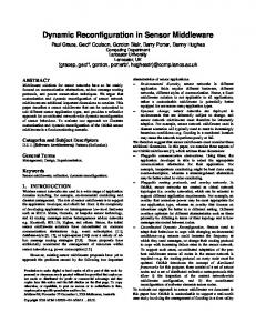
hereafter as segment (1) comprising the ball screw system, and an upper fixed-length part (designated Appl. Sci. 2016, 6, 80 3 of 19 hereafter as segment (2) consisting of the linear guide and connected rod. When the ball screws are driven by the motors, the connected rods move in a direction along the corresponding link axes such driven by the motors, the connected rods move in a direction along the corresponding link axes such that the positions and orientations of the platform type of end‐effector can vary according to a desired that the positions and orientations of the platform type of end-effector can vary according to a desired planning. Moreover, order to to optimally optimally adjust geometry for the task task planning. Moreover, inin order adjustthe thearchitecture architecture geometry for required the required performance, each universal joint Ai ,A i.e., the base point, can be displaced along the linear guideway of performance, each universal joint i , i.e., the base point, can be displaced along the linear guideway the base. In addition, the applied dynamic wrenchwrench force f force and wrench moment n are also introduced of the base. In addition, the applied dynamic f and wrench moment n are also to the center of mass of the moving platform for the maximum dynamic wrench capability analysis introduced to the center of mass of the moving platform for the maximum dynamic wrench capability of the reconfigurable parallel robot. Therefore, by displacing the base locations of each link along analysis of the reconfigurable parallel robot. Therefore, by displacing the base locations of each link along a linear guideway, the reconfigurable proposed reconfigurable parallel is capable of varying its to a linear guideway, the proposed parallel robot is robot capable of varying its geometry geometry to fulfill a specified task with the maximum dynamic wrench capability. fulfill a specified task with the maximum dynamic wrench capability.
Figure 1. Geometric structure of a reconfigurable motor-driven parallel robot. Figure 1. Geometric structure of a reconfigurable motor‐driven parallel robot.
In studying the optimal architecture of a reconfigurable parallel robot for maximum dynamic In studying the optimal architecture of a reconfigurable parallel robot for maximum dynamic wrench capability, an appropriate inverse dynamics form is required. In comparing with other wrench capability, an appropriate inverse dynamics form is required. In comparing with other formatting algorithms for the dynamic equations of parallel robots, several methods such as the formatting algorithms for the dynamic equations of parallel robots, several methods such as the Newton‐Euler formulation [12–14], virtual work principle [15,16], Kane’s method [17], kinematic Newton-Euler formulation [12–14], virtual work principle [15,16], Kane’s method [17], kinematic influence coefficient theory [18], screw theory [19], and the Lagrangian formulation in generalized influence coefficient theory [18], screw theoryand [19], and the Lagrangian formulation in generalized coordinates [20–22] are proposed to model simulate the dynamics of parallel manipulators. coordinates [20–22] are proposed to model and simulate the dynamics of parallel manipulators. However, these expressions are not structured enough, and are not appropriate for the dynamic wrench capability analysis. Therefore, following our previous development, the Boltzmann‐Hamel‐d’Alembert However, these expressions are not structured enough, and are not appropriate for the dynamic wrench formula will be used to develop the required dynamics. capability analysis. Therefore, following our previous development, the Boltzmann-Hamel-d’Alembert As shown in Figure 2, the associated frames are first assigned in developing the dynamics of the formula will be used to develop the required dynamics. parallel robot the dynamic wrench capability analysis. Here, an ininertial coordinate system of As shown in for Figure 2, the associated frames are first assigned developing the dynamics N‐frame, x N y N z N , is fixed to the base and a second coordinate system B‐frame, xb yb zb , is attached
the parallel robot for the dynamic wrench capability analysis. Here, an inertial coordinate system to the moving platform with its origin located at the platform’s center of mass, B, whose position N-frame, x N y N z N , is fixed to the base and a second coordinate system B-frame, xb yb zb , is attached vector with respect to the N‐frame is denoted as p. Moreover, two parallel local coordinate systems, to the moving platform with its origin located at the platform’s center of mass, B, whose position i.e., i1‐frame and i2‐frame with the corresponding origins Ai1 and Ai2, are attached to the segment 1 vector with respect to the N-frame is denoted as p. Moreover, two i1parallel local coordinate systems, and segment 2 of the link i, respectively, and the position vector of A with respect to the N‐frame is i.e., i1represented as a -frame and i2 -frame with the corresponding origins Ai1 and Ai2 , are attached to the segment 1 i. The position vector of the ball joint Bi with respect to the B‐frame is defined as b i, and segment 2 of the link i, respectively, and the position vector of A with respect to the N-frame and the length vector of link i from the universal joint Ai1 to the ball i1 joint Bi with respect to the is represented as ai . The position vector of the ball joint Bi with respect to the B-frame is defined as i1‐frame is expressed as li . Because the length vector of each link is an addition of the variable length bi , and the length vector of link i from the universal joint Ai1 to the ball joint Bi with respect to the i1 -frame is expressed as li . Because the length vector of each link is an addition of the variable length
Appl. Sci. 2016, 6, 80
4 of 19
Appl. Sci. 2016, 6, 80
4 of 18
vector l i 1 of the lower segment to the constant length vector li2 of the upper segment, the length vector of link i can be written as vector li1 of the lower segment to the constant length vector li2 of the upper segment, the length vector li li si li1 li 2 li1 +li2 si (1) of link i can be written as li “ li si “ li1 ` li2 “ pli1 ` li2 q si (1)
where s sis is an unit vector along the ith link axis and is expressed in the i 1‐frame; li, li1 and li2 are the i an where unit vector along the ith link axis and is expressed in the i1 -frame; li , li1 and li2 are the i respective length magnitudes of link i, as well as the lower segment and the upper segment of link i. respective length magnitudes of link i, as well as the lower segment and the upper segment of link i.
Figure 2. Coordinate systems of link and moving platform. Figure 2. Coordinate systems of link and moving platform.
Because in the parallel robot structure there exist multiple closed‐loop chain mechanisms, the Because in the parallel robot structure there exist multiple closed-loop chain mechanisms, the geometric constraint equation based on a vector loop relationship can be formulated as geometric constraint equation based on a vector loop relationship can be formulated as N
N
p NBBRb Rbi i“aaii ` Nii Rl p` Rlii
(2) (2)
NN In subscripts L PL tB, represents the with subscripts represents In Equation Equation (2), (2), the the rotation rotation matrix matrix L LRRwith { ipi B , i“( i1,..., 1, 6qu ..., 6)} transformation from a local L-frame to the inertial N-frame. The time derivative of this rotation matrix the transformation from a local L‐frame to the inertial N‐frame. The time derivative of this rotation can be expressed as . matrix can be expressed as N N r (3) L L R “ L Rω N N ” ıT L (3) LRfrom LRω r L is a skew symmetric matrix formed in which ω the angular velocity ωL “ ωx ωy ωz L T with respect to a local body-fixed L-frame, i.e., L is a skew symmetric matrix formed from the angular velocity ωL x y z in which ω » fi L 0 ´ωz ωy with respect to a local body‐fixed L‐frame, i.e., — ffi r L “ – ωz ω (4) 0 ´ωx fl ´ω 0 y ωx z 0 y L ω L z 0 x (4) Moreover, the angular velocity ωL canbe related to the time derivative of the Euler angles using x that0 L y CL such a corresponding velocity transformation matrix
Moreover, the angular velocity
ωLbe “related CL γ9 L to the time derivative of the Euler angles (5) ωL can
CL using Taking a derivative on the constraint Equation (2), and the fact that no spin is allowed about using a corresponding velocity transformation matrix such that its link axis due to the connection of each link to the base by an universal joint, i.e., (5) ωL CLγL ωiT si “ 0 (6)
Appl. Sci. 2016, 6, 80
5 of 18
Thus, the sliding velocity and the angular velocity of link i with respect to the i1 -frame can be obtained as .
.
´
N i Rsi
l i “ l i1 “ ωi “ .
¯T
´
.
p`
N i Rsi
¯T
N r B R ωB bi
(7)
¯ 1 N T ´. N r r B bi si i R p ` B R ω li
(8)
.
where l i “ l ι1 implies that the sliding velocity of each link is equivalent to the relative sliding velocity between the two segments of the link. Furthermore, the corresponding sliding acceleration and angular acceleration of link i can be obtained by differentiating the Equations (7) and (8) as ..
´ ¯ ´ .. T .. l i “ l i1 “ li ωiT ωi ` siT N R p` i .
ωi “
´ .. 1´ . ´2l i ωi ` rsi N R p` i li
N r r B R ωB ωB bi
N r r B R ωB ωB bi
`
`
¯ . N r B R ω B bi
¯¯ . N r B R ω B bi
(9) (10)
From Equations (7) and (8), the linear velocities of the links to the linear and angular velocities of the moving platform can be related by the following Jacobian matrix as . fi « . ff l1 — . ffi P — . ffi “ Jacob – . fl ωB . l6
»
where
pN Rs1 q — 1 . .. Jacob “ — –
T
pN 6 Rs6 q
T
»
pN 1 Rs1 q
T N rT B R b1
.. .
T N rT pN 6 Rs6 q B R b6
(11)
fi ffi ffi fl
(12)
In addition, each link is driven by a motor through a ball-screw transmission mechanism, so the effect of the ball-screw mechanisms on the dynamics is also included in accordance with .
.
l i “ pi αι {2π
(13) .
where the sliding velocity of the link i is related to the angular velocity αι of the corresponding motor by means of the pitch (i.e., the advanced distance per revolution) pi of the ith ball screw. Combining Equations (7) and (8), we can express, then expand these constraint equations in a velocity form as Jv “ J1 v1 ` J2 v22 “ 0 (14) ” ıT ” ı T . . .T where v “ “ is composed of the v1T v2T p ωBT l 11 . . . l 61 ω1T . . . ω6T corresponding velocities of the moving platform and the six links, and » — — — — J1 “ — — — –
1 N T rs1 R l1 1 .. .
Jacob T 1 p rs1 N RT q N Rr b1 1 B l1 .. .
1 N T rs6 R l6 6
1 rT p rs6 N RT q N B R b6 l6 6
J2 = ´I24ˆ 24 with Inˆn is a n ˆ n unit matrix.
fi ffi ffi ffi ffi ffi ffi ffi fl
(15)
Appl. Sci. 2016, 6, 80
6 of 18
From Equation (14), v2 can be parameterized by v1 as v2 “ J1 v1
(16)
and then by differentiating Equation (16), the parameterized acceleration is .
.
.
v2 “ J1 v1 ` J1 v1
(17)
On the basis of the developed structured Boltzmann-Hamel-d’Alembert formulism for a parallel mechanism [23–25], the dynamics of the PR can be given as « .
. pM1 v1 ` D1 v1 ` G1 q ` J1T pM2 v2
T ´1
` D2 v2 ` G2 q “ Jacob L
τ´
N Rf B
ff (18)
n
ıT ” . T in which v1 “ are the velocities of the moving platform, v2 “ P ωBT ” . ıT . are the sliding velocities and the angular velocities of the l 11 . . . l 61 ω1T . . . ω6T six links. Moreover, the matrices and vectors in Equation (18) are fully derived and explained in the Appendix. Also, it is noted that the applied dynamic wrench force f and wrench moment n are expressed in terms of the moving platform-fixed B-frame. Equation (18) can be further simplified using the kinematic relationships Equations (16) and (17) . to eliminate v2 and v2 so that the following equations of motion are yielded: .
Mp v1 ` Dp v1 ` Gp “ fp where Mp “
M1 ` J1T M2 J1 ,
Dp “
D1 ` JT1 D2 J1
(19) «
. ` J1T M2 J1 ,
Gp “
G1 `J1T G2 , fp
JacobT L´1 τ
N B Rf
ff
. n Because the expressions for the rotations of the moving platform are in terms of the quasi-velocities and the corresponding derivatives, a velocity transformation matrix relating quasi-velocities to the time derivative of angular orientation coordinates is required for further describing the orientations of the moving platform in space. The velocity transformation is defined as “
.
v1 “ C1 x
´
(20)
” . ıT . T .T in which x “ P , and γB , generally defined by a set of Euler angles, specifies the orientations γB of the moving platform. Also, the velocity transformation matrix C1 is defined as « C1 “
I3ˆ3 0
ff 0 CB
(21)
where CB is for the angular velocity transformation of the moving platform. Moreover, the applied wrenches can be expressed as «
f n
ff
« “
psα f qpcβ f q 0
psα f qpsβ f q 0
cα f 0
0 psαn qpcβ n q
0 psαn qpsβ n q
0 cαn
ffT «
fw nw
ff “ Tw Qw (22)
where fw and nw are the magnitudes of the dynamic wrench force and wrench moment; α and β are the angles of the applied wrenches with respect to the B-frame, and the subscripts f and n in Equation (22) respectively refer to the dynamic wrench force and wrench moment. For the problem of the dynamic wrench capability, we wish to find the allowable maximum dynamic wrench of the reconfigurable parallel robot along a specified trajectory without the violation
Appl. Sci. 2016, 6, 80
7 of 18
of constraints. Accordingly, the objective function is dynamic wrench capability that comprises the dynamic wrench force and wrench moment. Substituting Equation (20) together with its time derivative and Equation (22) into the equations of motion, Equation (19), gives rise to an inverse dynamics equation in true coordinates (p, γB ): «
« JacobT L´1
´
ff
NR B
0
0
I3ˆ3
ff «
ff τ Qw
Tw
..
.
“ Mp x ` Dp x ` Gp
(23)
.
where Mp “ Mp C1 , Dp “ Mp C1 ` Dp C1 , Gp “ Gp , or more compactly, Aeq ς “ beq ” in which ς “
τT
T Qw
ıT
(24)
include the input torques τ, and the dynamic wrench magnitudes
]T .
Qw = [fw nw It is seen that the proposed approach to the development of the governing dynamic model for the dynamic wrench capability analysis generates a structured linear parameter matrix-vector form with respect to the input torques and the magnitudes of the dynamic wrench force and wrench moment. 3. Reconfiguration for the Maximum Allowable DWC In the determination of the maximum allowable dynamic wrench capability while driving the adjustable parallel robot along a specified trajectory, the aim is to find the maximum possible magnitudes of the dynamic wrenches as well as the optimal link attachments of the parallel robot via a reconfiguration. In other words, the position vectors ai of the universal joints Ai1 for the link i are defined as the undetermined design variables. In general, the optimized geometry (i.e., the position vectors ai ) depends strongly upon the form of the cost function, the given trajectories, the applied wrench directions with respect to the moving platform and the associated constraints. Accordingly, an appropriate algorithm for optimizing the geometry considering the maximum allowable dynamic wrench capability is developed in this section. 3.1. Wrench Capability Formulation for a Predefined Trajectory To maximize the dynamic wrenches, a linear weighting combination of the dynamic wrench force and wrench moment is defined as the cost function ´ G“G
¯ a1 ,
...
, a6
“ λT ς “
” 01ˆ6
λf
λn
ıT ς
(25)
or equivalently to minimize the following fitness G “ ´G “ ´λT ς
(26)
in which the user-defined weighting coefficients λ f and λn are used to weight the relative importance of the considered applied dynamic wrench force and dynamic wrench moment. In order to ensure the practical feasibility of the adjustable parallel robot, the reconfiguration must take account of the physical constraints and design specifications imposed by the parallel robot structure as well as the actuator mechanism on the motion of the manipulator. Broadly speaking, the following inequalities are required to model these constraints: Each motor i has a designed maximum output torque value i τmax . Accordingly, the motor torque τ i is constrained as ˇ ˇ ˇ τi ˇ ˇ ˇ (27) ˇ i τ ˇ ď 1, for i “ 1, . . . , 6 max
In addition, due to the specified moving range of the base points Ai , the distance from the origin of the N-frame must be confined to
Appl. Sci. 2016, 6, 80
8 of 18
γimin ď |ai | ď γimax , for i “ 1, . . . , 6
(28)
In the current study, the aim of this optimization problem is to determine the optimal configuration along the given task trajectory considering the maximum allowable dynamic wrench capability. The allowable dynamic wrench capability is defined as the following: firstly, by discretizing the task trajectory under a presumed configuration ai , the dynamic wrench force f w and wrench moment nw at each spaced point are obtained by minimizing the fitness function given in Equation (26) subject to the equality constraint Equation (22) and the inequality constraints formulated in Equations (27) and (28). Then, the minimal dynamic wrench force and wrench moment are searched along the trajectory and then substituted into the Equation (25) so that the cost function value is defined as the allowable dynamic wrench capability for the task-dependent trajectory. Conventionally, a discretizing and searching method is applied to this constrained optimization problem by dividing each ai (i = 1, . . . , 6) into n discrete points between γimin ď |ai | ď γimax , and then for the specified trajectory, the corresponding allowable dynamic wrench capability for all the n6 configurations of the parallel robot can be determined by the constrained optimization method. Accordingly, the reconfiguration with the maximum allowable dynamic wrench capability can be made by comparing the n6 solutions. However, it is very time-consuming and arduous for a large n. Instead, a hierarchical optimization process is proposed in this paper. 3.2. Solution Procedure by a Hierarchical Optimization Process In order to determine the position vectors ai which maximize the allowable dynamic wrench capability of the associated motion, a hierarchical optimization process combining two optimization algorithms is proposed. As aforementioned, firstly for the initial presumed position vectors ai (i = 1, . . . , 6) of the base points and at each discretizing point of the designated trajectory, the fitness function, Equation (26), is minimized under the constraint equations. Thus, the generated optimization process can be realized as a typical linear programming such that the Simplex-type linear programming method can be directly applied to determine the maximal dynamic wrench capability at each discrete point of the given trajectory. Next, from the obtained values, the minimum dynamic wrench force and moment are chosen as the allowable wrenches, and then the allowable dynamic wrench capability for this task trajectory is evaluated by substituting the minimum dynamic wrenches into the cost function, Equation (25). Afterwards, the position vectors ai of the base points Ai are varied to maximize the allowable dynamic wrench capability. For this optimization process, a population-based optimization technique, differential evolution, is employed. The differential evolution method simulates a natural evolution with a stochastic direct search mechanism according to the distribution of solutions in the current population [26,27]. As the algorithm proceeds, all the chromosomes of the next generation are as good as or better than their counterparts in the current generation, and then the individual chromosomes gradually converge toward an optimal solution. Once the termination criteria have been attained (e.g., a specified number of iterations have been performed or the fitness error satisfies the minimum error requirement, for example), the algorithm terminates, and the current optimal chromosome is taken as the global optimal solution of the problem of interest. Due to a low computational complexity, differential evolution outperforms many other optimization methods in terms of convergence speed and robustness for some benchmark functions. Furthermore, differential evolution has very few control parameters to adjust and has therefore been applied to many diverse fields [28–30]. Based on the optimization procedures in the hierarchical optimization process, the differential evolution is a higher-level optimization solver for varying the position vectors of the base points, and the Simplex-type linear programming is designated as the lower-level optimization solver for the determination of the dynamic wrench capability. The procedures for the optimal geometry adjustment for a given trajectory can be described as follows:
Appl. Sci. 2016, 6, 80
9 of 18
The higher-level optimization process is randomly initialized with P parent individuals according to a uniform probability distribution in the D dimensional problem space. Each parent individual is a set of undetermined position vectors of the base points, namely ” ıT T , . . . , aT sT , p = 1, . . . , P, and refers to a candidate solution in ˆ p fi x p1 . . . xpD X “[ap,1 p,6 a D-dimensional space based on the differential evolution algorithm for the optimization problem. Also, these candidate solutions must respect the constraint Equation (28). p (2) In the lower-level optimization process, for each individual p = 1, . . . , P, compute and record f w,n p and nw,n , n “ 1, . . . , N, for N discrete equally spaced points of the given trajectory by solving the linear programming problem for the minimization of the fitness function, Equation (26) with the equality and inequality constraints Equations (24) and (27). (3) Find the minimum dynamic wrench force f p,w and wrench for the individual )p ! ) moment n p,w ! (1)
p
p
along the task trajectory by f p,w “ min f w,n , n “ 1, . . . , N and n p,w “ min nw,n , n “ 1, . . . , N . In the ith generation of the differential evolution solution procedure, the allowable dynamic wrench capability G p = λ f f p,w ` λn n p,w in Equation (25) is evaluated using the minimum dynamic wrench force, f p,w and dynamic wrench moment, n p,w of each individual from the step (3). (5) Generate mutant individuals by adding a randomly selected individual to the difference of two other randomly selected individuals in the parent population according to the following equation:
(4)
ˆ r1 piq ` f m rX ˆ r2 piq ´ X ˆ r3 piqs Zˆ p pi ` 1q “ X
(29)
where p = 1,2, . . . , P is the individual’s index of population; i is the generation; Zˆ p piq “ rz p1 piq, z p2 piq, . . . , z pD piqsT represents the pth mutant vector via the mutation operation; r1, r2 and r3 are mutually different indices and also different from the running index, p, randomly selected with uniform distribution from the set {1, 2, . . . , p ´ 1, p + 1, . . . , P}; and fm > 0 is a mutation factor usually taken from the range [0.1, 1], and used to control the amplification of the difference between two parent individuals so as to avoid search stagnation. (6) For the components of each mutant vector, an index Rand(p)P{1, 2, . . . , D} is randomly chosen using uniform distribution, and the crossover is employed to create a trial vector ˆ p pi ` 1q “ ru p1 pi ` 1q, u p2 pi ` 1q, . . . , u pD pi ` 1qsT by recombining parent and mutant vectors as U the followings: # u p,j pi ` 1q “
z p,j pi ` 1q, prandpjq ď CRq pj “ Randppqq if or x p,j piq, prandpjq ą CRq pj ‰ Randppqq
(30)
where j = 1,2, . . . , D is the component index in D-dimensional individual, and rand(j) is the jth evaluation of a uniform random number generation with [0, 1], and CR is a crossover or recombination rate in the range [0, 1]. (7) Repeat the steps (2)–(4) to calculate the allowable dynamic wrench capability in G using the trial ˆ p pi ` 1q, p = 1, . . . , P, and then the cost function value of each trial vector U ˆ p pi ` 1q is vectors U ˆ p piq. This selection procedure is to decide if the compared with that of its parent target vector X ˆ p pi ` 1q becomes a member of the population of the next generation. Thus, trial vector U # ˆ p pi ` 1q “ X
ˆ p pi ` 1q, U ˆ p piq, X
if otherwise
ˆ p pi ` 1qq ą GpX ˆ p piqq GpU
(31)
ˆ p piq In this case, if the allowable dynamic wrench capability in G of the target parent vector X is larger than that of the trial vector, the target is allowed to advance to the next generation. Otherwise, the trial vector replaces the target vector to become a better offspring in the next generation.
Appl. Sci. 2016, 6, 80
(8)
10 of 18
Repeat the steps beginning from step (2) until it has reached a stopping criterion in accordance with the user-defined conditions, usually a maximum generation number is set for the stop ˆ best is the best individual vector for the optimal configuration with the best criterion. Thus, X objective function value in this population.
4. Examples In this section, the optimal locations of the base points for the reconfigurable parallel robot considering the maximum allowable dynamic wrench capability will be determined through numerical simulations. This section commences with the assumptions made in building the parallel robot system and in modeling its kinedynamic response, and then the simulation results are presented when specifying different types of adjustments on the base point locations for a prescribed task trajectory. 4.1. Kinematic Parameters and Differential Evolution Variables The system parameters used for the simulation are given as the following, (1)
Platform points in the B-frame: ” B2j´1 “ r B cospp2j ´ 1qπ{3 ´ π{18
sinpp2j ´ 1qπ{3 ´ π{18q 0
” B2j “ r B
cospp2j ´ 1qπ{3q sinpp2j ´ 1qπ{3
0
ıT
ıT
,
, j “ 1, . . . , 3
with the radius of the moving platform r B = 0.3 m. (2) Base points in the N-frame: ” ıT A2j´1 “ r A2j´1 cosp2pj ´ 1qπ{3q sinp2pj ´ 1qπ{3 0 , ” A2j “ r A j
cosp2pj ´ 1qπ{3 ` π{18q sinp2pj ´ 1qπ{3 ` π{18
0
ıT
, j “ 1, . . . , 3.
in which r Ai , i “ 1, . . . , 6 is the distance of the ith base point from the origin of the inertial N-frame. Inasmuch as the disposed base locations may not exceed the specified ranges, the distance of the ith base point can be assigned as r Ai “ p1 ´ ηi qr B ` ηi r Amax , 0 ď ηi ď 1
(32)
where r Amax is the maximum allowable distance of the base points, and ηi (i = 1, . . . , 6) are the proportional coefficients such that the positions of each base point will be confined between r B and r Amax = 1.5 m. As a result, the optimal geometry for the reconfigurable parallel robot with the maximum dynamic wrench capability is equivalent to finding the proportional coefficients. Furthermore, all the links are considered to be identical and to have a lower segment of mass mi1 = 2 kg as well as an upper segment of mass mi2 = 1 kg. The lower segment of each link incorporates a ball-screw system with a pitch pi of 5 mm/rev. The unit vector si expressed in the i1 -frame is given by si =r 1
T
0 s . The gravity centers of the two segments of each link are respectively
0 T
T
di1 “ r 0.5 0 0 s m and di2 “ r 0.5 0 0 s m. The constant length of the upper segment 2 is li2 = 1.0 m. The moments of inertia of these two segments of each link about their respective gravity centers in the local frame are C Ii1 “ diag[0.001, 1, 1] kg¨ m2 , C Ii2 “ diag[0.0001, 0.4, 0.4] kg¨ m2 . The moments of inertia of the segments 1 and 2 of each link about the respective joint points Ai1 and Ai2 in rT d rij , j = 1, 2. The the local frame can be calculated using the parallel axes theorem as Iij “C I ` mij d ij
T
m/s2 .
ij
vector of gravity is g “ r 0 0 ´9.81 s The trajectory of the center of mass B of the moving platform is given as p = [0.25sinp0.4π tq 0.3cosp0.4πtq 1.2 ` 0.1sinp0.8πtq]T and γB “[0.2sinp0.2πtq 0.3cosp0.4πtq 0.25sinp0.1πtq]T , and the applied directions of the dynamic wrench force and wrench moment are individually specified as
Appl. Sci. 2016, 6, 80
11 of 18
(α f , β f ) = (π/6, π/3), and (αn , βn ) = (π/3, π/6) with respect to the B-frame. Moreover, it is assumed that this trajectory satisfies the kinematic constraints of the parallel robot systems, i.e., the link lengths, velocities ” ı and accelerations. In addition, the maximum motor torques are specified as |τ1 |
...
|τ6 |
ď [3.5 4 2.5 2.5 3 3.5] Nm.
The rotation matrix N L R with subscripts L P tB, ipi “ 1, ..., 6qu is defined as »
cψcθ — N R “ – sψcθ L ´sθ
fi ´sψcφ ` cψsθsφ sψsφ ` cψsθcφ ffi cψcφ ` sψsθsφ ´cψsφ ` sψsθcφ fl cθsφ cθcφ
(33) L
where c p¨ q is a shorthand notation for cos p¨ q and s p¨ q for sin p¨ q. The Euler angles vector ” ıT γ“ ψ θ ϕ is used to specify the orientation, which means that the inertial frame is rotated about the Z axis with ψ first, resulting in the primed frame; then about the y1 axis with θ, resulting in the double primed frame; and finally about the x2 axis with φ, resulting in the local frame. Moreover, the corresponding velocity transformation matrix » ´sθ — CL “ – cθsφ cθcφ
0 cφ ´sφ
fi 1 ffi 0 fl 0
(34) L
4.2. Results and Discussion Appl. Sci. 2016, 6, 80
12 of 19
In solving the maximum dynamic wrench capability problem of the reconfigurable parallel In solving the maximum dynamic wrench capability problem of the reconfigurable parallel robot, the positive weighting numbers in Equations (25) and (26) are specified as [λ f λn ] = [1.0 2.0] robot, the positive weighting numbers in Equations (25) and (26) are specified as [λ f λn] = [1.0 2.0] considering the desired relative magnitudes of the dynamic wrench force and wrench moment for considering the desired relative magnitudes of the dynamic wrench force and wrench moment for this given trajectory. Then, an initial determination of the maximum DWC was carried out in which this given trajectory. Then, an initial determination of the maximum DWC was carried out in which the proportional coefficients for the base point locations were set to be ηi η= 0.1, (i = 1, …, 6), or the i = 0.1, (i = 1, . . . , 6), or the the proportional coefficients for the base point locations were set to be corresponding distances of the base points are r Ai =r 0.42 m. The trajectory is discretized into 51 points corresponding distances of the base points are Ai = 0.42 m. The trajectory is discretized into 51 with the time step ∆t = 0.1 s. The maximum dynamic wrench capability at each point is calculated points with the time step Δt = 0.1 s. The maximum dynamic wrench capability at each point is by the Simplex-type linear programming method, and hence the dynamic wrench force and wrench calculated by the Simplex‐type linear programming method, and hence the dynamic wrench force momentand wrench moment at each point of the prescribed trajectory is shown in Figure 3. It is shown that at each point of the prescribed trajectory is shown in Figure 3. It is shown that the minimum dynamic wrench force is 189.6962 N at time t = 2.3 s and the minimum dynamic wrench moment the minimum dynamic wrench force is 189.6962 N at time t = 2.3 s and the minimum dynamic wrench moment is 38.3488 Nm at time t = 5.0 s. Thus, the allowable dynamic wrench capability is 266.3938 is 38.3488 Nm at time t = 5.0 s. Thus, the allowable dynamic wrench capability is 266.3938 for the for the specified initial base points. specified initial base points.
FigureFigure 3. Variations of dynamic wrenches at each point of prescribed trajectory. 3. Variations of dynamic wrenches at each point of prescribed trajectory. As in the aforementioned, the proposed hierarchical optimization approach combining the differential evolution and the Simplex‐type linear programming is used to perform a series of simulations in which the optimal base point locations for an improvement of the allowable dynamic wrench capability are obtained. Furthermore, the performance of a differential evolution algorithm for the formulated maximum dynamic wrench capability problem usually depends on three variables: the population size P, the mutation factor fm, and the recombination rate CR. Thus, in
Appl. Sci. 2016, 6, 80
12 of 18
As in the aforementioned, the proposed hierarchical optimization approach combining the differential evolution and the Simplex-type linear programming is used to perform a series of simulations in which the optimal base point locations for an improvement of the allowable dynamic wrench capability are obtained. Furthermore, the performance of a differential evolution algorithm for the formulated maximum dynamic wrench capability problem usually depends on three variables: the population size P, the mutation factor fm , and the recombination rate CR. Thus, in accordance with the results of a few trial and error simulations, in which P = 25, fm = 0.5 and CR = 0.8 are specified here for a trade-off consideration. In the example, the base points are displaced equidistantly such that only one proportional coefficient η is determined for the maximum allowable dynamic wrench capability. Figure 4 shows that the proposed hierarchical optimization algorithm for the maximum allowable dynamic wrench capability leads to a high convergence rate. The obtained convergent proportional coefficients in Figure 5 are ηi = 0.3684, (i = 1, . . . , 6), or the corresponding distances of the base points are r Ai = 0.7421 m. The corresponding allowable maximum dynamic wrench capability, the dynamic wrench force and wrench moment are 408.4895, 224.8770 N and 91.8063 Nm, respectively. It is found that the allowable dynamic wrench capability has been improved. Figure 6 presents the variations of the dynamic wrenches along the prescribed trajectory for this configuration. The minimum dynamic Appl. Sci. 2016, 6, 80 13 of 19 wrench force/moment are still at time t = 2.3 s and at time t = 5.0 s, respectively. Appl. Sci. 2016, 6, 80
13 of 19
Figure 4. Allowable dynamic wrench capability versus iteration number for base point locations being Figure 4. Allowable dynamic wrench capability versus iteration number for base point locations being Figure 4. Allowable dynamic wrench capability versus iteration number for base point locations being displaced equidistantly. displaced equidistantly. displaced equidistantly.
Figure 5. Base point position versus iteration number for base point locations being displaced equidistantly. Figure 5. Base point position versus iteration number for base point locations being displaced equidistantly. Figure 5. Base point position versus iteration number for base point locations being displaced equidistantly.
Appl. Sci. 2016, 6, 80
13 of 18
Figure 5. Base point position versus iteration number for base point locations being displaced equidistantly.
η
Figure 6. Variations of dynamic wrenches along prescribed trajectory for η = 0.3684. Figure 6. Variations of dynamic wrenches along prescribed trajectory for i i = 0.3684.
Moreover, Table 1 lists the convergence analyses for different population size P = 15, 25, 35. Moreover, Table 1 lists the convergence analyses for different population size P = 15, 25, 35. As As shown, the population size P = 35 goes through fewer iterations to reach the specified convergence shown, the population size P = 35 goes through fewer iterations to reach the specified convergence Appl. Sci. 2016, 6, 80 14 of 19 criteria of of thethe wider and more coverage of the search space; however, thehowever, computation criteria because because wider and random more random coverage of the search space; the time increases with an increase in the required function evaluation. Therefore, the population size computation time increases with an increase in the required function evaluation. Therefore, the P = 25population size P = 25 is adopted for the differential evolution algorithm. Finally, the base points of is adopted for the differential evolution algorithm. Finally, the base points of the parallel robot are relocated individually to further improveto the maximum allowable dynamic wrench capability the parallel robot are relocated individually further improve the maximum allowable dynamic usingwrench capability using the proposed hierarchical optimization. Figures 7 and 8 respectively present the proposed hierarchical optimization. Figures 7 and 8 respectively present the convergence process the maximum dynamic wrenchdynamic capability andcapability the six base point the for convergence process allowable for the maximum allowable wrench and the six positions. base The obtained proportional coefficients are [η1 ,. . .,η6 ] = [0.2038, 1.0000, 0.0000, 1.0000, 0.4576, 1.0000], point positions. The obtained proportional coefficients are [ η1 , , η6 ] = [0.2038, 1.0000, 0.0000, and the corresponding maximum fitness value = 583.9285, the dynamic wrench force is 514.9908 N 1.0000, 0.4576, 1.0000], and the corresponding maximum fitness value = 583.9285, the dynamic and the dynamic wrench moment is 34.4688 Nm. Also, the corresponding dynamic wrenches along wrench force is 514.9908 N and the dynamic wrench moment is 34.4688 Nm. Also, the corresponding the prescribed trajectory are shown in Figure 9. It can be found that the improved allowable dynamic dynamic wrenches along the prescribed trajectory are shown in Figure 9. It can be found that the wrench capability stems dynamic mainly from thecapability increase of the mainly minimum dynamic wrench force. improved allowable wrench stems from the increase of the minimum dynamic wrench force. Table 1. Convergence analyses for different particle numbers. Table 1. Convergence analyses for different particle numbers.
Population Size P Population Size P No. of Iteration No. of Iteration Computation Time (s) Computation Time (s) Fitness Value Fitness Value
15 15 40 40 1.315 ˆ10102 2 1.315 221.5172 221.5172
25 25 40 40 2 3.286 3.286ˆ 10 2 408.4895 408.4895
35 35 2525 3 4.391 ˆ10 4.391 103 408.4831 408.4831
Figure 7. Maximum allowable dynamic wrench wrench capability number for base point point Figure 7. Maximum allowable dynamic capabilityversus versusiteration iteration number for base locations being displaced individually. locations being displaced individually.
Figure 7. Maximum allowable dynamic wrench capability versus iteration number for base point 14 of 18 locations being displaced individually.
Appl. Sci. 2016, 6, 80
Figure 8. Base point positions versus iteration number for base point locations being Figure 8. Base point positions versus iteration number for base point locations being displaced individually. Appl. Sci. 2016, 6, 80 15 of 19 displaced individually.
η
η
Figure 9. Variations of dynamic wrenches along prescribed trajectory for [η1 ,. . .,η6 ] = [0.2038, 1.0000, Figure 9. Variations of dynamic wrenches along prescribed trajectory for [ 1 , , 6 ] = [0.2038, 0.0000, 1.0000, 0.4576, 1.0000]. 1.0000, 0.0000, 1.0000, 0.4576, 1.0000].
Table 2 gives the comparisons for the initial base point locations, the equidistant displaced base Table 2 gives the comparisons for the initial base point locations, the equidistant displaced base point locations and the respectively displaced base point locations. It is seen that the base locations point locations and the respectively displaced base point locations. It is seen that the base locations have a critical effect on the allowable dynamic wrench capability of the reconfigurable parallel robot. have a critical effect on the allowable dynamic wrench capability of the reconfigurable parallel robot. Especially, in this case study, the allowable dynamic wrench capability for the optimal configuration Especially, in this case study, the allowable dynamic wrench capability for the optimal configuration with the respectively displaced base point locations can be increased 119.2%, better than that with the with the respectively displaced base point locations can be increased 119.2%, better than that with equidistantly displaced base locations which increases by 53.34% in the allowable dynamic wrench the equidistantly displaced base locations which increases by 53.34% in the allowable dynamic capability. Moreover, if we look into the torques for these three configurations as shown in Figure 10, wrench capability. Moreover, if we look into the torques for these three configurations as shown in some actuators saturate in order to maximize the dynamic wrench capability. Especially, at time t = 2.3 s, Figure 10, some actuators saturate in order to maximize the dynamic wrench capability. Especially, it can be seen that the dominant actuator 3 can exert larger torque through the optimal reconfiguration at time t = 2.3 s, it can be seen that the dominant actuator 3 can exert larger torque through the optimal so that the minimal dynamic wrench force improves more. Finally, the numerical efficiency comparison reconfiguration so that the minimal dynamic wrench force improves more. Finally, the numerical is shown in Table 3. It is seen that a large amount of time is taken for computation for the conventional efficiency comparison is shown in Table 3. It is seen that a large amount of time is taken for discretizing and searching method as compared to the proposed hierarchical optimization algorithm. computation for the conventional discretizing and searching method as compared to the proposed hierarchical optimization algorithm. Table 2. Results for three different types of base locations.
Results
[ η1 , , η6 ]
Allowable DWC
[fw, nw]
Initial base point locations
[0.1, …, 0.1]
266.394
[189.696, 38.349]
Appl. Sci. 2016, 6, 80
15 of 18
Table 2. Results for three different types of base locations. Results
[η1 , . . . , η6 ]
Allowable DWC
[fw , nw ]
Initial base point locations
[0.1, . . . , 0.1]
266.394
[189.696, 38.349]
Equidistant displaced base point locations
[0.3684, . . . , 0.3684]
408.490
[224.877, 91.806]
Respectively displaced base point locations
[0.2038, 1.0, 0.0, 1.0, 0.4576, 1.0]
583.929
[514.991, 34.469]
Appl. Sci. 2016, 6, 80
16 of 19
(a)
(b)
(c) Figure 10. 10. Torques Torques with with the the maximum maximum dynamic dynamic wrench wrench capability capability for Figure for (a) (a) initial; initial; (b) (b) equidistantly equidistantly displaced; (c) individual displaced base point locations. displaced; (c) individual displaced base point locations.
5. Conclusions This study proposes a reconfigurable Stewart‐based parallel robot and a scheme for the optimal reconfiguration according to the maximum allowable dynamic wrench capability instead of a trial‐and‐error selection. In the proposed approach, the closed‐form inverse dynamics equation, which is linear with respect to the required dynamic wrenches and input torques, is first developed
Appl. Sci. 2016, 6, 80
16 of 18
Table 3. Numerical efficiency analysis for different methods. Algorithm
Discretizing & Searching
Hierarchical Optimization
Number
n = 25
p = 25
Computation time (s) Fitness value
6.272 ˆ 104
8.125 ˆ 102 583.929
571.8061
5. Conclusions This study proposes a reconfigurable Stewart-based parallel robot and a scheme for the optimal reconfiguration according to the maximum allowable dynamic wrench capability instead of a trial-and-error selection. In the proposed approach, the closed-form inverse dynamics equation, which is linear with respect to the required dynamic wrenches and input torques, is first developed via a structured Boltzmann-Hamel-d’Alembert formula. Then, a hierarchical optimization process, combining the differential evolution algorithm for the higher-level optimization and the Simplex-type linear programming scheme for the lower-level optimization, is presented to search for the optimal base point locations for the maximal allowable dynamic wrench capability. It is clear that optimally varying the base point locations leads to a very pronounced increase in the maximum allowable dynamic wrench capability. Finally, the presented generic analysis technique in this study can easily be generalized to the maximum dynamic wrench capability analyses of any other reconfigurable parallel robot domain, and suggests a practically useful way to promptly vary the parallel robot’s geometry. The reconfigurable parallel robots offer considerably larger potential in optimizing velocities, force capabilities that in general may be presented by manipulability and force ellipsoids, energy-consumption, reduced machining time etc. These topics will be pursued as future works. Moreover, the presented analyses in this paper can be extended to dodecapod-parallel robots with on-line adaptable basis joint positions. Author Contributions: Chun-Ta Chen conceived the topic and developed the equations; Chih-Jer Lin and Chun-Ta Chen analyzed the results and wrote the paper. Conflicts of Interest: The authors declare no conflict of interest.
Appendix Inertia matrix: « m B I3ˆ3 M1 “ 03ˆ3 » M2 “ –
ff 03ˆ3 IB
, ”
diag rm12 , . . . , m62 s
diag
”
T
r m12 s1T d ” 12 diag I1
ı r62 s6 m62 d ´ ¯ 2r ri2 ` d rT rsi , i “ 1, . . . , 6 and Ii “ Ii1 ` Ii2 ´ mi2 li1 s2i ` mi2 li1 rsiT d i2 diag
r12 s1 m12 d
,...,
T
r m62 s6T d ı 62 , . . . , I6 ,...,
ı fi fl,
Coriolis and centrifugal terms: « ff 03ˆ3 03ˆ3 D1 “ , 03ˆ3 pIB b ωB qT » D2 “ –
” 06ˆ ” diag
T
r qrs1 ω1 m12 pl11rs1T ` d 12
.
,...,
T
diag T
r qrs6 ω6 m62 pl61rs6T ` d 62
ı
r q , . . . , m62 ω Trs6 pl61rs6 ` d r62 q m12 ω1Trs1 pl11rs1 ` d ” 12 ı 6 diag h1 , . . . , h6
r qrsi ` ppIi1 ` Ii2 q b ωi qT ` mi2 li1 pω T di2 qrsT , i “ 1, . . . , 6 where hi “ mi2 l i1 pli1rsiT ` d i2 i i
ı fi fl ,
Appl. Sci. 2016, 6, 80
17 of 18
gravity vector: « ff ´m B g G1 “ , 03ˆ1 » G2 “ – ”
”
r ´gT N 1 Rpm11 d11
´m12 gT N 1 Rs1
r12 qT ` m12 l11rsi ` m12 d ıT
” The actuating torques: τ “ » — — — — J1 “ — — — –
1 N T rs1 R l1 1 .. .
τ1
...
τ6
Jacob
fi
T 1 p rs1 N RT q N Rr b1 1 B l1 .. .
ffi ffi ffi ffi ffi, ffi ffi fl
1 N T 1 N T N rT rs6 R p r s 6 R q B R b6 l6 6 l6 6 ” ı L “ diag p1 {2π . . . p6 {2π .
ı
...
´m62 gT N 6 Rs6
...
r ´gT N 6 Rpm61 d61
T ` m62 l61r si ` m62 dr62 q
fi ıT fl
.
It is noted that the symbol “b” in D1 and hi denotes a skew-symmetric matrix formed from the matrix-vector product. The skew-symmetric matrix is like the form in Equation (5). References 1. 2. 3. 4. 5.
6. 7. 8. 9. 10. 11. 12. 13. 14.
Plessis, L.J.; Snyman, J. An optimally re-configurable planar Gough-Stewart machining platform. Mech. Mach. Theory 2006, 41, 334–357. [CrossRef] Bi, Z.M.; Wang, L.H. Optimal design of reconfigurable parallel machining systems. Robot. Comput. Integr. Manuf. 2009, 25, 951–961. [CrossRef] Xi, F.; Xu, Y.; Xiong, G. Design and analysis of a re-configurable parallel robot. Mech. Mach. Theory 2006, 41, 191–211. [CrossRef] Ji, Z.; Song, P. Design of a reconfigurable platform manipulator. J. Rob. Syst. 1998, 15, 341–346. [CrossRef] Borras, J.; Thomas, F.; Ottaviano, E.; Ceccarelli, M. A reconfigurable 5-DoF 5-SPU parallel platform. In Proceedings of the ASME/IFToMM International Conference Reconfigurable Mechanisms Robots, London, UK, 22–24 June 2009; pp. 617–620. Kumar, S.G.; Nagarajan, T.; Srinivasa, Y.G. Characterization of reconfigurable Stewart platform for contour generation. Robot. Comput. Integr. Manuf. 2009, 25, 721–731. [CrossRef] Ji, Z. Analysis of design parameters in platform manipulators. ASME J. Mech. Des. 1996, 118, 526–531. [CrossRef] Vaida, C.; Plitea, N.; Lese, D.; Pisla, D. A parallel reconfigurable robot with six degrees of freedom. Appl. Mech. Mater. 2012, 162, 204–213. [CrossRef] Yeung, B.; Mills, J. Design of a six DOF reconfigurable gripper for flexible fixtureless assembly. IEEE Trans. Syst. Man Cybern. Part C 2004, 34, 226–235. [CrossRef] Coppola, G.; Zhang, D.; Liu, K. A 6-DOF reconfigurable hybrid parallel manipulator. Robot. Comput. Integr. Manuf. 2014, 30, 99–106. [CrossRef] Finistauri, A.D.; Xi, F. Reconfiguration analysis of a fully reconfigurable parallel robot. ASME J. Mech. Robot. 2013, 5, 17–34. [CrossRef] Do, W.; Yang, D. Inverse dynamic analysis and simulation of a platform type of robot. J. Robot. Syst. 1998, 5, 209–227. [CrossRef] Dasgupta, B.; Mruthyunjaya, T.S. A Newton-Euler formulation for the inverse dynamics of the Stewart platform manipulator. Mech. Mach. Theory 1998, 33, 1135–1152. [CrossRef] Dasgupta, B.; Mruthyunjaya, T.S. Closed-form dynamic equations of the general Stewart platform through the Newton-Euler approach. Mech. Mach. Theory 1998, 33, 993–1012. [CrossRef]
Appl. Sci. 2016, 6, 80
15. 16. 17. 18.
19. 20. 21. 22. 23. 24. 25. 26. 27. 28. 29. 30.
18 of 18
Wang, J.; Gosselin, C.M. A new approach for the dynamic analysis of parallel manipulators. Multibody Syst. Dyn. 1998, 2, 317–334. [CrossRef] Tsai, L.W. Solving the inverse dynamics of a Stewart-Gough manipulator by the principle of virtual work. Trans. ASME J. Mech. Des. 2000, 122, 3–9. [CrossRef] Liu, M.J.; Li, C.X.; Li, C.N. Dynamics analysis of the Gough-Stewart platform manipulator. IEEE Trans. Robot. Autom. 2000, 16, 94–98. Wang, S.C.; Hikita, H.; Kubo, H.Y.; Zhao, S.; Huang, Z.; Ifukube, T. Kinematics and dynamics of a 6 degree-of-freedom fully parallel manipulator with elastic joints. Mech. Mach. Theory 2003, 38, 439–461. [CrossRef] Carbonari, L.; Battistelli, M.; Callegari, M.; Palpacelli, M.C. Dynamic modelling of a 3-CPU parallel robot via screw theory. Mech. Sci. 2013, 4, 185–197. [CrossRef] Gregorio, R.D.; Parenti-Castelli, V. Dynamics of a class of parallel wrists. Trans. ASME J. Mech. Des. 2004, 126, 436–441. [CrossRef] Lebret, G.; Liu, K.; Lewis, F.L. Dynamic analysis and control of a Stewart platform manipulator. J. Robot. Syst. 1993, 10, 629–655. [CrossRef] Pang, H.; Shahinpoor, M. Inverse dynamics of a parallel manipulator. J. Robot. Syst. 1994, 11, 693–702. [CrossRef] Chen, C.T.; Liao, T.T. Optimal path programming of the SPM using the Boltzmann-Hamel-d’Alembert dynamics formulation model. Adv. Robot. 2008, 22, 705–730. [CrossRef] Chen, C.T. Hybrid approach for dynamic model identification of an electro-hydraulic parallel platform. Nonlinear Dyn. 2012, 67, 695–711. [CrossRef] Chen, C.T.; Pham, H.V. Trajectory planning in parallel kinematic manipulators using a constrained multi-objective evolutionary algorithm. Nonlinear Dyn. 2012, 67, 1669–1681. [CrossRef] Storn, R.; Price, K. Differential evolution? A simple and efficient heuristic for global optimization over continuous spaces. J. Glob. Optim. 1997, 11, 341–359. [CrossRef] Storn, R. System design by constraint adaptation and differential evolution. IEEE Trans. Evol. Comput. 1999, 3, 22–34. [CrossRef] Hrstka, O.; Kucerova, A. Improvement of real coded genetic algorithm based on differential operators preventing premature convergence. Adv. Eng. Softw. 2004, 35, 237–246. [CrossRef] Price, K.V.; Storn, R.M.; Lampinen, J.A. Differential Evolution: A Practical Approach to Global Optimization; Springer: Heidelberg, Germany, 2005. Coelho, L.S.; Mariani, V.C. Combining of chaotic differential evolution and quadratic programming for economic dispatch optimization with valve-point effect. IEEE Trans. Power Syst. 2006, 21, 989–996. © 2016 by the authors; licensee MDPI, Basel, Switzerland. This article is an open access article distributed under the terms and conditions of the Creative Commons by Attribution (CC-BY) license (http://creativecommons.org/licenses/by/4.0/).