RECONNECT: A flexible Router Architecture for Network-on-Chips

RECONNECT: A flexible Router Architecture for Network-on-Chips A Thesis Submitted for the Degree of

Doctor of Philosophy in the Faculty of Engineering

by

Alexander Fell

Supercomputer Education and Research Centre INDIAN INSTITUTE OF SCIENCE BANGALORE – 560 012, INDIA NOVEMBER 2012

ii

Acknowledgements I would like to take the opportunity and thank my advisor, Prof. S.K. Nandy, whose insights, encouragement and suggestions helped tremendously to finish this work successfully. Further I am grateful for his patience and support he showed towards me during my administrative and legal obligations such as visa applications and extensions. Secondly I express my gratitude towards Dr. Ranjani Narayan, CTO of Morphing Machines, for her moral and technical support during my stay in India. I am sure this work would have not been possible without her help. Besides I would like to thank my lab mates, especially Mythri Alle, Keshavan Varadarajan, Ganesha K. Garga, S. Balakrishnan and many more for testing my implementations and reporting bugs. They always had time to listen to problems that occurred. Their (sometimes unconventional) suggestions from a different point of view helped solving problems on many occasions. This thesis would not have been possible without the help of Niraj Sharma of Bluespec, Inc. During the realization of RECONNECT he always patiently listened to big and small implementation problems alike. Some of his suggestions for workarounds can still be found in the code and the forwarding the bugs reported to him, improved the Bluespec System Verilog (BSV) compiler. This acknowledgement would not be complete without the mentioning of the International Relation Cell (IRC) of IISc whose guidance and experience in visa related issues and organizational skills made my stay a very pleasant one. I was able to learn many interesting qualities about the Indian culture and I am sure that this exposure effectively changed my perception of life. Lastly I would like to thank all my friends from within and outside the institute for welcoming me into their families to give me an insight view into their lives. Further they were always present for an exhausting game of basketball to release excessive energy.

iv

Abstract In this thesis a Network on Chip (NoC) router implementation called RECONNECT realized in BSV, is presented. It is highly configurable in terms of flit size, the number of provided Input Port (IP)/Output Port (OP) pairs and support for configurations during runtime, to name a few. Depending on the amount of available IP/OP pairs, the router can be integrated into different topologies. Due to the ability to be configured during runtime, the router can even support multiple topologies. A developer is then able to choose among the available topologies the one that promises the highest performance for an application. However this work only concentrates on tessellations like toroidal mesh, honeycomb and hexagonal. Routing algorithms that were needed to be developed or adapted, are presented. In addition a step-by-step example of the routing algorithm development for the honeycomb topology is included in this thesis. This enables a system designer who wishes to use RECONNECT for any other topology that is not discussed such as a hypercube or a ring, to develop the required routing algorithm easily and fast. The impact of the chosen topology on the execution time of several real life algorithms has been analyzed by executing these algorithms on a target architecture called REDEFINE, a dataflow multi-processor consisting of Compute Elements (CEs) and Support Logic (SL). For this purpose an NoC comprising of RECONNECT routers establishing communication links among the CEs, has been integrated into REDEFINE. It has been found out that for very small algorithms, the execution time does not depend on the choice of topology, whereas for larger applications such as Advanced Encryption Standard (AES) encryption and decryption, it becomes evident that the honeycomb topology performs worst and the hexagonal one best. However it is observed that in many cases the additional links that are provided by the hexagonal topology, when compared with the mesh, are not utilized due to the topology unawareness of the REDEFINE SL. Hence the algorithm execution time for mesh topology is often on par with hexagonal ones. In addition to the chosen topology it is investigated, how the size of the flit affects these algorithms. As expected the performance of the NoC decreases, if the flit size is reduced so that the packets have to be segmented into more flits. Further it is analyzed, if the NoC performance is sufficient

vi to support high level algorithms such as e.g. the H.264 decoder through which data is streamed. These algorithms require to perform the necessary computations not only within a time constraint, but also the data needs to be fed to the Processing Elements (PEs) fast enough. In H.264 the time constraint is the frame rate meaning that each frame need to be processed in a specified fraction of a second. The current RECONNECT implementation does not qualify to deliver the data within this requirement. As a result, the necessity for a pipelined router version is presented. To allow a fair comparison of network performance with implementations found in current literature and to validate this approach, the NoC has been put under stress by artificial traffic generators which could be configured to generate uniform and self-similar traffic patterns. Further different destination addresses generation algorithms such as normal (randomly selecting a destination located anywhere in the network), close neighbor communication, bit complement and tornado, for each of these traffic patterns have been developed. It could be observed that in general the honeycomb topology performs worst, followed by the mesh and topped by the hexagonal topology. From the artificial traffic generators it can be concluded that the richer the topology, the higher the throughput. The different router designs have been synthesized to gain approximate area and power consumption details. Depending on the flit size the single cycle router which is able to forward an incoming flit in the next clock cycle, if no congestion occurs, dissipates between 13 and 35mW for honeycomb topology operating at a frequency of 450MHz. The power increases by approximately 25% for each IP/OP pair that is added to the router integrated in a honeycomb topology. The area that is required for a router in a honeycomb network, has been found out to be between 96167 and 301339 cells depending on the flit size. A router supporting a mesh or a hexagonal topology needs respectively 50% or 91% more area than the honeycomb router. Depending on the flit size the pipelined version of the router dissipates between 70 and 270, 75 and 294, and 85 and 337mW for the honeycomb, mesh and hexagonal topologies respectively. The area that is required for a single router, is between 213898 and 839334 for honeycomb, 238139 and 957548 for mesh, or 286328 and 1182129 cells for hexagonal router configurations. The tremendous increase of both power dissipation and area consumption is caused by the additional buffers that are required for each stage. The maximum clock frequency of the pipelined version has reached 1.4GHz.

Contents Acknowledgements

iii

Abstract

v

List of Figures

xi

List of Tables

xv

List of Algorithms

xv

List of Acronyms

xvii

1 Introduction 1.1 Motivation . . . . . . . . . . . . . . . . . . . . . . . . . . 1.2 Definition of commonly used Terms . . . . . . . . . . . . 1.3 A short Introduction into Bluespec System Verilog (BSV) 1.3.1 Implicit and Explicit Conditions . . . . . . . . . . 1.4 Organization . . . . . . . . . . . . . . . . . . . . . . . . 1.5 Summary . . . . . . . . . . . . . . . . . . . . . . . . . .

. . . . . .

. . . . . .

1 . 1 . 4 . 5 . 8 . 9 . 10

2 Related Work 2.1 Topologies . . . . . . . . . . . . . . . . . 2.2 Routing Algorithms . . . . . . . . . . . . 2.2.1 Deterministic Routing Algorithms 2.2.2 Adaptive Routing Algorithms . . 2.3 Flow Control . . . . . . . . . . . . . . . 2.4 Impact on RECONNECT . . . . . . . . . 2.5 Summary . . . . . . . . . . . . . . . . .

. . . . . . .

. . . . . . .

. . . . . . .

. . . . . . .

. . . . . . .

. . . . . . .

. . . . . . .

. . . . . . .

. . . . . . .

. . . . . . .

. . . . . . .

. . . . . . .

11 11 12 13 13 14 16 16

3 Architecture 3.1 Architectural Overview of the Router 3.2 Configuration Parameters . . . . . . 3.2.1 DEBUG_NOC[1-3] . . . . . . . 3.2.2 ASMUNIT_DEBUG . . . . . . . .

. . . .

. . . .

. . . .

. . . .

. . . .

. . . .

. . . .

. . . .

. . . .

. . . .

. . . .

. . . .

17 17 18 19 19

. . . .

. . . .

viii

3.3

3.4 3.5 3.6

3.7

3.2.3 MULTIFLITSUPPORT . . . . . . . . . . . . . . . . . . . 3.2.4 STAGES_OF_ROUTER . . . . . . . . . . . . . . . . . . . 3.2.5 IP_VC, FIFO_DEPTH_VC_IP . . . . . . . . . . . . . . . 3.2.6 PORTS, PORTS_MESH, PORTS_HC . . . . . . . . . . . . . 3.2.7 NWFLITSIZE . . . . . . . . . . . . . . . . . . . . . . . 3.2.8 NUM_ADDRESSES_ROUTER . . . . . . . . . . . . . . . . 3.2.9 OPSLENGTH . . . . . . . . . . . . . . . . . . . . . . . 3.2.10 HEADERSIZE, BITS_SPACE_IN_HEADFLIT . . . . . . . 3.2.11 MULTITOPOLOGY . . . . . . . . . . . . . . . . . . . . . 3.2.12 XBAR . . . . . . . . . . . . . . . . . . . . . . . . . . . 3.2.13 EJECTPORT and (.*)(_FABRIC)? . . . . . . . . . . . 3.2.14 FLITNW_FIFOSIZE_ASMUNIT . . . . . . . . . . . . . . 3.2.15 CE_CLK and SUPPORTLOGIC_CLK . . . . . . . . . . . . Input Port (IP) (InputPort.bsv) . . . . . . . . . . . . . . . 3.3.1 Assembly Unit (AU) (AssemblyUnit.bsv) . . . . . . 3.3.2 IP connected to OP . . . . . . . . . . . . . . . . . . . 3.3.2.1 Matrix Arbitrators (Arbiter([0-9]+).bsv) Crossbar . . . . . . . . . . . . . . . . . . . . . . . . . . . . . Output Port (OP) (OutputPort.bsv) . . . . . . . . . . . . . Pipelined Routers . . . . . . . . . . . . . . . . . . . . . . . . 3.6.1 Pipelining of the Single Cycle Router Implementation 3.6.2 Changes in the Implementation . . . . . . . . . . . . Summary . . . . . . . . . . . . . . . . . . . . . . . . . . . .

4 Routing Algorithms (Routing(.*).bsv) and Topologies 4.1 Preliminaries . . . . . . . . . . . . . . . . . . . . . . 4.1.1 Example . . . . . . . . . . . . . . . . . . . . . 4.2 Topologies . . . . . . . . . . . . . . . . . . . . . . . . 4.2.1 Flattened Butterfly . . . . . . . . . . . . . . . 4.2.2 Spidergon and Stargon Topology . . . . . . . 4.3 Virtual Channels (VCs) . . . . . . . . . . . . . . . . . 4.4 Honeycomb Topology . . . . . . . . . . . . . . . . . 4.4.1 Algorithm . . . . . . . . . . . . . . . . . . . . 4.4.1.1 Behavioral Observations . . . . . . . 4.4.1.2 if Branch Aggregation . . . . . . . 4.4.1.3 Virtual Channel Optimization . . . . 4.4.1.4 Input Port Optimization . . . . . . . 4.4.2 Limitations of the Routing Algorithm . . . . . 4.5 Mesh Topology . . . . . . . . . . . . . . . . . . . . . 4.6 Hexagonal Topology . . . . . . . . . . . . . . . . . . 4.6.1 Proof . . . . . . . . . . . . . . . . . . . . . . 4.7 Summary . . . . . . . . . . . . . . . . . . . . . . . .

. . . . . . . . . . . . . . . . .

. . . . . . . . . . . . . . . . .

. . . . . . . . . . . . . . . . .

. . . . . . . . . . . . . . . . .

. . . . . . . . . . . . . . . . . . . . . . .

19 20 20 21 21 21 22 22 22 23 24 24 24 25 26 29 29 33 33 33 34 36 38

. . . . . . . . . . . . . . . . .

39 39 40 42 44 44 47 49 53 53 56 58 60 62 62 64 65 66

CONTENTS 5 Test Case: REDEFINE 5.1 RETARGET . . . . . . . . . . . . . . . . . . . 5.2 Support Logic (SL) . . . . . . . . . . . . . . . 5.3 Fabric . . . . . . . . . . . . . . . . . . . . . . 5.4 Minimum Flit Sizes in Multiflit Environments 5.5 Fabric Execution Time . . . . . . . . . . . . . 5.5.1 Cyclic Redundancy Check (CRC) . . . 5.5.2 AES Decryption . . . . . . . . . . . . . 5.5.3 SOBEL Edge Detection . . . . . . . . . 5.5.4 Further Application Examples . . . . . 5.5.5 Flattened Butterfly . . . . . . . . . . . 5.5.6 Spidergon and Stargon Topology . . . 5.6 Summary . . . . . . . . . . . . . . . . . . . .

. . . . . . . . . . . .

. . . . . . . . . . . .

. . . . . . . . . . . .

. . . . . . . . . . . .

. . . . . . . . . . . .

. . . . . . . . . . . .

. . . . . . . . . . . .

. . . . . . . . . . . .

. . . . . . . . . . . .

67 68 69 70 71 74 74 77 78 80 81 83 84

6 Artificial Traffic Generators 6.1 Test Environment . . . . . 6.2 Uniform Traffic Pattern . . 6.3 Self Similar Traffic Pattern 6.4 Summary . . . . . . . . .

. . . .

. . . .

. . . .

. . . .

. . . .

. . . .

. . . .

. . . .

. . . .

85 86 86 92 97

. . . . . .

99 100 101 103 105 108 110

. . . .

. . . .

. . . .

. . . .

. . . .

. . . .

. . . .

. . . .

. . . .

. . . .

. . . .

7 Synthesis Results 7.1 Synthesis Tool Parameters . . . . . . . . . . . . . . . . . 7.2 Area and Power Consumption of the Single Cycle Router 7.3 VC Depth . . . . . . . . . . . . . . . . . . . . . . . . . . 7.4 Area and Power Consumption of the Pipelined Routers . 7.5 Maximum Clock Frequency . . . . . . . . . . . . . . . . 7.6 Summary . . . . . . . . . . . . . . . . . . . . . . . . . .

. . . . . .

. . . . . .

8 Conclusion 111 8.1 Conclusion regarding REDEFINE . . . . . . . . . . . . . . . . 112 8.2 Future Work . . . . . . . . . . . . . . . . . . . . . . . . . . . . 114 A Fabric Execution Time

117

B List of Files

123

References

127

x

List of Figures 1.1 A point-to-point connection always between a pair of PEs. . . 1.2 A pipelined bus system . . . . . . . . . . . . . . . . . . . . . . 1.3 Logic block to calculate b = a × 4 + 3. . . . . . . . . . . . . .

2 3 6

3.1 The processing steps a flit encounters while traversing a router. 3.2 An architectural overview of the several modules of a router. . 3.3 An example of a packet. Here the packet type is an Instruction Packet of REDEFINE. The payload bits at the LSB and the template bits at the MSB are separated by unused bits (gray field). Bluespec initializes unused bit with 0xa in the simulator. 3.4 In this example multiple flits are generated from an Instruction Packet type. The flit size is set to 18 bits and the router are operating in an environment in which ‘NUM_ADDRESSES_ROUTER are set to 2 and the routing algorithm does not depend on VCs. 3.5 3-way matrix arbiter: The figure shows, how the grant for request0 is calculated. . . . . . . . . . . . . . . . . . . . . . . 3.6 How a deadlock situation can occur, if the arbiter have the notion of strictly serving the oldest VC first. Although the original implementation seems to be fairer, it certainly does look so locally. However in a global point of view, unfortunate situations such as this one, occur. Without additional hardware like fixing the VC for a specific amount of cycles, increases hardware complexity. This needs to be avoided, since the arbitration is in the critical path. . . . . . . . . . . . . . . 3.7 The muxes and demuxes of a stateless crossbar [60]. . . . . . 3.8 The internal structure of the butterfly crossbar allowing the implementation of pipelined routers. . . . . . . . . . . . . . . 3.9 While flit A is in transit, flit B is sent by another IP to the same OP and VC like flit A. Assuming the VCs can store one flit only and after flit A is stored, flit B has to wait in the last pipeline stage till flit A can proceed further. . . . . . . . . . . . . . . .

17 25

27

28 30

32 33 35

36

4.1 Different layouts of the honeycomb and hexagonal topology. . 43

xii 4.2 The mapping of a honeycomb and mesh topology into a hexagonal one. The thick lines are the ones used for the honeycomb topology. The gray nodes are the Access Routers (ARs) providing connectivity to the Fabric. . . . . . . . . . . . . . . . . . . 4.3 A 4 × 4 flattened butterfly topology in which all nodes are fully connected row and column wise. . . . . . . . . . . . . . . . . 4.4 The logical and physical layouts of Spidergon and Stargon topologies. . . . . . . . . . . . . . . . . . . . . . . . . . . . . . 4.5 Two examples for cyclic dependencies that can occur in honeycomb topologies. . . . . . . . . . . . . . . . . . . . . . . . . 4.6 Prohibited turns according to the Turn-Model. . . . . . . . . . 4.7 Two examples how the Turn-Model increases the latency of a message significantly. . . . . . . . . . . . . . . . . . . . . . . . 4.8 Two layers of the network each of them with a different routing algorithm. . . . . . . . . . . . . . . . . . . . . . . . . . . . 4.9 Bidirectional links for the toroidal structure create 2 cyclic dependencies additionally which are broken by increasing the number of VCs and by introducing a date line at linkThorizontal . 4.10 A 4 × 4 non-toroidal honeycomb topology. Some of the honeycombs are incomplete. . . . . . . . . . . . . . . . . . . . . . . 4.11 The turns that are forbidden in the mesh topology are marked. This results in routing rules in which the west direction has to be considered first. The dotted lines show the location of the date lines. . . . . . . . . . . . . . . . . . . . . . . . . . . . . . 4.12 Multiple possibilities are provided to describe the position of P 5.1 Overview of the flow for compiling an application written in C for REDEFINE by generating Hyper Operations (HyperOps) 5.2 An overview of REDEFINE and its major modules and their relationship among each other . . . . . . . . . . . . . . . . . . 5.3 The design of the topology in the early stages of REDEFINE. . 5.4 The impact on the number of flits and the amount of unused bits in the payload field, if the flit sizes varies. Here the number of flits that traverse through the network during the execution of the CRC application is shown. . . . . . . . . . . . 5.5 The mapping of the HyperOps of the CRC application onto the Fabric. CRC consists of 3 HyperOps: 2 of the are mapped onto one CE only (striped area around (0,0)) whereas the larger one occupies 2 CEs (grayed out area). The thick links exist for the honeycomb topology, the mesh topology consists of the thick links and the thin link, whereas hexagonal also includes the dotted link. . . . . . . . . . . . . . . . . . . . . . . . . . . 5.6 The Fabric Execution Time against the maximum flit size for CRC in various topologies. . . . . . . . . . . . . . . . . . . . .

44 45 46 48 49 50 51

52 53

63 64 68 70 71

75

76 77

LIST OF FIGURES 5.7 A snapshot of the location of multiple HyperOps of the AES-D on the Fabric. Like in figure 5.5 the format of the interlinks represent the different topologies they belong to. . . . . . . . 5.8 The Fabric Execution Time against the maximum flit size for AES decryption in various topologies. . . . . . . . . . . . . . . 5.9 The Fabric Execution Time against the maximum flit size for SOBEL edge detection in various topologies. . . . . . . . . . . 5.10 The row and column wise distances of nodes as seen from the black one. In a toroidal 6 × 6 Fabric the distances for each dimension cannot exceed three hops. . . . . . . . . . . . . . . 6.1 Latency for uniform traffic patterns and various address generation methods . . . . . . . . . . . . . . . . . . . . . . . . . 6.1 Latency for uniform traffic patterns and various address generation methods . . . . . . . . . . . . . . . . . . . . . . . . . 6.2 Throughput for uniform traffic patterns and various address generation methods . . . . . . . . . . . . . . . . . . . . . . . 6.2 Throughput for uniform traffic patterns and various address generation methods . . . . . . . . . . . . . . . . . . . . . . . 6.3 Latency for self similar traffic patterns and various address generation methods . . . . . . . . . . . . . . . . . . . . . . . 6.3 Latency for self similar traffic patterns and various address generation methods . . . . . . . . . . . . . . . . . . . . . . . 6.4 Throughput for self similar traffic patterns and various address generation methods . . . . . . . . . . . . . . . . . . . . . . . 6.4 Throughput for self similar traffic patterns and various address generation methods . . . . . . . . . . . . . . . . . . . . . . .

78 79 80

83 88 89 90 91 93 94 95 96

7.1 Power and area consumption of a single router for various flit sizes. The drop at 116 bit is caused by the removal of the AU whose functionality of segmenting packets into multiple flits is not required at these sizes anymore. . . . . . . . . . . . . . 102 7.2 Power and area consumption, if the VC has to hold one packet eventually comprising of multiple flits. . . . . . . . . . . . . . 104 7.3 Power and area consumption of a single pipelined router using a butterfly as a crossbar for various flit sizes. The drop at 116 bit is caused by the removal of the AU whose functionality of segmenting packets into multiple flits is not required at these sizes anymore. . . . . . . . . . . . . . . . . . . . . . . . . . . 107 A.1 A.2 A.3 A.4

AES Encryption algorithm . . . . . . . . . . Elliptic Curve Point (ECP) Addition (ECPA) . Elliptic Curve Point (ECP) Doubling (ECPD) GIVENS algorithm . . . . . . . . . . . . . .

. . . .

. . . .

. . . .

. . . .

. . . .

. . . .

. . . .

. . . .

. . . .

. . . .

117 118 118 119

xiv A.5 A.6 A.7 A.8

Lower upper matrix factorization . . . . Matrix multiplication . . . . . . . . . . . MRIQ algorithm . . . . . . . . . . . . . Secure Hash Algorithm (SHA) version 1

. . . .

. . . .

. . . .

. . . .

. . . .

. . . .

. . . .

. . . .

. . . .

. . . .

. . . .

. . . .

119 120 120 121

List of Tables 1.1 Properties of commonly used topologies . . . . . . . . . . . .

5

4.1 Routing function naming convention. . . . . . . . . . . . . . . 41 5.1 The size of the different packet types used by REDEFINE in the Fabric. Displayed is the required bus width to transfer the packet as a whole, which apart from the payload itself also includes the address tuples (3 × 4 bits), VC number (2 bits) and template/union bits stating which packet type is valid (4 bits). . . . . . . . . . . . . . . . . . . . . . . . . . . . . . . . . 5.2 Occurrences of the various packet types during the execution of a CRC against the sizes of the packets. . . . . . . . . . . . . 5.3 Occurrences of the various packet types during the execution of an AES decryption against the sizes of the packets. . . . . . 5.4 Distances the flits have to travel during the execution of various applications . . . . . . . . . . . . . . . . . . . . . . . . . .

72 74 79 82

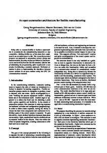
7.1 Maximum clock frequency of the router reported by the design compiler in pre-synthesis phase. . . . . . . . . . . . . . . . . . 109

xvi

List of Acronyms ACK Acknowledgement AES Advanced Encryption Standard ALU Arithmetic Logical Unit AR Access Router ASIC Application Specific Integrated Circuit AU Assembly Unit BB Basic Block BSV Bluespec System Verilog CE Compute Element CRC Cyclic Redundancy Check DFG data flow graph degree The degree of a router is defined as the number of links, it can establish to its neighbors and excludes the injection and ejection port. ECP Elliptic Curve Point ECPA Elliptic Curve Point (ECP) Addition ECPD Elliptic Curve Point (ECP) Doubling FIFO first-in-first-out flit A flit is the largest amount of data that can be transmitted between two routers in a clock cycle. The size of the flit depends on the amount of available wires laid out between the routers. HL HyperOp Launcher HyperOp Hyper Operation

xviii IHDF Inter HyperOp Data Forwarder IP Input Port IPC Intellectual Property Controller LIFO last-in-first-out LSU Load/Store Unit NoC Network on Chip OP Output Port PE Processing Element pHyperOp partial HyperOp radix The radix is the total amount of IPs and OPs a router can establish not only to its neighbors, but also to the attached units as well. Hence it includes also the injection and ejection port. RB Resource Binder SHA Secure Hash Algorithm SL Support Logic union A union in BSV is comparable with a union known in the programming language C. It can contain several structures such as packet structures, but only one is valid in any point in time. To distinguish which packet type is valid, the BSV compiler automatically add template bits according to the entries in the union. VC Virtual Channel VLSI Very Large Scale Integration

Chapter 1

Introduction In this chapter the evolvement of the Network on Chips (NoCs) originating from point-to-point connections and bus systems including the motivation for this work is described. After defining common terms that are used throughout this thesis, the reader will be exposed to a short introduction into Bluespec System Verilog (BSV) in which RECONNECT has been implemented.

1.1

Motivation

Within a chip, complex systems and multi-core architectures consist of many units called Processing Elements (PEs) that are either highly specific to perform a single task very efficiently, or comprise Arithmetic Logical Units (ALUs) for generic operations. The high level of integration of multiple (in an order of tens or even higher) PEs promise to satisfy the demand for computation power needed as of today. On the other hand these systems and architectures require a high speed communication system to exchange data among the PEs within the chip. One method is to analyze the traffic patterns of the executed application and building a communication system exactly matching these patterns by directly connecting the data exchanging PEs as shown in figure 1.1. While this point-to-point communication system is considered to be the fastest, it restricts the system designer to a few applications only. In addition depending on the richness of the system, the wiring requirements explode for n-to-n connections. A solution of this dilemma is rearranging the PEs to be connected via a cost efficient bus system, a shared resource in which only one PE can transmit data at a time. A control logic manages access granted to the bus. While this communication system gives the desired flexibility, it lacks scalability. In a magnitude of a thousand PEs which can be integrated easily in modern VLSI technology, the wires of the bus become very long and have a high capacitance resulting on long delays and high power consumption [39]. In the view of the allowed access of a single PE at a time, the throughput is

2

Introduction

PE

PE

PE PE

PE

PE PE

PE PE

Figure 1.1: A point-to-point connection always between a pair of PEs.

very low. Thus bus systems are only used, if a few tens of PEs need to communicate. To increase the utilization level bridges basically consisting of a set of first-in-first-out (FIFO) buffers, are inserted into the bus system, dividing the bus into several subsets (refer to figure 1.2a). If two PEs within a subset communicate, they can do so provided no other PE of the same group uses the bus at the same moment. With these bridges multiple PEs in different subsets are able to transmit data at the same time, since the bridges are opaque and the traffic cannot cross them. If the destination of the data resides in a subset outside of the current one, the bridge turns transparent and lets the traffic pass through it. If the bus consists of multiple bridges it can also be considered as a pipelined bus with each bridge representing one pipeline stage as shown in figure 1.2b. Each subset has its own arbitration control granting access to the bus segment either to one PE or to one bridge. However the time a message requires to cross the bus system from one side to the logically other, is immense. Depending on the amount of bridges and the size of the system, it can be in the order of thousands of clock cycles. In addition orchestration of the access to each subset and keeping track of the traffic crossing through several bus segments, increases the complexity in the global arbitration control. By rearranging the PEs into a more beneficial pattern such as a grid to cut short the long distances (refer to figure 1.2c), and by localizing the access control, the disadvantages of pipelined buses can be avoided. By now the access control not only regulates the grants to the shared bus resource, but also forwards the traffic into one of the multiple directions available.

1.1 Motivation

3

PE

PE

PE

PE

Control

PE

PE

PE

Control

(a) The bus is divided into two subsets separated by a bridge which is opaque, if the source and destination of a communication pair is within the same subset. Otherwise the bridge is transparent allowing the traffic to pass through it.

PE

Control

PE

PE

Control

PE

PE

Control

PE

Control

PE

PE

Control

PE

Control

PE

Control

PE

Control

PE

Control

PE

Control

(b) The bus is further divided by using more bridges.

(c) Rearrangement of the PEs to shorten the distances and decentralizing the access control logic.

Figure 1.2: A pipelined bus system

4

1.2

Introduction

Definition of commonly used Terms

The pattern in which the bridges and their connections among each other are arranged is henceforth called topology. The accumulation of the access control including the direction decision logic is called a router. Topology and routers form an Network on Chip (NoC). The NoC including the PEs among which the connectivity is established, is referred to as Fabric. An encapsulated piece of information outside the Fabric is called a packet. If it is inserted into the NoC, it is converted into a protocol that the router understands. This might include the necessity to divide the packet into several flits. Flits represent the largest amount of bits that can be transmitted at one instance of time between two routers. For instance a packet of a size of 80 bits is divided into 4 flits of 20 bits each. To transmit the flit, the connection between two routers need to consist of 20 wires at least. The number of connections that are established from one routers to all its neighbors, is referred to as degree. In figure 1.2c the routers located in the corners have a degree of two whereas the routers in the middle a degree of three. Usually the maximum degree only is given while listing the specifications of the NoC. The degree depends on the topology that a router is integrated into, and it differs from the term radix, which represents the total number of connections a router provides including the links to all connected PEs. Again referring to the same figure the radix of the corner router is three whereas the radix of the routers in the middle is four. Assuming each router has 4 PEs connected to it, the radix becomes 7 and 8 respectively. Besides the characteristics for a router, the NoC can be described by the bisection bandwidth which is obtained by dividing the network into two disjoint sets of nearly equal size. The partition with the lowest number of connections originating in one set and ending in the other one, determines the bisection bandwidth. For the system designer deciding on the topology, it is important to know the maximum number of hops a flit has to travel to the source and destination that are farthest apart. This characteristic is called diameter of the network. Table 1.1 compares these characteristics in an overview. The time a flit traverses through the network is referred to as latency. Usually system designers are interested not only when the flit arrives, but also when the packet consisting of multiple flits, is ejected from the network and available for processing. Hence the latency also includes the time needed for segmentation and reassembly of the packet (serialization latency). The higher the number of flits and hence the higher the network load, the higher is the latency due to the occurrence of congestions, in which flits have to share a common path. The network load can reach a point in which the throughput saturates. If the saturation point has been reached, the router does not always accept injected packets anymore and these packets need to be queued. Throughput depends on the underlaying topology, the clock

1.3 A short Introduction into Bluespec System Verilog (BSV)

5

Table 1.1: Properties of commonly used topologies

Topology Mesh Honeycomb Honeycomb (rectangular) Hexagonal Hexagonal (rectangular) Toroidal Topologies Mesh Honeycomb Honeycomb (rectangular) Hexagonal Hexagonal (rectangular) Hypercube

Degree (deg) 4 3 3 6 6 4 3 3 6 6 log n

Diameter (dia) √ 2 n √ 1.16 n √ 2 n √ 1.16 n √ 2 n √

n √ 0.81 n √ n √ 0.58 n √ n log n

Bisection Bandwidth √ n √ 0.82 n √ 0.5 n √ 2.31 n √ 2 n−1 √ 2 n √ 2.04 n √ n √ 4.61 n √ 4 n−2 0.5 × n

frequency of the router and the flit size.

1.3

A short Introduction into Bluespec System Verilog (BSV)

RECONNECT is implemented in the high-level language BSV [6, 12, 11] which allows to compile it into a clock accurate simulator that can be executed on ordinary end user PCs, but also to compile it into Verilog files for further processing by e.g. synthesis tools. By using one code for simulation and synthesis, code maintenance is minimized, since consistency does not need to be ensured among several implementations. In addition BSV allows to use certain constructs which are hard to understand for developers coming from hardware design background, but are well known to software programmers. On the other hand many times the software programmer lacks the experience and knowledge of hardware programming. As an example, if b=a×4+3

(1.1)

needs to be calculated, a software developer will most likely write the equation directly into the program. However the hardware engineer knows that the multiplication is a simply shift of a by 2 bits to the left and the addition by 3 means that the last 2 bits of b are set after assignment of a to b. Equation 1.1 is equivalent to b = (a = 2 i f ( dir == SOUTH ) { i f ( dx == 0 && dy == 0) opNo = EJECT ; e l s e opNo = EAST ; } i f ( dir == WEST ) { i f ( dx == 0 && dy == 0) opNo = EJECT ; else { i f ( dy > 0) opNo = SOUTH ; e l s e i f ( dy < 0) opNo = NORTH ; e l s e opNo = EAST ; } }

61 62 63 64 65 66 67 68 69 70 71 72 73 74 75

i f ( dir == NORTH ) { i f ( dx == 0 && dy == 0) opNo = EJECT ; else { i f ( dx > dy * (−1) ) opNo = EAST ; e l s e opNo = WEST ; } }

76 77 78 79 80 81 82 83

i f ( dir == EAST ) { i f ( dx == 0 && dy == 0) opNo = EJECT ; else { i f ( dy > 0) opNo = SOUTH ; e l s e opNo = WEST ; } }

84 85 86 87 88 89 90

} return opNo ;

91 92 93

} Listing 4.1: Full rule set defining where flits need to be forwarded to depending on the relative address, the location of the IP, the VC and if the router has a port to the north.

55

56

Routing Algorithms (Routing(.*).bsv) and Topologies

This information has been obtained by merely observing, what directions are allowed. If there is only one outgoing port (for instance a flit in VC0 in the IP located in the SOUTH, cannot be routed to the east), the necessary action is obvious and the port should include only one possible outgoing direction. Since the algorithm consists of multiple layers, the eastern direction is only allowed, if the VC number is changed as done in line 9. The flit changes into another VC, if it reaches the diagonal. This can only happen, if flit is traversed the NoC in a step like pattern and is stored in the southern buffer of the node on the diagonal. 4.4.1.2 if Branch Aggregation As a first step of optimization conditions which are common for all if branches, are aggregated. For instance almost all branches include the condition for the ejection port. The only branch that does not include a condition for ejection, is the injection port itself. It is assumed that no flit is sent back into the same direction where it just came from. Hence it is safe to include the ejection as a condition into the injection port. As it can be observed further is the similarity of the appropriate if branches. For instance the conditions for the northern IP are the same regardless the VC number a flit is currently residing. Listing 4.2 shows the result of the routing algorithm after the first optimization step. 1

2

direction routingHoneycomb2D_VC ( i n t dx , i n t dy , i n t * vcNo ←, const bool northPort , const direction dir ) { direction opNo = INVALID ;

3 4 5 6 7 8 9 10 11 12 13

i f ( dx == 0 && dy == 0) opNo = EJECT ; else { i f ( dir == SOUTH ) { i f ( * vcNo == 0) { i f ( dx >= dy * (−1) ) { i f ( * vcNo 0) opNo = SOUTH ; e l s e opNo = EAST ; } else { i f ( dy > 0) opNo = SOUTH ; e l s e i f ( dy < 0) opNo = NORTH ; e l s e opNo = EAST ; }

4.4 Honeycomb Topology } i f ( dir == NORTH ) { i f ( dx > dy * (−1) ) opNo = EAST ; e l s e opNo = WEST ; }

24 25 26 27 28 29

i f ( dir == EAST ) { i f ( * vcNo == 0) { i f ( northPort ) { i f ( dy < 0) opNo = NORTH ; e l s e opNo = WEST ; } else { i f ( dy > 0) opNo = SOUTH ; e l s e opNo = WEST ; } } else { i f ( dy > 0) opNo = SOUTH ; e l s e opNo = WEST ; } }

30 31 32 33 34 35 36 37 38 39 40 41 42 43 44

i f ( dir == INJECT ) { i f ( northPort ) { i f ( dy < 0) opNo = NORTH ; e l s e i f ( dy > 0) { i f ( dx < 0 && abs ( dx ) >= dy ) { i f ( * vcNo 0) opNo = EAST ; e l s e i f ( dx < 0) opNo = WEST ; } } else { i f ( dy > 0) opNo = SOUTH ; e l s e i f ( dx >= dy * (−1) ) { i f ( * vcNo = dy*(-1) is true. Only if the diagonal has not been reached, the flit stays in its VC and is routed to the west as long as the diagonal or the destination is reached. In that case the condition dx >= dy*(-1) is false and the VC is not changed. In the eastern port a flit in VC2 is either forwarded to the west or south whereas a flit in VC0 is sent either north, south or continues to the west. Since the turn east to north is prohibited in VC2, we have to check, if the situation can occur in the first place before removing the VC condition. A flit that is in VC2 of the eastern port and wants to go to north, is sent to this router by the previous router with a southern port. In the latter router the flit could have come from the east or south. 1. If it had come from the east, a change to VC2 would have had occurred only if it had come from the north in the previous router. But since flits do not go back into the same direction, this situation is impossible. 2. It cannot come from the south, because the turn south to west is prohibited in VC2. So a flit residing in VC2 of the eastern port, and which wants to go to the north, does not exist.

4.4 Honeycomb Topology

59

The optimizations result in a VC independent routing algorithm as shown in listing 4.3. 1

2

direction routingHoneycomb2D_VC ( i n t dx , i n t dy , i n t * vcNo ←, const bool northPort , const direction dir ) { direction opNo = INVALID ;

3 4 5 6 7 8 9 10 11 12 13 14 15 16 17 18 19 20 21 22 23 24 25 26 27 28 29 30 31 32 33 34 35 36 37 38 39 40 41 42 43 44 45

i f ( dx == 0 && dy == 0) opNo = EJECT ; else { i f ( dir == SOUTH ) { i f ( dx >= dy * (−1) ) { i f ( * vcNo 0) opNo = SOUTH ; e l s e i f ( dy < 0) opNo = NORTH ; e l s e opNo = EAST ; } i f ( dir == NORTH ) { i f ( dx > dy * (−1) ) opNo = EAST ; e l s e opNo = WEST ; } i f ( dir == EAST ) { i f ( northPort ) { i f ( dy < 0) opNo = NORTH ; e l s e opNo = WEST ; } else { i f ( dy > 0) opNo = SOUTH ; e l s e opNo = WEST ; } } i f ( dir == INJECT ) { i f ( northPort ) { i f ( dy < 0) opNo = NORTH ; e l s e i f ( dy > 0) { i f ( dx >= dy * (−1) ) opNo = EAST ; else { * vcNo = 2 ; opNo = WEST ; } } else { i f ( dx > 0) opNo = EAST ; e l s e i f ( dx < 0) opNo = WEST ; } } else { i f ( dy > 0) opNo = SOUTH ; e l s e i f ( dx >= dy * (−1) ) {

60

Routing Algorithms (Routing(.*).bsv) and Topologies i f ( * vcNo = 0) temp = 0 ; dx += temp ; dy += temp ; dz = temp ;

4 5 6 7 8 9 10 11

} Listing 4.7: The conversion algorithm to convert a two tupled address into a three tupled one

4.6 Hexagonal Topology

4.6.1

65

Proof

The algorithm converts a relative 2D address into a relative 3D address so that the flit traverses on the shortest path. In 2D addressing nine possibilities of how the tuple can look, exist like as there are: (+, +), (+, −), (−, +), (−, −), (0, +), (+, −), (+, 0), (−, 0), and (0, 0). • In case the tuple is (+, +) (line 4), dz(a) is not going to be 0. Instead it is the complement of the lower value of dx(a) or dy(a) and hence negative. Since dz(a) will either be equal to −dx(a) or −dy(a) one or both are nullified meeting the requirement of the shortest path routing. • Similar if the tuple is in the format (−, −) (bypassing the if and else branch). In that case, dz(a) is positive and similar to the reasoning above one or both components of the 2D address will be set to 0 in the addition sequence starting in line 9. If e.g. dy(a) < dx(a) < 0, the result will be:

dynew (a) = dyold (a) + dxold (a),

(4.1)

since dyold (a) < dxold (a) ⇒ dynew (a) < 0 dxnew (a) = dxold (a) + |dxold (a)|,

(4.2)

with dxold (a) < 0 ⇒ dxnew (a) = 0 dznew (a) = |dxold (a)| > 0

(4.3)

In both cases the route that a flit takes without conversion will be an L shape in figure 4.12 and it can be observed that by introducing a path parallel to the z axis, the way can be cut short. E.g. consider the route from P to O. Instead of traveling the route (1, 2) which comprises of 3 hops, the original relative address is (0, 1, −1), resulting in 2 hops. • All other cases are handled by the else if branch in line 6. If one of the 2D address elements is equal or greater than 0, the other one needs to be either equal to 0 ((0, 0), (+, 0), (0, +)) or is less than 0 ((+, −), (−, +), (0, −), (−, 0)), because the case of (+, +) has already been handled by the earlier if condition. In this situation the flit is either traversing in parallel to one of the x or y axis (if one of the component of the 2D address is equal to 0) or the z component is counterproductive and does not help in finding a shorter path. Hence dz(a) is set to 0 meeting again the requirement of the shortest path routing. To avoid deadlocks the routing algorithm in [62] can be described as a negative-first algorithm. If it is taken under consideration that there is at

66

Routing Algorithms (Routing(.*).bsv) and Topologies

maximum only one negative component in the 3D address tuple, since one of the remaining elements must be either positive, if the last one is 0, or both are equal to 0, a simplified priority based algorithm can be used checking first for the negative address tuples. Such an algorithm is given in listing 4.8. 1

direction getRouteHexa_NegFirstnoVC ( i n t dx , i n t dy , i n t dz ) {

←-

2

i f ( dx == 0 && dy == 0 && dz == 0) return EJECTPORT ;

3 4 5

i f ( dx < 0) return i f ( dy < 0) return i f ( dz < 0) return i f ( dx > 0) return i f ( dy > 0) return return NORTHWEST ;

6 7 8 9 10 11 12

WEST ; NORTHEAST ; SOUTHEAST ; EAST ; SOUTHWEST ; // f o r dz > 0

}

13 14

15

16 17 18

direction getRouteHexaDateLine_NegFirst2DVC ( direction dir ←[ 3 ] , i n t dx , i n t dy , i n t dz , i n t &vc ) { direction nextOutput = getRouteHexa_NegFirstnoVC ( dx , ←dy , dz ) ; i f ( nextOutput == in_array ( dir ) ) vc++; return nextOutput ; } Listing 4.8: The negative-first routing algorithm in hexagonal topologies.

4.7

Summary

In this chapter the routing algorithm for three topologies (honeycomb, mesh and hexagonal) has been described. In addition other topologies of potential interest such as the Flattened Butterfly, Spidergon and Stargon topologies have been introduced. By using a step-by-step explanation method, the system designer is able to develop new routing algorithms for other topologies as well. The algorithms are tightly connected to the chosen topology. Currently RECONNECT supports the three topologies mentioned earlier at the same time by superimposing the honeycomb onto a mesh and further the mesh onto the hexagonal topology. Again the system designer has the freedom to tailor RECONNECT to be integrated into one only or into a new topology such as a ring by disabling additional IP/OP pairs.

Chapter 5

Test Case: REDEFINE The architecture in which RECONNECT is integrated is called REDEFINE, a dataflow oriented, reconfigurable multi-processor architecture (refer to [57]). It consists of supporting logic (refer to section 5.2) and a portion performing the computation called Fabric as described in section 5.3. The Fabric comprises multiple tiles and an interconnect realized by a Network on Chip (NoC). Each tile consists of an NoC router and a Compute Element (CE) which is equivalent to a computation core in modern personal computers. Depending on the requirement and which algorithm is executed on REDEFINE, CEs can be replaced by specialized ones with extra functionality provided by added or replaced modules in the Arithmetic Logical Unit (ALU). Hence the Fabric becomes heterogeneous, if requirements dictate. A data flow processor is a processor lacking a program counter stating the next instruction to be executed. Instead instructions and their operands are marked as ready, if all operands have arrived. After readiness has been achieved, the instructions are scheduled to be executed. Hence the order of execution is not determined which results in a higher utilization of the ALU due to the avoidance of delays for completion of load and store instructions. In real cases however memory dependencies must be respected such as in the example listing 5.1. 1 2 3 4 5

a = b + c; i f ( a > 10) d = 2 * a; else d = d 4 occur although the maximum distance from any source to any destination cannot be more than three hops (refer to figure 5.10). The SL is not yet aware of the vertical toroidal links and is not utilizing them. Although the average hop count is already very low, it is expected to decrease further, once the SL supports all toroidal links. The additional links of Flattened Butterfly bypassing immediate neighbors will not be utilized very often. As described in chapter 7 every Input Port (IP)/Output Port (OP) pair contributes significantly to the area and power consumption. Taking the router with a radix of four as a basis to perform the power and area calculations, each IP/OP pair adds approximately 25% and 50% to the area and power consumption respectively. According to these numbers, a router with a low radix would be preferable. Thus the implementation of this kind of topology cannot be justified.

−1

0

1

2

3

−2

−1 0 1 2 3 −2 Figure 5.10: The row and column wise distances of nodes as seen from the black one. In a toroidal 6 × 6 Fabric the distances for each dimension cannot exceed three hops.

Although not contributing significantly to the average, for many applications it can be observed that there are exactly 6 flits be routed in x-direction with a hop count ≥ 2 such as in LU or MATMUL. These are the configuration packets determining the topology that is desired. The packets do not affect the overall execution time as mentioned in section 5.4 on page 73. Since these packets are injected into the NoC well before any application can be launched, it is irrelevant, how many hops they travel and therefore how long it takes to forward them to their destinations.

5.5.6

Spidergon and Stargon Topology

Unfortunately neither the Spidergon nor the Stargon topology described in section 4.2.2, are suitable for REDEFINE in which specifications state that HyperOps can occupy a 5 × 5 section of the Fabric at maximum. Spidergon is too small with 4 × n with n > 0 nodes and is hence not a solution.

84

Test Case: REDEFINE

Regarding the Stargon topology as shown in figure 4.4d on page 46, it can be observed that the NoC is divided into two layers of the same size (shaded in the figure) connected by a few extremely long links. The upper half can communicate with the lower half only through these links. While the largest HyperOp can be supported by this topology, a heavy penalty is expected to be paid, if the HyperOp is spread over the two halves. As an alternative, the NoC can be resized to such an extent that each half can accommodate the largest HyperOp. But this makes it necessary to create a 10 × n with n > 5 topology. Any HyperOp that does not have any input values or whose input values coming from executing HyperOps have arrived, are ready to be launched. In case of an application in which the HyperOps are very small or have a high dependency among them and hence have to be launched sequentially, a larger NoC results in many unused resources. Hence a Stargon topology seems also to be unpractical for REDEFINE. The main problem is that the logical structure of both topologies with the nodes at the boundaries of the network, does not match the two dimensional arrangement of nodes expected by the SL of REDEFINE. Hence these topologies are not further investigated.

5.6

Summary

To obtain numbers about the performance of RECONNECT, it has been integrated into a target architecture called REDEFINE which is briefly described. In this case the performance measurement was the Fabric Execution Time which stated how long an execution took in various configurations. One take away from this exercise is the finding that the topology of an NoC cannot be considered completely independent of the target architecture. The SL of REDEFINE is not aware of the used topology. Hence the expectations of providing a richer topology such as the hexagonal one, could not be met: The execution time of applications did not decrease significantly. By analyzing the traffic pattern it can be concluded that the Flattened Butterfly as well as Spidergon and Stargon topologies are not an option for REDEFINE at the moment. The additional links of the Flattened Butterfly will be hardly utilized. In case of Spidergon and Stargon the support logic and the way applications are mapped onto the Fabric, make any potential benefits offered by these topologies, negligible.

Chapter 6

Artificial Traffic Generators To obtain essential characteristics such as latency and throughput of RECONNECT, the Processing Elements (PEs) have been replaced by artificial traffic generators inducing different kind of traffic patterns into the Network on Chip (NoC). In this chapter the test environments and used generators are described in details. Beside a traffic generator injecting traffic uniformly, also self-similar traffic traces have been generated. Apart from these different traffic patterns, the destination address of the flit plays a significant role. Each traffic generator is divided into four categories: 1. Normal: The address range is only limited by the size of the NoC. In a 6 × 6 toroidal NoC such as the one in REDEFINE, a tuple of the relative address ranges from −2 to 3 in each direction to reach any destination from any source. 2. Close Neighbor: All packets are destined to the immediate neighbors. This setting restricts the relative address to range from −1 to 1 in each direction. 3. Bit Complement: The absolute address of the destination is calculated by bit complementing each coordinate of the source address. This result in a star like pattern in which the flits are send diagonally across the network. 4. Tornado: In a 6 × 6 Fabric the relative destination tuples always equals (2,2). Hence toroidal links are as any other link heavily included in this configuration. Formally each tuple of the address is calculated by

addrdest = addrsrc + (dn/2e − 1)

mod n

in which n equals the number of nodes in a direction [17].

(6.1)

86

6.1

Artificial Traffic Generators

Test Environment

The traffic generator determines at what time a flit with what address needs to be injected into the network. If the router does not accept the flit at the specified time, the flit needs to be queued. This queue needs to be empty and all flits must have arrived at their destinations, before the test can be concluded. While the flit waits in the queue for its turn, its latency count increases with every clock cycle. Each test run has a warm-up phase in which flits are injected into the network, but do not contribute to the measurement of the overall performance. In the conducted tests a warm-up phase of 1000 clock cycles was used. After the test, which was executed for 1000000 cycles, a cool down phase started, in which the traffic generators were deactivated to allow the built up queues to be flushed into the NoC.

6.2

Uniform Traffic Pattern

A artificial generator for uniform traffic can randomly create a flit at any point in time. It depends on only a single threshold value stating how often and at what time a flit is injected. With that value, the offered load can be controlled. Figure 6.1 and figure 6.2 display the latency and throughput in term of maximum capacity of the network for various offered loads respectively. The latency results obtained are comparable with the numbers presented in [34] and justify this approach and test environment. As it can be observed, the throughput for close neighbor communication is significantly higher, if compared with the normal address generation method. This is expected, since the flits are ejected from the NoC at a very early stage. Interestingly the throughput does not always increase, if the offered load is intensified (refer to figures 6.2a and 6.2d). This is due to the so called weak fairness of the arbiters. Since they do not consider the age of the flit due to the reasons elaborated in 3.3.2.1, flits competing for common resources might stay an unequal amount of time in the Virtual Channels (VCs). Comparatively old flits are not assigned a higher priority than freshly arriving flits. Consider the following example: A flit A that already waits for a long time in a VC, but could not be forwarded due to unavailability of the receiving VC of the next router. A new flit B arrives in another VC for the same destination like flit A and at the same time the receiving VC becomes available. In case that the VC in which flit A resides has been served last by the VC arbiter, it will grant the resources to flit B instead, resulting that flit A waits even longer. By using the crossbar comprised of muxes and demuxes only, RECONNECT routers can be configured to require only one single clock cycle to forward flits. Without raising the level of complexity of the arbiters located in the critical path of that single cycled router, this problem of the weak fairness

6.2 Uniform Traffic Pattern

87

cannot be addressed. Since the load on the network is very low for the applications mentioned earlier, so that congestions hardly occur, the decrease of throughput for loads beyond 30% to 40% is acceptable. In addition, since during the execution of the applications mostly very close neighborhood communication is encountered, the problem of unfair arbiters does not occur.

88


50

Honeycomb Mesh Hexagonal

Latency [Cycles]

40 30 20 10 0 0.1

0.2

0.3 0.4 Offered Load

0.5

0.6

(a) Normal

50


Latency [Cycles]

40 30 20 10 0 0.1

0.2

0.3

0.4 0.5 0.6 Offered Load

0.7

0.8

(b) Close Neighbor

Figure 6.1: Latency for uniform traffic patterns and various address generation methods

0.9


89

50


Latency [Cycles]

40 30 20 10 0 0.1

0.15

0.2

0.25 0.3 Offered Load

0.35

0.4

(c) Tornado

50


Latency [Cycles]

40 30 20 10 0

0.1 0.12 0.14 0.16 0.18 0.2 0.22 0.24 0.26 0.28 0.3 Offered Load (d) Bit Complement

Figure 6.1: Latency for uniform traffic patterns and various address generation methods


Throughput [% of Network Capacity]

90

50


45 40 35 30 25 20 15 10 5 0.1

0.2

0.3

0.4


0.8

0.9

1

0.9

1


(a) Normal

90


80 70 60 50 40 30 20 10 0 0.1

0.2

0.3

0.4


0.8

(b) Close Neighbor Communication

Figure 6.2: Throughput for uniform traffic patterns and various address generation methods



91

50


45 40 35 30 25 20 15 10 5 0.1

0.2

0.3

0.4


0.8

0.9

1

0.9

1


(c) Tornado

35


30 25 20 15 10 5 0.1

0.2

0.3

0.4


0.8

(d) Bit Complement

Figure 6.2: Throughput for uniform traffic patterns and various address generation methods

92

6.3


Self Similar Traffic Pattern

In real life situations it can be observed that the traffic is not uniformly randomly distributed. Instead it has a bursty character in which in a very short time period a comparatively large amount of data is transmitted, followed by duration in which no flit is generated at all [47]. Hence the traffic generator has been extended to accommodate these characteristics. The generator has two states: One in which the generator is deactivated and in off-state. In on-state the generator injects flits according to the configured injection rate. The generator remains in on-state and off-state for ton and tof f cycles respectively as given below: −1

ton = (1 − r) αon tof f = (1 − r)

−1 αof f

(6.2) (6.3)

r is a random variable uniformly distributed between 0 and 1. αon and αof f have been fixed to 1.9 and 1.25 respectively [7]. The latency and throughput results of self similar traffic patterns are depicted in the figures 6.3 and 6.4 respectively. These results are not comparable with the ones given in section 6.2. While in uniform traffic pattern the traffic generator stays always in an active state and hence continuously injects flits according to the injection rate, it is not the case in self similar traffic generators. There are periods in which the generator is deactivated, hence by the end of the simulation the number of injected flits is lower. Another testing method would be to adapt the injection rate. The longer the generator is deactivated, the higher must be the injection rate while it is active. It would be useful to validate this approach against results in published literature such as [27]. However the exact testing environments are not described, hence making it difficult to compare.

6.3 Self Similar Traffic Pattern

93

50


Latency [Cycles]

40 30 20 10 0 0.1

0.2

0.3

0.4


0.8

0.9

1

0.9

1

(a) Normal

50


Latency [Cycles]

40 30 20 10 0 0.1

0.2

0.3

0.4


0.8

(b) Close Neighbor

Figure 6.3: Latency for self similar traffic patterns and various address generation methods

94


50


Latency [Cycles]

40 30 20 10 0 0.1

0.2

0.3

0.4


0.8

0.9

1

(c) Tornado

50


Latency [Cycles]

40 30 20 10 0 0.1

0.2

0.3


0.7

0.8

(d) Bit Complement

Figure 6.3: Latency for self similar traffic patterns and various address generation methods

0.9


6.3 Self Similar Traffic Pattern

95

35


30 25 20 15 10 5 0 0.1

0.2

0.3

0.4


0.8

0.9

1

0.9

1


(a) Normal

35


30 25 20 15 10 5 0 0.1

0.2

0.3

0.4


0.8

(b) Close Neighbor Communication

Figure 6.4: Throughput for self similar traffic patterns and various address generation methods



96

35


30 25 20 15 10 5 0 0.1

0.2

0.3

0.4


0.8

0.9

1

0.9

1


(c) Tornado

30


25 20 15 10 5 0 0.1

0.2

0.3

0.4


0.8

(d) Bit Complement

Figure 6.4: Throughput for self similar traffic patterns and various address generation methods

6.4 Summary

6.4

97

Summary

In this chapter the traffic generators and the testing environment have been described in detail. It could be observed that the weak fairness of the arbitration stages causes a drop in throughput after reaching a peak at an offered load of 30%. As expected the throughput increases, the richer the network is. Thus the hexagonal topology shows the highest performance followed by the mesh topology. The honeycomb topology gives the worst results. The obtained results are comparable with the ones found in literature such as [34]. However in some publications the tabulated performances are much better. Unfortunately in many cases the test environments are not described detailed enough to allow comparisons or to draw any conclusions. For instance another method apart from the one described in this chapter, would be that the flit is dropped, if the router does not accept it at the specified time due to congestions. Hence the average latency is not increased by waiting flits. In the end the number of flits that are injected into the network, is lesser compared to the number of flits injected by using a queue, although the injection rate is the same from the point of view of a generator. The take away from the exercise in this chapter is that, if a paper is published promising to improve the performance, the ideas need to be implemented and run against the own test traffic patterns before conclusions can be drawn.

98


Chapter 7

Synthesis Results A router including its assembly unit has been synthesized by using Design Vision and FSD0A_A 90nm standard cell library for UMC’s 90nm logic SP-RVT (Low-K) for typical cases for different flit sizes of interest. As mentioned before only sizes which cause packets to be segmented into different flits and have the minimum of unused bit are analyzed (refer to figure 5.4) to obtain power and area details. For NoC routers realistic power number are difficult to acquire. One reason is the availability of various methods of measurement as described below. Another reason is that from a global point of view the routers of the network are in different states and busy levels. If the CRC application (section 5.5.1) is considered as an example, it can be observed that in a Fabric of 6 × 6 nodes, only 3, at maximum 4 nodes depending on the configured topology, are used. The other nodes and their routers remain idle, not consuming any switching power. In this section a single router has been analyzed while the activity factor has been fixed to 0.5 which reflects a switching of every clock cycle and is therefore the worst power consumption. Mainly two different measurement methods exist, if power and area numbers need to be acquired: 1. The router including the Assembly Unit (AU) is synthesized, but the ports are left unconnected. The synthesis tool can induce the activity factor only on those ports which are exported through interfaces. However for estimations about the area consumption, these ports are optimized to the extent that they become non-existent. To prevent this undesired optimization the Input Ports (IPs) and Output Ports (OPs) can be connected to buffers. However before a flit can be stored in the VC, the previously calculated VC is read from the head flit and after which the flit is stored in the appropriate VC. If the ports are left unconnected, these logical blocks do not count for the critical path calculation which is the longest path between two buffers and hence determines at which clock frequencies a circuit is able to operate.

100

Synthesis Results Neglecting this issue results in wrong estimates about the maximum frequency.

2. To avoid the removal of the unconnected IPs and OPs, the OPs are connected to the IPs in the second measurement method. However since the IP and OP interfaces are no longer exposed, the tool cannot induce an activity factor into these ports. The only interface that is left unconnected is the one towards the sink/generator. While this gives certainly lower power numbers compared to the first method described above, the area numbers and the estimate about the maximum clock frequency are more realistic, since the complete length of the path a flit has to travel from its buffer to the receiving buffer is considered.

7.1

Synthesis Tool Parameters

The following numbers have been obtained by the Synopsis tool “Design Vision” and are an estimation. Accurate power and area numbers can only obtained after post synthesis which is not done in this work, since REDEFINE itself needs to mature, before this step can be taken. The following parameters are set, if not mentioned otherwise: • A clock frequency of 450MHz corresponding to the master clock given to REDEFINE. • Each IP consists of four VCs and each VC is a first-in-first-out (FIFO) buffer capable of holding four flits in total. • The AU is included in the router. • Relative addressing scheme so that the OP needs to update the header flit every hop. • Activity factor of 50%. • It is unlikely that the support for multiple topologies provided by the router, will be utilized once RECONNECT is integrated into a target architecture. Thus for each hexagonal, mesh and honeycomb topology a router configuration has been compiled into Verilog. Further several configurations with various flit sizes have also been created and compiled for each one of the topologies.

7.2 Area and Power Consumption of the Single Cycle Router

7.2

101

Area and Power Consumption of the Single Cycle Router

As can be observed in figure 7.1, the rate of power as well as the area consumption between the smallest (20 bit) and the largest flit (116 bit), is almost linear with the flit size for all topologies. At 115 bit the highest power consumption is observed, even more than at 116 bit of flit size. The reason is that at a flit size of 116 bit, the AU becomes obsolete, since packets do not have to be segmented into multiple flits any more, which in turn leads to a lower overall power consumption of the router. In mesh topology the router has an additional port activated when compared to honeycomb. From figure 7.1a an estimate can be derived of how much power each added and active port consumes. Depending on the flit size a router integrated in a mesh topology consumes approximately 27% to 30% more power when compared with a router in a honeycomb topology. Hexagonal routers need around 48% more power than routers in mesh. This number is doubled, if the hexagonal router is compared with one that is integrated in a honeycomb topology. As a rule of thumb, it can be said, that each IP/OP pair added to the honeycomb router, increases the power consumption by approximately 25%. It is obvious that with additional ports, also the area required by the router increases (refer to figure 7.1b). Like the power consumption, the area increases linearly with the flit size. A router integrated in a mesh topology requires between 26% and 30% more area than a router in a honeycomb topology depending on the flit size, whereas a router in hexagonal topologies approximately 50% and 91% more than a router in a mesh and honeycomb respectively. The linear increase of power and area with the increase of the flit size suggests that the router does hardly have control logic which depends on the flit size. Roughly speaking the control logic comprises of: • Routing algorithm, • VC arbitration within the IP, • OP arbitration for competing IPs, • and relative address update mechanism. The main purpose of a router is to transfer data from one port to another one. Hence it mainly consists of buffers and buses which hugely depend on the size of a flit. For instance the VCs have registers which allow to store several flits. If the flit size is changed, so are the registers resulting in a removal or addition of registers. The same applies to all buses that a flit encounters while traversing through the modules of the router. Hence the

102

Synthesis Results

80 Hexagonal Mesh Honeycomb 70

Power Dissipation [mW]

60

50

40

30

20

10 20

30

40

50

60

70 80 Flit Size [Bits]

90

100

110

120

90

100

110

120

(a) Power 7 Hexagonal Mesh Honeycomb 6

Area [105 Cells]

5

4

3

2

1

0 20

30

40

50

60


(b) Area

Figure 7.1: Power and area consumption of a single router for various flit sizes. The drop at 116 bit is caused by the removal of the AU whose functionality of segmenting packets into multiple flits is not required at these sizes anymore.

7.3 VC Depth

103

gate count is approximately linear with the flit size and since the gate count is proportional to the area consumption, the area is also expected to change linearly.

7.3

VC Depth

During the execution of applications described in section 5.5 it was observed that the VCs hardly reach a state in which they do not accept any data anymore. Even congestions and competitions of several IPs for a single OP as the ones described in section 5.5.3 are resolved quickly. Hence it can be assumed that the VCs can be reduced to a depth in which they can hold the largest packet completely comprising of multiple flits which is:

VCDepth

L = B

(7.1)

with B being the flit size and L representing the maximum packet size, which is currently 116 bits in case of REDEFINE. Figure 7.2 depicts the power and area consumption with the newly adapted VC depths. As it can be observed, a reduction of flit size does not necessarily result in a lower area and power consumption. If, for instance, the flit size is reduced from 76 to 57 bits, the largest packet needs 3 flits in total to accommodate its payload. Hence the depth of the VC is increased by one flit. In total it is possible to store 3 × 57 = 171 bits in total for each VC, whereas it was only 2 × 76 = 152 bits in the previous case. At flit sizes of 116 bits all VC depths are reduced to one since the flit size corresponds to the packet size exactly. Compared to the power and area ratings discussed in section 7 the increase is moderate, when the flit size is enlarged. In fact a router supporting a flit size of 76 bits has nearly the same power and area consumption when compared with a flit size of 43 bits. With this finding and in view of the Fabric Execution Time (refer to section 5.5 for various applications), it seems unreasonable to use routers supporting only the smaller flit sizes causing a drastic increases of the execution time. Regarding the chosen flit sizes: As mentioned in section 5.5.1 only those flit sizes are investigated, at which the number of flits for a given set of packets differs and the number of unused flits is minimal (refer to figure 5.4).

104

Synthesis Results

55 Hexagonal Mesh Honeycomb

50


45 40 35 30 25 20 15 10 20

30

40

50

60


90

100

110

120

90

100

110

120

(a) Power 4 Hexagonal Mesh Honeycomb 3.5

Area [105 Cells]

3

2.5

2

1.5

1 20

30

40

50

60


(b) Area

Figure 7.2: Power and area consumption, if the VC has to hold one packet eventually comprising of multiple flits.

7.4 Area and Power Consumption of the Pipelined Routers

7.4

105

Area and Power Consumption of the Pipelined Routers

As mentioned in section 3.6 the currently provided throughput is not sufficient for various application such as in H.264 decoding. At a clock speed of 450MHz and a flit size of 116 bits, the gross throughput per link peaks at 6.07GBps including information for control such as addressing and VC calculations. Since the wiring complexity is high, a more realistic bus width between the routers will be 32 or 64 bit [61, 49] after deduction of the control field to match the available payload field the word length of the attached processing cores. In addition the link throughput does not consider congestions, if e.g. multiple modules of the H.264 access the same shared memory provided by the Load/Store Unit (LSU). Based on the results of the artificial traffic generators (refer to section 6) and under the assumption that a mesh topology is used for implementing a H.264 decoder, the network has to provide four times (see below) the capacity to forward the flits in time which is limited by the frame rate of the video stream. If a flit carries 4 Bytes payload and if a bandwidth between memory and processing core needs to be 637MBps, the router needs to forward 166, 985, 728 flits per second. Due to the saturation point of the mesh topology at approximately 25% of network capacity (refer to figures 6.1a and 6.2a), the router should be able to process 166, 985, 728 × 4 = 667, 942, 912 flits. Even if the router operates at the maximum frequency of 550MHz, it can forward only 550, 000, 000 flits on a single link per second at maximum. Since this peak performance is a theoretical value and it is most unlikely to be reached in reality, is it obvious that this throughput cannot be accomplished with the current implementation, justifying engineering efforts for a pipelined version. As mentioned earlier in section 3.6.1, there are two pipelined versions available: 1. One pipeline stage after IP/OP arbitration (version 1). 2. In version 2 the crossbar establishing the connectivity between each IP to all OPs of a router, is replaced by a butterfly crossbar providing three pipeline stages in total (refer to figure 3.8 on page 35). This implementation does not require an IP/OP arbitration. Whereas in the first version the area consumption and power dissipation is almost equivalent with the results that are presented for the single cycle router, since only 24 (honeycomb topology) to 49 (hexagonal topology) flip flops are needed additionally to retain the states of the arbiters, a tremendous increase in both area and power can be observed in the router using the pipelined butterfly crossbar. This is due to the drastic increase of required

106

Synthesis Results

storage capacity in the pipeline stages. Figures 7.3 and 7.3b depict the area and power consumption of the router respectively. To allow a fair comparison, all settings such as activity factor and frequency, remain the same.

7.4 Area and Power Consumption of the Pipelined Routers

107

350 Hexagonal Mesh Honeycomb


300

250

200

150

100

50 20

30

40

50

60


90

100

110

120

90

100

110

120

(a) Power 14 Hexagonal Mesh Honeycomb 12

Area [105 Cells]

10

8

6

4

2 20

30

40

50

60


(b) Area

Figure 7.3: Power and area consumption of a single pipelined router using a butterfly as a crossbar for various flit sizes. The drop at 116 bit is caused by the removal of the AU whose functionality of segmenting packets into multiple flits is not required at these sizes anymore.

108

7.5

Synthesis Results

Maximum Clock Frequency

The maximum frequency is calculated from the maximum path length between two buffers including their hold and setup time. The impact of the flit size on this frequency is negligible, since the control logic such as arbitration and path calculation, is not affected by the flit size. For each bit that is added to the flit size, another layer transmitting this additional bit, is necessary in the crossbar and at the interfaces of the router IPs and OPs. Since this additional layer is in parallel with the already existing ones, the critical path does not change. However a change in the router radix has an impact on the complexity of the muxes and demuxes inside the crossbar and the routing algorithm. But again, the arbitration steps, routing algorithm etc. remain the same. The impact of the radix is listed in table 7.1. The pipelined router featuring the butterfly crossbar (version 2) could be clocked fastest. The mesh and hexagonal topology require the butterfly replacing the original crossbar comprising of muxes and demuxes, to consists of 3 stages in total. Although the honeycomb topology which has a radix of four, requires only a two staged butterfly, this optimization has not been implemented yet. A change in the number of supported IP/OP pairs will only effect the latency of the flit, but not the frequency. Together with the finding that a change of flit sizes will not result in an elongated critical path, only one configuration needs to be synthesized. The maximum frequency for this router with a flit size of 116 bit is 1.4GHz. Theoretically at these speeds the bandwidth requirement of the H.264 decoder can be matched. However in reality it should be further investigated, once REDEFINE is equipped with relatively large processing elements.

20 600 550 475

Single Cycle 30 87 575 575 575 525 475 425 116 500 575 450

Pipelined (ver. 20 30 87 950 900 950 950 950 900 850 850 850

1) 116 1000 950 850 1400

Pipelined (ver. 2) 116

Table 7.1: Maximum clock frequency of the router reported by the design compiler in pre-synthesis phase.

Architecture Flit Width [Bits] Honeycomb Mesh Hexagonal

7.5 Maximum Clock Frequency 109

110

7.6

Synthesis Results

Summary

In this chapter the area and power numbers for various router, topology and flit settings have been tabulated. With these numbers the system designer is able to estimate the cost of important feature configurations. Since the area and power consumption increases almost linearly, even area and power estimates can be derived for flit sizes beyond the ones that are mentioned above. In addition to the single cycle routers the pipelined routers have been synthesized leaving the settings of the synthesis tool untouched to allow a comparison. As expected the tremendous increase of buffer requirements for each pipeline stage is reflected by the comparatively higher power and area figures. At these costs the expected maximum clock frequency is almost tripled from 550MHz that a single cycle router runs at, to 1.4GHz. In this chapter a theoretical approach has been described justifying the implementation of the pipelined routers. They are necessary to meet the bandwidth requirements of high level and data intense applications found in the H.264 domain as an example.

Chapter 8

Conclusion In this work a highly configurable router implementation called RECONNECT has been presented. It has been realized in Bluespec System Verilog (BSV) and it provides configuration and module flexibility. Configuration flexibility is realized by the declaration of several defines which alter the functionality or behavior of the routers such as the existence of Virtual Channels (VCs) or their depth. Module flexibility is provided by multiple ready made modules which can replace the integrated ones. An example are the Input Ports (IPs) providing either VCs or Assembly Units (AUs) or the option to replace the routing algorithms. Usually the traffic pattern and throughput requirements are well known by analyzing the traffic traces of a particular application before the implementation of a Network on Chip (NoC) is considered. In a bottom-up approach the NoC is then tailored towards these requirements to achieve the maximum performance by including required functionality into the routers such as the number of IP/Output Port (OP) pairs to build a specific topology. In case of RECONNECT, a top-down approach has been taken. The domain in which RECONNECT is suppose to serve, is unknown. Hence the router architecture is application agnostic and kept as generic and modularized as possible. Similar to a module construction system the system designer is able to help himself out of a pool of already implemented modules to plug in the functionality that is required. This work also gives a short introduction into BSV to support developers to implement new functionality into the router. To do so some caveats and lessons learned during the RECONNECT realization, has been pointed out such as the arbitration stages and their fairness. With all that in mind, RECONNECT becomes a powerful toolbox resulting in an NoC that can be easily tailored towards future requirements by giving the system designer the freedom of choice and a fast and easy way to synthesize an NoC that best suits the needs. Another contribution of this work is the development of a routing algorithm for the honeycomb topology. In literature the combs of this topology

112

Conclusion

are usually complete which makes it easier to develop a routing algorithm. However if the honeycomb topology is imposed on a mesh, combs appear that are half in size (refer to figure 4.10 on page 53). Then the honeycomb topology becomes similar to the one of a mesh with each alternative vertical link missing and existing algorithms found in literature could not be used. Its availability ensures that the system designer is able to switch from mesh to a honeycomb topology without much engineering efforts i.e. adaptation of the Fabric and the supporting logic of the target architecture to the new topology. Extensively it has been described, how the routing algorithm for the honeycomb topology has been developed. In case of the necessity to integrate RECONNECT in a topology that has not been considered in this work, the designer has an instruction manual at hand to develop routing algorithms for these topologies, if they have not been discussed earlier in published work. Some of these algorithms use 3D tupled addresses that might not be supported by the target architecture. Hence an address conversion unit able to convert 2D addresses into 3D ones, has been developed. Since the support logic of the target architecture might not be possible to adapt to the 3D addressing scheme of the Fabric, this unit makes any changes in other modules of the target architecture superfluous. To estimate the costs of some of the important configuration parameters of RECONNECT such as flit size, VC depth and number of IP/OP pairs, a router has been compiled from BSV into Verilog and analyzed by the synthesis tool Design Vision for 90nm technology. It has been discovered that area and power numbers are increasing linearly with the flit size. Due to the buffers located in each IP, adding an IP/OP pair to the router increases its area and power consumption by 25% (with a router of radix of 4 as basis). With these statistics the system designer is able to estimate the power and area characteristics of an NoC even before implementing it saving valuable development time.

8.1

Conclusion regarding REDEFINE

As a proof of concept this implementation has been integrated into REDEFINE to establish connections among the Compute Elements (CEs). Due to the router configurability, it could be investigated, what NoC properties such as topology or flit sizes, are most suitable for certain applications running on REDEFINE and how these NoC characteristics affect the execution time. Hence the first question that needs to be answered is: Based on the results in the previous chapter, what topology is the best for REDEFINE? As discussed in section 5.5 it is obvious that a topology with the lowest degree with the smallest flit size is favorable in terms of power and area consumption. However it needs to be kept in mind that REDEFINE is a generic data flow architecture, hence an assumption that the domain of

8.1 Conclusion regarding REDEFINE

113

operation is known, cannot be made. In future it is inevitable that larger Hyper Operations (HyperOps) are executed on the Fabric whose nodes will probably continue to be arranged in a two dimensional grid. In that case the problem with a honeycomb topology are the missing alternating vertical links. If a partial HyperOp (pHyperOp) needs to communicate with a node that is located two hops into the northern or southern direction, the hop count is actually four hops in honeycomb, which is double the amount compared to mesh. In the comparatively small applications such as CRC or LU (refer to section 5.5.1 and A respectively) that are available for testing during this work, it is evident that the topology choice impacts the Fabric Execution Time only marginally due to the small HyperOp size. On the other hand application with large HyperOps such as AES and SOBEL (section 5.5.2 and 5.5.3 respectively) benefit from a richer network. Another disadvantage that speaks against the use of the honeycomb topology is the dependency on four VCs which are implemented as firstin-first-out (FIFO) buffers that are expensive in terms of area and power. In addition due to the arrangement of the nodes in a 2D grid that is not the “natural” environment for a honeycomb topology (see figure 4.1a on page 43), the developed routing algorithm depends on being integrated into a toroidal topology with always an even number of rows and columns. Rearranging the nodes in favor of honeycomb causes huge changes in the REDEFINE Support Logic (SL) and its compiler, since especially the Resource Binder (RB) depends highly on a 2D grid. On the other hand in mesh topologies the usage of VCs can be avoided completely, if the topology is not toroidal. The advantages of the short paths that is given in toroidal topologies can be covered by rearranging the Access Router (AR) into the center column and by adapting the Fabric size to be able to hold two largest HyperOps on either side of this center column. In addition although the degree of the node in mesh is higher, it is expected to consume less area and power when compared with the VC dependent honeycomb topology. The second topology that needs to be compared with mesh is the hexagonal one. As in honeycomb, the hexagonal topology is not integrated into its natural environment making it dependent on toroidal links and hence on VCs. However since the degree is higher than in mesh and honeycomb, the impact of two additional IP/OP pairs becomes evident, if power and area consumption is inspected. With such a high price to be paid, an application developer expects the same amount of benefit in terms of latency and throughput. Unfortunately REDEFINE is not able to utilize these additional links as desired. Only during launching of HyperOps and Load/Store Unit (LSU) and Inter HyperOp Data Forwarder (IHDF) communication, these links are used. Also here it becomes mandatory to make the RB aware of the topology in the Fabric. In addition the degree of inter HyperOp communication needs to be

114

Conclusion

raised, before any improvements in hexagonal topologies can be expected. In summary: Since the SL of REDEFINE is already fixed to a two dimensional topology, a mesh topology provides the same arrangement and, as elaborated above, will be the better option. The second question that needs to be answered is: What shall be the flit size? From the application point of few, more wires results in a higher bandwidth, but on the other hand an increasing flit size raises the wiring complexity. Currently REDEFINE is not in a stage in which it is run through the steps of post synthesis, layout and routing. In addition the domain of REDEFINE is generic making it difficult to estimate the bandwidth requirements of the NoC. At present the applications do not impose any restrictions. For instance in case of AES Decryption which takes up to 26.395 clock cycles to finish the execution. Since it is not a stream, the amount of time in which the decryption needs to be completed, is not specified. Due to the lack of enforcement of this specific requirement, the system designer has a free choice: In power critical systems, a very small flit size can be chosen causing an application to take more time in the order of several magnitudes. If the applications are to run faster, the designer can simply increase the flit size till specifications are met. Once compiler, CE and SL support for streaming applications is integrated in REDEFINE, the requirements will become clearer and then this question needs to be reexamined.

8.2

Future Work

The existing RECONNECT router can be further enhanced by allowing heterogeneous topologies meaning a topology in which e.g. the bandwidth among the routers is not a constant. In case of large functional blocks the bandwidth requirements are often different. Providing this large bandwidths throughout the NoC result in a high area and power consumption. One way to tackle this problem is to allow the system designer to specifically configure the bandwidth requirement for each link by e.g. a parameter given to the router while instantiating it. The possibility of virtual circuits should also be investigated. Especially in streaming applications the traffic pattern does not change. Instead of the necessity that every flit needs to negotiate its way through the NoC towards its destination, dedicated paths similar to telephone lines, so called virtual circuits, are established, maintained and terminated in the end. However a rudimentary virtual circuit or also called guaranteed bandwidth can be maintained by injecting a header flit followed by payload flits. As long as no tail flit is injected, the path from a specific source to a defined destination exists. However the problem are the shared paths between the router. For instance if the destination node in the NoC requires a flit coming from a different source, this flit cannot be delivered as long as the virtual circuit is

8.2 Future Work

115

established. Thus it needs to be ensured that there are no overlapping paths while the application executes. Especially in applications processing data streams this cannot be always guaranteed requiring further research in this field. The target architecture might run at different clock frequencies which are comparatively low. In that case the NoC performance can be improved, if synchronizers are placed at the injection ports into the routers. This has not yet been implemented.

116

Conclusion

Appendix A

Fabric Execution Time This section contains the remaining figures depicting the Fabric Execution Time of various figures and the effects of flit sizes and topologies. The algorithms are described briefly in [57, 1]. 2.6

Hexagonal Mesh Honeycomb

Fabric Execution Time [105 Cycles]

2.4 2.2 2 1.8 1.6 1.4 1.2 1 0.8 0.6 20

30

40

50

60

70

80

90

Flit Sizes [Bits] Figure A.1: AES Encryption algorithm

100

110

120

118

Fabric Execution Time


3


2.5

2

1.5

1

0.5 20

30

40

50

60 70 80 Flit Sizes [Bits]

90

100

110

120

110

120

Figure A.2: ECPA


1.6


1.4 1.2 1 0.8 0.6 0.4 0.2 20

30

40

50


Figure A.3: ECPD

90

100

119

6



5.5 5 4.5 4 3.5 3 2.5 2 1.5 1 20

30

40

50


90

100

110

120

110

120

Figure A.4: GIVENS algorithm


3.5


3

2.5

2

1.5

1

0.5 20

30

40

50


90

Figure A.5: Lower upper matrix factorization

100

120



9


8 7 6 5 4 3 2 1 20

30

40

50


90

100

110

120

110

120

Figure A.6: Matrix multiplication


3.5


3

2.5

2

1.5

1 20

30

40

50


Figure A.7: MRIQ algorithm

90

100

121


10


9 8 7 6 5 4 3 2 20

30

40

50


90

100

Figure A.8: Secure Hash Algorithm (SHA) version 1

110

120

122


Appendix B

List of Files The functionality of the router has been implemented in several files. In chapter 3 in which the architecture of the router is described, the file names of several modules are mentioned in the title of the sections. To shorten the names, regular expressions [22] have been used. This appendix tabulates the filenames along with a short description for each file. The following files provide the functionality for the routers and are located in the directory ./fabric/NoCRouterSingleCycle/ and ./fabric/ NoCRouterXBar/: Arbiter([0-9]+).bsv (section 3.3.2.1): These files contain the Matrix Arbiters. The number of required request lines is reflected by the number in the filename. TbArbiter([0-9]+).bsv: Test benches for the arbiters mentioned above. Generator.bsv, Sink.bsv: These files contain a simple generator and sink to test the functionality of the routers. GeneratorTestAssemblyUnit.bsv: A generator to test the connectivity between a router and the Assembly Unit (AU). InputPort(XBar)?.bsv (section 3.3): This file contains the functionality of the Input Port (IP). If the butterfly crossbar is used to implement pipeline routers, then InputPortXBar.bsv is used. TbInputPort.bsv: Test benches for the IPs. NoCRouter.bsv (section 3): This file contains the top level module instantiating and connecting other modules such IPs, Output Ports (OPs), and arbiters. TbNoCRouter1.bsv: This file instantiates one router including generators and sinks according to the number of IPs and OPs. It allows to test the

124

List of Files functionality of a single router. As an alternative the test bench can be altered to establish connections from the IPs that are usually connected to the neighboring routers, to the OPs of the same router.

OutputPort.bsv (section 3.5): The OP of the router containing the address update logic. It is the last module a flit passes through before it is forwarded to a neighboring router. RoutingCommon.bsv, RoutingConvert.bsv: These files are used to provide functions that are the same for all routing algorithms. Currently it contains only one function: It converts the representation of the dateline or the OP into a format that is understood by the routing algorithm. Routing(.*).bsv (section 4.2): These files contain the routing algorithm for various topologies. For instance in RoutingMesh.bsv the algorithms for the mesh topology are implemented. (Tb)?XBar.bsv (section 3.6.1): These files contain the routing algorithm for various topologies. For instance in RoutingMesh.bsv the algorithms for the mesh topology are implemented. Connections among the routers are established by files located in ./ fabric/Fabric/: generators/ (section 6): This directory contains the artificial traffic generators written in C++. There are two types of generators: 1. generator(.*).(c|h)pp: These generators create new traffic pattern during run time. Every time the simulation is executes, the traffic patterns differ. 2. offlineGenerators/: In this directory traffic generators are located which are executed before the simulation runs. Text files are created stating at which point in time a source has to send a packet to a destination. The advantage of using offline generators is the reconfigurability of traffic patterns without recompiling the whole Fabric and its test bench. Since C++ is not a hardware description language, a compilation of the Fabric with artificial traffic generators into Verilog is not possible. Only an executable for i386 and x86_64 PCs can be generated. TbFabricGenerators.bsv: Test benches for the generators described above. Fabric(Generators)?_IFC.bsv: These files provide the interfaces of the Fabric to the modules of the supporting logic of the target architecture. These interfaces are connected to the IPs of the Access Routers (ARs).

125 Fabric.bsv: This file establishes the connectivity among the routers and exposes the interfaces of the ARs. This file does not exist originally, but it needs to be generated by a Python script called multiTopo.py. The output of this script is a Bluespec System Verilog (BSV) source file providing the said functionality statically. Unfortunately the compilation of the Fabric takes much more time, if the Fabric is generated dynamically by a BSV file only. GeneratorFlitCProgram.bsv: To execute C++ programs, an interface between the BSV and the C++ code is required. Its task is to translate the variable types from C such as char and int, into a type that is understood by BSV. It is clock aware and ensures that the functions of the C program are executed accordingly. This could be a function that needs to run every clock cycle to check the file of the artificial traffic generators, if a new flit needs to be injected into the Fabric. SinkFlitCProgram.bsv: This file collects arrived flits to allow a statistical analysis about the latency and throughput. Files which serve a common purpose and which the supporting logic of the target architecture needs to have access to, are located in ./fabric/common/: AssemblyUnit.bsv (section 3.3.1): The AU is encapsulated in this file. TbAssemblyUnit.bsv: A test bench for the AU. TbAssemblyUnitToObtain MAX_PACKETS.bsv: To get an overview about the segmentation of packets into multiple flits, this test bench can be used. It runs through all available packet types and neatly prints out the sizes of the flits and how many flits are required for all existing packets. FlitStructure.bsv: All packet types that are sent through the Network on Chip (NoC), including their bit field definitions, are summarized in this file. FlitStructureDefaultValue.bsv: In some cases it is desired that BSV defines standard values for the packets. These values are stored in this file. FlitStructureFShow.bsv: In BSV the $display command prints a message. However in case of a union or structure, it would be better, if the values of each entry/bit field are printed separately to ease debugging and for a better overview. This file informs the BSV compiler, how structures and unions are displayed. FlitStructurePackUnpack.bsv: This file defines, how the unions and structures of the packet types are converted into a bit field and vice versa.

126

List of Files

FlitStructureSizes.bsv: To segment the packets into multiple flits, it needs to be calculated, how many flits are required for each packet. LIFO.bsv: The LIFO module provides a generic module for a buffer following Last-In-First-Out semantics. Currently it is only used by the AU. TopologyConfiguration.bsv: Since the router can be configured to support multiple topologies at run time, it needs to know, what these topologies are. All topologies mentioned in this file, are supported.

References [1] Alle, M. (2012). Compiling for Coarse-Grained Reconfigurable Architectures based on dataflow execution paradigm. Ph.D. thesis, Supercomputer Education and Research Center, Indian Institute of Science, Bangalore, India. [2] Alle, M., Varadarajan, K., Fell, A., Nandy, S. K., and Narayan, R. (2009). “Compiling Techniques for Coarse Grained Runtime Reconfigurable Architectures.” In “ARC ’09: Proceedings of the 5th International Workshop on Reconfigurable Computing: Architectures, Tools and Applications,” pages 204–215. Springer-Verlag, Berlin, Heidelberg. [3] Alle, M., Varadarajan, K., Fell, A., Reddy, C. R., Joseph, N., Das, S., Biswas, P., Jugantor Chetia, A. R., Nandy, S. K., and Narayan, R. (2009). “REDEFINE: Runtime Reconfigurable Polymorphic ASIC.” ACM Transactions on Embedded Computing Systems. [4] Alvarez, M., Salamí, E., Ramirez, A., and Valero, M. (2005). “A Performance Characterization of High Definition Digital Video Decoding Using H.264/AVC.” URL http://citeseerx.ist.psu.edu/viewdoc/summary?doi=10.1.1. 79.179;http://personals.ac.upc.es/esalami/doc/iiswc05.pdf. [5] Arteris (2012). “The Network-on-Chip Company.” URL http://www. arteris.com/. [6] Arvind (2003). “Bluespec: A Language for Hardware Design, Simulation, Synthesis and Verification - Invited Talk.” In “MEMOCODE,” page 249. IEEE Computer Society. [7] Avresky, D., Shurbanov, V., Horst, R., and Mehra, P. (1999). “Performance evaluation of the ServerNet(R) SAN under self-similar traffic.” In “Parallel and Distributed Processing, 1999. 13th International and 10th Symposium on Parallel and Distributed Processing, 1999. 1999 IPPS/SPDP. Proceedings,” pages 143 –147.

128

REFERENCES

[8] Ben-Aroya, I., Eilam, T., and Schuster, A. (1995). “Greedy HotPotato Routing on the Two-Dimensional Mesh.” Distributed Computing, 9(1): 3–19. URL http://dx.doi.org/10.1007/BF01784239. [9] Bjerregaard, T. and Mahadevan, S. (2006). “A survey of research and practices of Network-on-chip.” ACM Comput. Surv, 38(1). URL http://doi.acm.org/10.1145/1132952.1132953. [10] Bjerregaard, T. and Sparsø, J. (2005). “A Router Architecture for Connection-Oriented Service Guarantees in the MANGO Clockless Network-on-Chip.” In “2005 Design, Automation and Test in Europe Conference and Exposition (DATE 2005),” pages 1226–1231. IEEE Computer Society. URL http://doi.ieeecomputersociety.org/10. 1109/DATE.2005.36. [11] Bluespec, Inc. (2011). Bluespec™SystemVerilog Reference Guide. Bluespec, Inc. [12] Bluespec, Inc. (2012). URL http://www.bluespec.com/. [13] Concer, N., Iamundo, S., and Bononi, L. (2009). “aEqualized: a Novel Routing Algorithm For The Spidergon Network On Chip.” In “DATE,” pages 749–754. IEEE. URL http://ieeexplore.ieee.org/xpls/abs_all.jsp?isnumber= 5090609&arnumber=5090764&count=326&index=150. [14] Dally, W. J. (1992). “Virtual-Channel Flow Control.” IEEE Transactions on Parallel and Distributed Systems, 3(2): 194–205. [15] Dally, W. J. and Seitz, C. L. (1986). “The Torus Routing Chip.” URL http://resolver.caltech.edu/CaltechCSTR: 1986.5208-tr-86;http://caltechcstr.library.caltech.edu/ archive/00000297/01/5208-TR-86.pdf. [16] Dally, W. J. and Towles, B. (2001). “Route Packets, Not Wires: OnChip Interconnection Networks.” In “DAC,” pages 684–689. ACM. [17] Dally, W. J. and Towles, B. (2004). Principles and Practices of Interconnection Networks. Morgan Kaufman, San Francisco. [18] Dehyadgari, M., Nickray, M., Afzali-Kusha, A., and Navabi, Z. (2005). “Evaluation of pseudo adaptive XY routing using an object oriented model for NOC.” The 17th International Conference on Microelectronics (ICM). URL http://dx.doi.org/10.1109/ICM.2005.1590068. [19] Forsberg, H., Jonsson, M., and Svensson, B. (2000). “A scalable and pipelined embedded signal processing system using optical hypercube interconnects.” Proceedings of the 12th IASTED International Conference

REFERENCES

129

on Parallel and Distributed Computing and Systems (PDCS 2000), Las Vegas, NV, USA, Nov. 6-9, 2000, pages 265–272. [20] Glass, C. J. and Ni, L. M. (1992). “The Turn Model for Adaptive Routing.” In “ISCA,” pages 278–287. [21] Goossens, K., Dielissen, J., and Radulescu, A. (2005). “Æthereal Network on Chip: Concepts, Architectures, and Implementations.” IEEE Design & Test of Computers, 22(5): 414–421. URL http://doi. ieeecomputersociety.org/10.1109/MDT.2005.99. [22] Goyvaerts, J. and Levithan, S. (2009). Regular Expressions Cookbook - Detailed Solutions in Eight Programming Languages. O’Reilly. URL http://www.oreilly.de/catalog/9780596520687/index.html. [23] Gu, H., Morton, M. K. H., Xu, J., and Zhang, W. (2009). “A Lowpower Low-cost Optical Router for Optical Networks-on-Chip in Multiprocessor Systems-on-Chip.” In “IEEE Computer Society Annual Symposium on VLSI, ISVLSI 2009,” pages 19–24. IEEE Computer Society. URL http://dx.doi.org/10.1109/ISVLSI.2009.19. [24] Guerrier, P. and Greiner, A. (2000). “A Generic Architecture for OnChip Packet-Switched Interconnections.” In “2000 Design, Automation and Test in Europe (DATE 2000),” pages 250–256. IEEE Computer Society. URL http://doi.ieeecomputersociety.org/10.1109/DATE. 2000.840047. [25] Hollis, S. J. and Jackson, C. (2009). “When does Network-on-Chip bypassing make sense?” In “Annual IEEE International SoC Conference, SoCC 2009,” pages 143–146. IEEE. URL http://ieeexplore.ieee. org/xpl/mostRecentIssue.jsp?punumber=5379508. [26] Hu, J. and Marculescu, R. (2004). “DyAD: smart routing for Networks-on-Chip.” In S. Malik, L. Fix, and A. B. Kahng, editors, “Proceedings of the 41th Design Automation Conference, DAC 2004, San Diego, CA, USA, June 7-11, 2004,” pages 260–263. ACM. URL http://dl.acm.org/citation.cfm?id=996566. [27] Hu, W.-H., Lee, S. E., and Bagherzadeh, N. (2008). “DMesh: a Diagonally-Linked Mesh Network-on-Chip Architecture.” In “NoCArc, 1st International Workshop on Network on Chip Architectures,” . [28] Intel (2012). “Inside an 80-core chip: the on-chip communication and memory bandwidth solutions.” URL http://blogs.intel.com/ research/2007/07/17/inside_the_terascale_many_core/. [29] Intel (2012). “Teraflops Research Chip.” URL http://techresearch. intel.com/ProjectDetails.aspx?Id=151.

130

REFERENCES

[30] Ivan Stojmenovic (1997). “Honeycomb Networks: Topological Properties and Communication Algorithms.” IEEE Transactions on Parallel and Distributed Systems, PDS-8(10): 1036–1042. [31] Kahle, J. A., Day, M. N., Hofstee, H. P., Johns, C. R., Maeurer, T. R., and Shippy, D. J. (2005). “Introduction to the Cell multiprocessor.” IBM Journal of Research and Development, 49(4-5): 589–604. [32] Kermani, P. and Kleinrock, L. (1979). “Virtual Cut-Through: A New Computer Communication Switching Technique.” Computer Networks, 3: 267–286. URL http://dx.doi.org/10.1016/0376-5075(79) 90032-1. [33] Kim, D., Lee, K., Lee, S.-J., and Yoo, H.-J. (2005). “A reconfigurable Crossbar Switch with adaptive Bandwidth Control for Networks-onChip.” In “International Symposium on Circuits and Systems (ISCAS 2005),” pages 2369–2372. IEEE. URL http://dx.doi.org/10.1109/ ISCAS.2005.1465101. [34] Kim, J., Balfour, J. D., and Dally, W. J. (2007). “Flattened Butterfly Topology for On-Chip Networks.” In “MICRO,” pages 172–182. IEEE Computer Society. URL http://doi.ieeecomputersociety.org/10. 1109/MICRO.2007.15. [35] Kim, J., Park, D., Theocharides, T., Vijaykrishnan, N., and Das, C. R. (2005). “A low latency router supporting adaptivity for on-chip interconnects.” In W. H. J. Jr., G. Martin, and A. B. Kahng, editors, “Proceedings of the 42nd Design Automation Conference, DAC 2005, San Diego, CA, USA, June 13-17, 2005,” pages 559–564. ACM. URL http://dl.acm.org/citation.cfm?id=1065579. [36] Kim, M. M., Davis, J. D., Oskin, M., and Austin, T. (2008). “Polymorphic On-Chip Networks.” In “Proc. 35th International Symposium on Computer Architecture (35th ISCA’08),” ACM SIGARCH, Beijing. [37] Kumar, S., Jantsch, A., Soininen, J.-P., Forsell, M., Millberg, M., Oberg, J., Tiensyrja, K., and Hemani, A. (2002). “A network on chip architecture and design methodology.” In “2002 IEEE Computer Society Annual Symposium on VLSI (ISVLSI 2002),” pages 105–112. IEEE Computer Society. [38] Lecler, J.-J. and Baillieu, G. (2011). “Application driven networkon-chip architecture exploration & refinement for a complex SoC.” Design Automation for Embedded Systems, 15(2): 133–158. URL http: //dx.doi.org/10.1007/s10617-011-9075-5.

REFERENCES

131

[39] Lee, H. G., Chang, N., Ogras, Ü. Y., and Marculescu, R. (2007). “On-Chip Communication Architecture Exploration: A Quantitative Evaluation of Point-to-Point, Bus, and Network-on-Chip Approaches.” ACM Transactions on Design Automation of Electronic Systems, 12(3). URL http://doi.acm.org/10.1145/1255456.1255460. [40] Martin, A. J. (1985). “A Delay-insensitive Fair Arbiter.” Technical report, California Institute of Technology. URL http: //resolver.caltech.edu/CaltechCSTR:1985.5193-tr-85;http: //caltechcstr.library.caltech.edu/archive/00000361/00/ 5193_TR_85.ps;http://caltechcstr.library.caltech.edu/ archive/00000361/01/5193_TR_85.pdf. [41] Millberg, M. and Jantsch, A. (2007). “Increasing NoC Performance and Utilisation using a Dual Packet Exit Strategy.” In “Tenth Euromicro Conference on Digital System Design: Architectures, Methods and Tools (DSD 2007),” pages 511–518. IEEE. URL http://dx.doi.org/ 10.1109/DSD.2007.4341516. [42] Millberg, M., Nilsson, E., Thid, R., Kumar, S., and Jantsch, A. (2004). “The Nostrum Backbone - a Communication Protocol Stack for Networks on Chip.” In “17th International Conference on VLSI Design (VLSI Design 2004), with the 3rd International Conference on Embedded Systems Design,” pages 693–696. IEEE Computer Society. URL http://doi.ieeecomputersociety.org/10.1109/ICVD. 2004.1261005. [43] Mullins, R., West, A., and Moore, S. (2004). “Low-Latency VirtualChannel Routers for On-Chip Networks.” Proceedings of the 31st Annual International Symposium on Computer Architecture (ISCA), pages 188– 197. [44] Murali, S., Atienza, D., Meloni, P., Carta, S., Benini, L., Micheli, G. D., and Raffo, L. (2007). “Synthesis of Predictable Networks-onChip-Based Interconnect Architectures for Chip Multiprocessors.” IEEE Transactions on Very Large Scale Integration (VLSI) Systems, 15(8): 869– 880. URL http://dx.doi.org/10.1109/TVLSI.2007.900742. [45] Nicopoulos, C., Park, D., Kim, J., Vijaykrishnan, N., Yousif, M. S., and Das, C. R. (2006). “ViChaR: A Dynamic Virtual Channel Regulator for Network-on-Chip Routers.” In “MICRO,” pages 333–346. IEEE Computer Society. URL http://doi.ieeecomputersociety.org/10. 1109/MICRO.2006.50. [46] Nilsson, E., Millberg, M., Öberg, J., and Jantsch, A. (2003). “Load Distribution with the Proximity Congestion Awareness in a Network on

132

REFERENCES Chip.” In “2003 Design, Automation and Test in Europe Conference and Exposition (DATE 2003),” pages 11 126–11 127. IEEE Computer Society. URL http://doi.ieeecomputersociety.org/10.1109/DATE. 2003.10179.

[47] Park, K. and Willinger, W. (1999). “Self-Similar Network Traffic: An Overview.” URL http://citeseer.ist.psu.edu/281980.html;http: //www.cs.purdue.edu/~park/intro-ss-chap.ps.gz. [48] Peh, L.-S. and Dally, W. J. (2001). “A Delay Model and Speculative Architecture for Pipelined Routers.” In “HPCA ’01: Proceedings of the 7th International Symposium on High-Performance Computer Architecture,” pages 255–266. IEEE Computer Society, Washington, DC, USA. [49] Pullini, A., Angiolini, F., Meloni, P., Atienza, D., Murali, S., Raffo, L., Micheli, G. D., and Benini, L. (2007). “NoC Design and Implementation in 65nm Technology.” In “First International Symposium on Networks-on-Chips, NOCS 2007,” pages 273–282. IEEE Computer Society. URL http://doi.ieeecomputersociety.org/10.1109/NOCS. 2007.30. [50] Rabaey, J., Sangiovanni-Vincentelli, A. L., Malik, S., and Keutzer, K. (2001). “Addressing the System-on-a-Chip Interconnect Woes Through Communication-Based Design.” In “Proceedings of the 2001 Design Automation Conference (DAC-01),” pages 667–672. ACM Press, New York. [51] Samman, F. A., Hollstein, T., and Glesner, M. (2008). “Planar Adaptive Router Microarchitecture for Tree-Based Multicast Network-onChip.” In “NoCArc, 1st International Workshop on Network on Chip Architectures,” . [52] Shang, L., Peh, L.-S., Kumar, A., and Jha, N. K. (2004). “Thermal Modeling, Characterization and Management of On-Chip Networks.” In “37th Annual International Symposium on Microarchitecture (MICRO37 2004),” pages 67–78. IEEE Computer Society. URL http://doi. ieeecomputersociety.org/10.1109/MICRO.2004.35. [53] Sharieh, A., Qatawneh, M., Almobaideen, W., and Sleit, A. (2008). “Hex-Cell: Modeling, Topological Properties and Routing Algorithm.” European Journal of Scientific Research (EJSR), 22(3): 457–468. URL http://www.eurojournals.com/ejsr_22_3_15.pdf. [54] Shin, K. G. and Daniel, S. W. (1996). “Analysis and Implementation of Hybrid Switching.” IEEE Trans. Computers, 45(6): 684–692. URL http://doi.ieeecomputersociety.org/10.1109/12.506424.

REFERENCES

133

[55] Srinivasan, K., Chatha, K. S., and Konjevod, G. (2006). “Linearprogramming-based Techniques for Synthesis of Network-on-Chip Architectures.” IEEE Transactions on Very Large Scale Integration (VLSI) Systems, 14(4): 407–420. URL http://doi.ieeecomputersociety. org/10.1109/TVLSI.2006.871762. [56] Trobec, R. (2000). “Two-dimensional regular d-meshes.” Parallel Computing, 26(13-14): 1945–1953. URL http://dx.doi.org/10.1016/ S0167-8191(00)00063-6. [57] Varadarajan, K. (2012). A Coarse Grained Reconfigurable Architecture Framework supporting Macro-Dataflow Execution. Ph.D. thesis, Supercomputer Education and Research Center, Indian Institute of Science, Bangalore, India. [58] Vlasov, Y., Green, W. M. J., and Xia, F. (2008). “High-throughput silicon nanophotonic wavelength-insensitive switch for on-chip optical networks.” In “Nature Photonics,” pages 242–246. Nature Publishing Group. URL http://www.nature.com/nphoton/journal/v2/n4/ suppinfo/nphoton.2008.31_S1.html. [59] Wei-wen, Z. and Xiaofan, Y. (2006). “Wormhole-Routing Algorithms in Honeycomb Networks.” URL http://www.paper.edu.cn. [60] Wu, T., Tsui, C.-Y., and Hamdi, M. (2002). “CMOS Crossbar.” In “Hot Chips 14: A Symposium on High Performance Chips,” . [61] Yoon, Y.-J., Concer, N., Petracca, M., and Carloni, L. P. (2010). “Virtual channels vs. multiple physical networks: a comparative analysis.” In S. S. Sapatnekar, editor, “Proceedings of the 47th Design Automation Conference, DAC 2010, Anaheim, California, USA, July 13-18, 2010,” pages 162–165. ACM. URL http://dl.acm.org/citation.cfm?id= 1837274. [62] Zerovnik, J. and Sau, I. (2008). “An Optimal Permutation Routing Algorithm on Full-Duplex Hexagonal Networks.” Discrete Mathematics & Theoretical Computer Science, 10(3). URL http://www.dmtcs.org/ dmtcs-ojs/index.php/dmtcs/article/view/960/2228. [63] Zhang, X., Shi, Z., Quan, H., Zeng, X., and Yu, Z. (2010). “A novel network on chip architecture - Stargon.” In “10th IEEE International Conference on Solid-State and Integrated Circuit Technology (ICSICT),” pages 2031 – 2033. IEEE. [64] Zhu, J., Hou, L., Wu, W., Wang, R., Huang, C., and Li, J. (2004). “High Performance Synchronous DRAMs Controller in H.264 HDTV Decoder.” In “7th International Conference on Solid-State and Integrated Circuits Technology,” pages 1621 – 1624. IEEE Computer Society.

RECONNECT: A flexible Router Architecture for Network-on-Chips

RECONNECT: A flexible Router Architecture for Network-on-Chips

Suggest Documents

congestion mitigation using flexible router architecture ...

Cisco Router Architecture

A Flexible Simulation Architecture for Pandemic

modular router architecture for high-performance interconnection ...

A Middleware Architecture for Responsive Flexible ... - CiteSeerX

A Flexible Policy Architecture for Mobile Agents

A Programmable Router Architecture Supporting Control ... - CiteSeerX

MediaWorm: A QoS Capable Router Architecture ... - faculty.cs.tamu.edu

Router Plugins A Software Architecture for Next ... - CiteSeerX

metro: A Router Architecture for High-Performance, Short ... - CiteSeerX

A Dynamically Extensible Router Architecture for Active Networks

A New Router Architecture for High-Performance Intrachip Networks

Riparian Reconnect

metro: A Router Architecture for High-Performance, Short ... - CiteSeerX

Smart Power Router: A Flexible Agent-Based ... - Semantic Scholar

A Flexible Switch-Router with Reconfigurable Forwarding and Linux ...

Smart Power Router: A Flexible Agent-Based ... - Semantic Scholar

A flexible architecture for a robust indoor navigation support ... - TecO

A flexible architecture for job management in a grid ...

A Flexible Architecture for a Multimodal Robot Control Interface

A Flexible and Performant Virtual Router - UCL Systems and Networks ...

An open automation architecture for flexible ...

Flexible Architecture for the Development of

flexible architecture methods for graphics processing