Rendering
Reconstructing 3D Tree Models from Instrumented Photographs T
he realistic modeling of vegetation is an important problem in computer graphics. Vegetation adds a significant dimension of realism to a scene. Trees, in particular, form an integral part of architectural landscapes. Many techniques1, 2–4 and modeling packages (for example, Tree Professional Software and MaxTrees) have been developed for constructing a tree of a particular type. However, variations between two trees of a single type can be very significant, depending heavily on factors ranging from growth conditions (such as the amount and direction of sunlight reaching the tree) to human intervention (such as pruning branches). Sometimes you want to create a 3D tree model resembling a specific tree. Such a need might arise, for example, in planning modifications to an existing architectural scene; modeling proposed changes requires a faithful model of the existing scene. The techniques and packages currently available don’t provide sufficient control over the final shape and appearance of the model to be useful for reconstructing specific trees. Thus, we propose a solution for reconstructing a faithful 3D model of a foliaged tree from a set of instrumented photographs.
tree’s 3D shape, then gradually merges them together into larger branches. Because this procedure yields a number of undesirable artifacts, he corrects them using a number of heuristics. While this approach has produced some reasonable results, it can’t be connected easily to the highly developed field of procedural modeling of vegetation. By contrast, our approach aims to extract enough information from a set of images to let a procedural model be used. In this article, we propose a hybrid approach to solving the inverse problem of reconstructing a foliaged tree. Our computer modeling Our method involves first constructing the skeleton (trunk and the major technique reproduces a branches) of the tree, and then applying an L-system starting from this tree’s 3D volume and skeleton. L-systems are one of the better-known procedural models in skeleton from instrumented the graphics community, especially after their popularization by Linden- photographs. The technique mayer and Prusinkiewicz.7 The “Related Work” sidebar provides grows the remainder of the some background on L-systems.
Scientific interest Procedural techniques have been widely used to generate detailed 3D models.5 Their power lies in having a high database amplification factor, or their ability to generate a wide range of complex structures from a small set of specified parameters. However, because of the nature of their power, the procedural models are hard to control, since a small perturbation in the parameter space results in a significant change in the resulting structure. Perhaps this is the reason that little work has been done on inverse procedural models—namely, forcing a procedural model to reproduce an entity that already exists. Because it’s difficult to control procedural models, an approach to construct an inverse procedural model by a parameter space search appears intractable; hence, other techniques need to be developed. In a recent work,6 Sakaguchi recognizes the power of the procedural growth models, but points out that the difficulties of accurately inferring parameters of such a model has driven him to develop another, unrelated approach. Sakaguchi seeds small branches around the
0272-1716/01/$10.00 © 2001 IEEE
Ilya Shlyakhter, Max Rozenoer, Julie Dorsey, and Seth Teller Massachusetts Institute of Technology
tree with an L-system. Approach Structurally, trees are immensely complex. With that in mind, we can only hope for a reconstruction scheme that produces a similar tree which, although it differs significantly from the original in structure, nevertheless retains its overall impression. This is the reason we’ve restricted the scope of this project to foliaged trees: it’s hard to reproduce the impression of an unfoliaged (winter) tree without achieving a high-fidelity structural reconstruction of its branching system. With foliaged trees, however, a plausible branching structure suffices to preserve the overall impression of the original, since we can’t see the original branches. Observing a foliaged tree, we infer an intuitive branching structure from the shape of the foliaged tree and our knowledge of trees in general. This process serves as the motivation for our approach. Despite the excellent results on synthetic L-systems’ topiary in Prusinkiewicz et al.,8 in which bushes are grown and pruned to fill predefined shapes bushes are only remotely related to trees. The impressions produced by a
IEEE Computer Graphics and Applications
1
Rendering
Related Work In 1968, Lindenmayer proposed L-systems to provide a formal description of simple multicellular organism development. Since growth in the plant kingdom is characterized by self-similarity and, as a result, a high database amplification factor inherent to L-systems, the model was later extended to higher plants.1,2–5 Because environmental effects influence plant appearance, the Lsystems model evolved into open L-systems (in Prusinkiewicz et al.4 and Mech and Prusinkiewicz6). In both instances, the researchers let the developing plant model interact with a model of its environment. (See Mech and Prusinkiewicz6 for a more detailed overview of the Lsystems’ evolution.) An L-system is a parallel string rewriting system, in which a simulation begins with an initial string called the axiom, which consists of modules, or symbols with associated numerical parameters. In each step of the simulation, rewriting rules—or productions—replace all modules in the predecessor string by successor modules. The resulting string can be visualized, for example, by interpreting the modules as commands to a LOGO-style turtle. Even very simple L-systems are able to produce plant-like structures. Figure A shows an example of an interesting L-system with only two productions.
References 1. P. Prusinkiewicz and A. Lindenmayer, The Algorithmic Beauty of Plants, Springer-Verlag, New York, 1990.
2. P. Prusinkiewicz, A. Lindenmayer and J. Hanan, “Developmental Models of Herbaceous Plants for Computer Imagery Purposes,” Computer Graphics, vol. 22, no. 4, Aug. 1988, pp. 114-150. 3. D. Fowler, P. Prusinkiewicz, and J. Battjes, “A Collision-Based Model of Spiral Phyllotaxis,” Computer Graphics, vol. 26, no. 2, July 1992, pp. 361-368. 4. P. Prusinkiewicz, M. James, and R. Mech. “Synthetic Topiary,” Computer Graphics (Proc. Siggraph 94), ACM Press, New York, 1994, pp. 351-358. 5. P. Prusinkiewicz. “Visual Models of Morphogenesis,” Artificial Life: An Overview, C.G. Langton, ed., MIT Press, Cambridge, Mass., 1995, pp. 67-74. 6. R. Mech and P. Prusinkiewicz, “Visual Models of Plants Interacting with Their Environment,” Proc. Siggraph 96, ACM Press, New York, 1996, pp. 397-410.
A A basic L-system. The first rule directs the elongation of existing branches with time. The second rule allocates the creation of new branches from a bud, and the development of new buds on the existing branches.
tree and a bush similarly shaped are quite dissimilar. On the other hand, our attempts to infer the L-systems parameters to grow a tree inside a predefined shape have been unsuccessful because, as we previously stated, the large database amplification factor makes a parameter space search intractable. Often the resulting tree’s branches didn’t reach several important regions of the shape, especially those connected to the trunk by narrow passages. For these reasons, our approach infers the tree’s major structure (the trunk and the first few levels of branching) directly from the tree shape. This direct approach ensures that the branching structure is plausible for the given tree. Once we know the major branching structure, we use it as the axiom (initial string) of an L-system. The effect is to have the L-system continue growing the tree starting from the given skeleton. The L-system adds lower order branches and leaves. A pruning module built into the L-system prevents growth outside the 3D tree volume. The result is a reconstructed tree of the specified shape.
System details The reconstruction process consists of four stages (see Figure 1). The input to the system is a set of images of a tree, usually numbering between 4 and 15 and uniformly covering at least 135 degrees around the tree. We assume that the camera’s pose (relative position and orientation—for example, see Horn9) for each image is known.
2
May/June 2001
Stage 1: Image segmentation As a first step, the input images must be segmented into the tree and the background. We developed a preliminary version of a tree-specific segmentation algorithm, but at this point it’s not sufficiently robust for actual tree reconstruction. (Recently, an automated segmentation algorithm was proposed.10) Consequently, we segmented the images manually by outlining the foliaged tree region in a graphics editor. This procedure only takes a few minutes per tree and is by no means a bottleneck of the reconstruction process.
Stage 2: Visual hull construction Stage 1 produces a silhouette (or outline) of the tree in the original photo. In stage 2, we use these outlines, together with pose information for each image, to compute a mesh approximation to the 3D tree shape. We’ll use this mesh to infer the skeleton (major branching structure) of the tree in stage 3 of the algorithm. We approximate the tree shape by approximating the visual hull11 of the tree. A visual hull of an object is a structure containing the object such that no matter from where you look, the silhouettes of the visual hull and the object coincide. Note that the visual hull can’t capture some of the details of the tree shape. For instance, small indentations in a purely spherical shape can’t be modeled, since silhouettes in all photographs are still circular. Nevertheless, the visual hull captures most of the tree shape appearance-defining elements. Other approach-
es—such as shape from shading9—might allow more accurate reconstruction, but for our purposes, the simpler silhouette-based approach seems sufficient. The general technique used for reconstructing the visual hull is volumetric intersection.11 The tree silhouette in each image is approximated by a simple polygon. Backprojecting the edges of this polygon yields a cone— a 3D shape containing all world rays that fall inside the polygonized tree silhouette. Each cone restricts the 3D tree to lie inside it, so by computing the 3D intersection of all cones, we get an approximation to the 3D tree shape. We depict this process in Figure 2. In its simplest form, the visual hull reconstruction algorithm runs as follows:
Image segmentation
(a)
Visual hull construction
PolygonizeSilhouettesInAllPhotos(); ShapeSoFar = BackprojectSilhouette (FirstSilhouette); for Silhouette in RemainingSilhouettes ShapeSoFar = Intersect (ShapeSoFar, BackprojectSilhouette (Silhouette)); ApproxVisualHull = ShapeSoFar; The algorithm’s running time is dominated by the Intersect step. Intersecting general 3D polyhedra is a time-consuming operation. However, a backprojected silhouette (a cone) isn’t a general 3D polyhedron—being a direct extrusion of a simple polygon, it carries only 2D information. This observation lets us perform the intersection in 2D rather than 3D, with significant performance gains. The initial ShapeSoFar is still constructed by backprojecting the silhouette from the first photograph. Subsequent silhouettes are intersected as follows: instead of backprojecting the silhouette and intersecting it with ShapeSoFar in 3D, ShapeSoFar is projected into the silhouette’s plane, intersected with the silhouette, and the intersection unprojected back into 3D to create the next ShapeSoFar. ShapeSoFar is represented as a collection of simple polygons (not necessarily convex) together with adjacency information. At each step, we intersect ShapeSoFar with the next cone—in other words, we determine the portion of ShapeSoFar that lies inside the next cone. In terms of the boundary representation that we use, this amounts to deciding—for each of ShapeSoFar polygons—whether it’s completely inside the next cone, completely outside, or partially inside and partially outside. In the latter case, we need to determine the portion that’s inside. The specific procedure is as follows: For each Poly in ShapeSoFar polygons Project Poly into the plane of the Silhouette If the projected Poly’s boundary intersects the Silhouette’s boundary: 1. Intersect, in 2D, the projected Poly with the
(b)
Skeleton construction
(c)
L-system
(d)
(e)
1 System diagram. Each of the input images (a) is segmented into the tree and the background (b), and the silhouettes are used to construct the visual hull (c). The system constructs a tree skeleton (d) as an approximation to the medial axis of the visual hull, and we apply an L-system to grow the small branches and the foliage (e).
2
Reconstruction of tree shape by silhouette extrusion.
Silhouette 2. Backproject the pieces of Poly falling inside the Silhouette onto the original Poly to find parts of Poly falling inside the corresponding cone We illustrate this process in Figure 3. Each of the remaining polygons of ShapeSoFar is either entirely inside or outside the cone. We use adjacency information to find the inside polygons. During the cutting of projected ShapeSoFar polygons in the pre-
IEEE Computer Graphics and Applications
3
Rendering
3 A ShapeSoFar polygon is projected into the plane of the new silhouette.
4 Medial axis of a 2D figure (punctured line), shown with some of the maximal circles. ceding step, we encounter edges of the original ShapeSoFar falling entirely inside the cone. Starting at each such edge, we perform a flood-fill among uncut polygons to reach all polygons falling completely inside the cone. This idea was taken from IRIT, a computational geometry package written by Gershon Elber. At this point, we’ve determined all polygons that will make up the next ShapeSoFar, except for polygons cut from the sides of the cone by ShapeSoFar. (Each side of the cone corresponds to one backprojected segment of the silhouette.) Since we have already determined all edges of the new ShapeSoFar, we can now use the adjacency information to trace out polygons required to close the model.
Stage 3: Constructing a plausible tree skeleton A tree skeleton, as we define it, is the trunk of the tree and the first few levels of branching. We construct a plausible tree skeleton by finding an approximation to the medial axis of the tree’s visual hull. The medial axis (see Ogniewicz and Kübler12) of a 3D object A is defined as a set of points inside of A, with the following property: for each point in the medial axis, the largest sphere contained in A and centered at that point is properly contained in no other sphere contained in A. Intuitively, the medial axis often corresponds to the shape’s skeleton. See Figure 4 for a simple example of the 2D analog of the medial axis, where spheres become circles. As its name suggests, the medial axis in some sense always traverses the middle of the object. For this reason, we believe that a tree shape’s medial axis makes a plausible skeleton for that tree. Also, it’s likely to be somewhat similar to the original skeleton for several reasons. Trees sustain themselves by converting the sunlight that reaches their leaves into photosynthates, which then propagate from higher order to lower order branch-
4
May/June 2001
es, eventually reaching the trunk.13 Since each branch costs the tree energy, most trees’ branching structures are such that their branches reach the largest possible space in the most economical way. These observations suggest that the tree skeleton’s structure resembles the medial axis of the tree’s shape, which is, in some sense of economy, the optimal skeleton. To construct an approximation to the medial axis, we use an algorithm from Teichmann and Teller14—part of a system originally designed for constructing the skeletons of characters for animation. The system takes a closed polygonal mesh as input and approximates its Voronoi diagram, retaining only the Voronoi nodes, which fall inside the mesh. Users then manually fix a number of Voronoi nodes, indicating the points that they want present in the resulting medial axis approximation. The algorithm enters a loop and on every pass it removes one Voronoi node from every biconnected component of the modified Voronoi diagram; the nodes initially marked aren’t removed. This continues until no biconnected components remain. (A biconnected component of a graph has the property that if any one of its edges is removed, the component remains connected.) Our extension to the algorithm automatically fixes a set of Voronoi nodes, which should correspond intuitively to major branch tips, as well as the bottom of the trunk. The algorithm obtains these by first finding interesting vertices (those corresponding to major branch tips) in the 2D images, then backprojecting them and finding the intersections of backprojected rays to determine interesting points on the 3D visual hull. This automated process replaces the manual step in Teichmann and Teller.14 In 2D, the system makes a list of candidate interesting vertices out of the vertices of the convex hull of the tree contour and the even-order convex hulls (or even-level nodes of the convex difference tree15). We obtain an nth order convex hull by computing the convex hull of a set of contour vertices that lie between any two successive vertices of the n − 1st order convex hull (see Figure 5, next page, for an example). We consider the whole contour’s original convex hull as the 0th order. Of the candidate interesting vertices, interesting vertices are chosen according to the following heuristics: vertices where the convex hull makes a sharp angle or vertices adjacent to an interesting edge. Interesting edges are long (relative to the total hull perimeter) or cover deep pockets. A pocket covered by a hull edge is the part of the boundary between the endpoints of the edge. In Figure 6, points on the tree outline between hull vertices A and D form the pocket under the hull edge AD. The depth of a pocket is the maximum distance between the hull edge and a pocket point; in the figure, it’s the distance between point C and edge AD. All these heuristics ensure that there can’t be many interesting vertices. We select a fixed fraction of the points ranked according to these heuristics; taking the best 30 percent of the points typically produces reasonable results. As an optimization, the algorithm considers next-level hulls only for interesting edges of the previous level hull; in the figure, the second-order hull based on the first-order hull edge BC isn’t considered, as the edge BC isn’t interesting. Fig-
ure 6 shows a sample output of the selection algorithm. Once these interesting 3D points are found, the Voronoi vertex closest to each 3D point is found and marked for fixing by the medial axis approximation algorithm. The markings direct the algorithm to preserve these points as it successively removes Voronoi nodes closest to the visual hull’s boundary. The algorithm then runs and obtains an initial skeleton. However, this initial skeleton doesn’t cover the space inside the visual hull sufficiently for L-systems to be applied successfully. The initial skeleton is then extended by a second pass of the algorithm from Teichmann and Teller,14 in which all the Voronoi nodes belonging to the initial skeleton are fixed, as well as other Voronoi nodes taken from regions of the visual hull poorly covered by the initial skeleton. This produces the effect of adding another level of branching to the initial skeleton. At this point, we have a tree skeleton consisting of the trunk and the first few levels of branches, reaching into all areas of the tree. The stage is now set to apply the L-systems.
Stage 4: L-systems The tree skeleton from the preceding step is written out as an axiom to an L-system, in such a way that the last two levels of branches are endowed with buds, allowing for further levels of growth. We now apply an open L-system for tree growth corresponding to the type of the input tree, which communicates with two environmental processes. The first process ensures that the resulting tree’s shape resembles the input tree; the second increases botanical fidelity of the branching pattern and leaf distribution. The first environmental process prunes the branches that reach outside the tree shape in the course of their growth. The last branch segment is deleted and a new bud appears at the end of the freshly pruned branch. The new bud’s parameters are selectedvy the first environmental process so that the branch that will grow out of it on the next iteration of the L-system will be shorter than the currently pruned branch by a constant factor defined in the L-system. The second environmental process computes the amount of sunlight reaching each leaf in the tree. The process augments the mechanism for modeling competition for sunlight and the flow of photosynthates inside the tree that’s implemented in the L-system. The amount of sunlight reaching each leaf is converted into a quantity of photosynthates, which then make their way up from the thinner branches to thicker branches and, eventually, the trunk. On the way, each branch collects a toll, corresponding to the amount of energy that it needs for maintenance. If a branch doesn’t get enough energy, it’s deleted (provided that it’s small enough; we don’t want to destroy a significant portion of the tree). An L-system iteration corresponds to a single year of tree growth. In the course of an iteration, buds grow into branches with new buds on them, and the system prunes branches outside of the tree shape, computes the photosynthates’ flow, and withers and deletes small branches that don’t get enough energy; finally, the system recomputes branch thickness to take into account
5
Determining interesting 2D vertices. ABCD is a first-order convex hull and CID is a second-order convex hull. I is an interesting vertex on an even-order convex hull and corresponds to a visible branch tip.
6 A sample output of the automatic selection algorithm. Voronoi nodes near the red points in the figure will be marked for the medial axis approximation algorithm.
any new branches. The L-system runs for several iterations, so as to sufficiently fill the space inside the visual hull with foliage. Determination of the number of iterations isn’t fully automated in our system, but in our experience it takes three or four L-system iterations to grow the tree to the desired thickness of foliage. It’s safer to overgrow the tree than to undergrow it, since after the L-system is done, leaves can be removed via the procedure outlined below. Once the L-system simulation finishes, colors are mapped back to the leaves from the original images. With each leaf there’s an associated set of colors, consisting of the colors corresponding to the leaf in every image of the image set. When the user views the model, the system chooses the displayed leaf colors depending on which image’s viewpoint is closest to that of the user. In this way we can obtain a consistent coloring of the foliage. If a mapped-back color from any of the images clearly doesn’t belong to the tree, the leaf is deleted. This usually corresponds to an opening in the thin foliage where the sky or a background wall shows through. We discuss other possible methods of reconstructing foliage density in the “Future work” section. As should be expected, the L-system model contains a number of parameters that are tree-type specific, such as leaf tropism factor, branching angles, and leaf shape. Being able to modify the appearance of the final result by varying model parameters is an important feature of our approach (as compared to Sakaguchi6).
IEEE Computer Graphics and Applications
5
Rendering
(a)
7 Three examples of tree skeletons constructed by finding an approximation to the medial axis of the tree shape. The L-system computes the branch thickness.
(a)
(b)
(c)
(d)
9
Comparison of (a) reconstructed 3D model B to (b) the original tree, and (c) reconstructed model C to (d) its original. The viewpoints for each pair of views are the same.
Results Here we discuss (and show) different results from our approach: ■ Visual hull construction. Figure 7 shows an example
of a reconstructed visual hull. The hull was reconstructed automatically from six correlated views. Typically, four views spaced sufficiently far apart suffice to capture the major features of the shape; subsequent views serve as refinements. ■ Tree skeleton reconstruction. Figure 7 shows three examples of tree skeletons our system constructed.
6
May/June 2001
(b)
8 Comparison of (a) reconstructed 3D model A to (b) the original tree. The viewpoints are the same.
(a)
(b)
(c)
(d)
10
Views from angles not represented in the original photo set, synthesized using the reconstructed 3D tree models. (a) and (c) are novel views of the tree from Figures 9a and 9b. (b) and (d) are novel views of the tree from Figure 8.
As you can see, the reconstruction isn’t entirely faithful, especially in the details. Nevertheless, the skeletons do reach into every major part of the tree. This property is critical for the subsequent step of growing an L-system from the reconstructed skeletons. ■ Tree reconstructions and novel views. Figures 8 and 9 show three reconstructed trees, along with the originals for comparison. Figure 10 shows novel views for the reconstructed trees. The reconstructed tree types are maple, sassafras, and ash. All are typical broadleafs. We expect the reconstruction procedure to apply equally well to evergreens, but an evergreen-
Table 1. Time line for reconstructing a single tree. Name of Stage
Time
Spent Interaction or CPU Time
Segmentation Visual hull construction Skeleton construction L-system growth Leaf coloring Total interaction Total CPU time
1 hour* 30 minutes** 2 hours 40 minutes 10 minutes 1 hour 3 hours 20 minutes 4 hours 20 minutes
Interaction CPU time CPU time CPU time CPU time Interaction CPU time
Overall total
Overall
* Manual filtering takes a maximum of 5 minutes per image. The number of images usually varies from 7 to 14, so the estimated time of 1 hour includes several rest breaks. ** The timing for this stage also depends on the number of images; 30 minutes is a very loose upper bound.
specific L-system would likely be required in the final reconstruction step. ■ Detail views. Figure 11 shows several detail views of the branching and foliage generated by the L-system, with colors assigned by our algorithm. The rendering was done in OpenGL from an Inventor scene graph.
11 Detail views of branches and leaves in a reconstructed tree.
System timing Table 1 shows a time line for reconstruction of a single tree. Since the variations in timing aren’t sufficiently large to warrant supplying a time line for each reconstructed example, a single annotated time line should suffice.
Discussion We’ve proposed a solution to a difficult inverse problem: reconstructing an existing foliaged tree from a small set of instrumented images. In particular, we employ L-systems, a powerful procedural model. To our knowledge, this is the first reported use of procedural models for solving the inverse problem of producing an object with a given appearance. In the domain of tree generation, all existing models fall into one of two broad classes—biology- or geometry-based. Biology-based models incorporate biological constraints on growth, producing botanically correct trees, but the user has relatively little control over the final outcome, in particular over shape. On the other hand, geometry-based models might allow greater control over final geometry, but botanical fidelity can be difficult to attain. Our hybrid approach combines the advantages of these two model types—we can dictate the overall tree geometry, yet let the model grow most of the tree without direct control. While at this point the method isn’t fully automatic, we believe that its manual steps (segmentatng trees from the background, selecting tree type, and determining the number of iterations) are amenable to complete or nearly complete automation. Our method provides a useful framework, making it possible to experiment with varying solutions to the individual steps. Eventually, the reconstruction algorithms described here could be used to support applications such as architectural planning and virtual reality simulation.
Future work Most aspects of our reconstruction framework have potential for improvement. The most important type of improvement, applicable at every stage, involves incorporating tree-specific knowledge into the algorithm. Tree type could be determined automatically from shape and texture analysis, or simply entered by hand. Automatic extraction of tree outlines from images would be a major step toward full automation. We’ve experimented with some basic algorithms exploiting color and texture information. Better algorithms might be developed that incorporate knowledge of allowable tree shapes. In addition to obtaining the tree outline, it’s useful to recover foliage density in various regions in the tree. This information may be used to control the rate of foliage and branch generation while growing the L-system to fill the overall tree shape. Unlike the tree outline, the foliage density map can’t be easily specified by hand. However, once the outline is available, determining foliage density inside the outline becomes a tractable problem. A separate problem is deciding how to combine 2D density maps from several images into a 3D density estimate for a particular portion of the 3D tree volume. The choices here resemble those for mapping back leaf color—two obvious ones are averaging and using the nearest photograph.
IEEE Computer Graphics and Applications
7
Rendering
The reconstructed skeleton currently depends solely on the 3D tree shape. The resulting skeleton often differs greatly from the actual one. Adding constraints based on knowledge of growth patterns for particular tree types should mitigate this problem. The L-system used for reconstruction should be treetype specific. For many tree types, L-systems have already been developed.15 Using a tree-type-specific model should result in much greater fidelity of reconstruction. In particular, coloring models incorporating tree- and season-specific coloring information would permit modeling appearance of the reconstructed tree in varying lighting conditions at different times of the year. Finally, no work has been done on reconstructing the nonfoliaged winter trees. In the case of winter trees, you can actually see the branching structure, and the problem is to infer it from the images. In this case, we possess much more information than in the foliaged case, where we only had the tree shape; however, the expectations rise accordingly and a plausible branching structure is no longer enough. Therefore, we need a completely different approach, based on finding the branches in the image, backprojecting them, and determining possible 3D structures that fit the images. The problem of reconstructing nonfoliaged trees is only remotely related to the corresponding foliaged trees problem. ■
8. P. Prusinkiewicz, M. James, and R. Mech. “Synthetic Topiary,” Computer Graphics (Proc. Siggraph 94), ACM Press, New York, 1994, pp. 351-358. 9. B.K.P. Horn, Robot Vision, MIT Electrical Eng. and Computer Science Series, MIT Press, Cambridge, Mass., 1986. 10. N. Haering and N. da Vitoria Lobo, “Features and Classification Methods to Locate Deciduous Trees in Images,” Computer Vision and Image Understanding, vol. 75, nos. 12, July-Aug. 1999, pp. 133-149. 11. A. Laurentini, “The Visual Hull Concept for Silhouette-Based Image Understanding,” IEEE Trans. Pattern Analysis and Machine Intelligence, vol. 16, no. 2, Feb. 1994, pp. 150-162. 12. R.L. Ogniewicz and O. Kübler, “Hierarchic Voronoi Skeletons,” Pattern Recognition, vol. 28, no. 3, 1995, pp. 343-359. 13. N. Chiba et al., “Visual Simulation of Botanical Trees Based on Virtual Heliotropism and Dormancy Break,” J. Visualization and Computer Animation, vol. 5, no. 1, 1994, pp. 3-15. 14. M. Teichmann and S. Teller, “Assisted Articulation of Closed Polygonal Models,” Proc. 9th Eurographics Workshop on Animation and Simulation, ACM Press, New York, 1998, pp. 254-268. 15. P. Prusinkiewicz. “Visual Models of Morphogenesis,” Artificial Life: An Overview, C.G. Langton, ed., MIT Press, Cambridge, Mass., 1995, pp. 67-74.
Acknowledgments
Ilya Shlyakhter is a research assistant and PhD candidate at the Massachusetts Institute of Technology, where he received BS in computer science and mathematics in 1997 and MEng in computer science in 1999. As an undergraduate, he worked on graphical models of weathering. His current work focuses on automated detection of errors in algorithms and system designs.
We’d like to thank Przemyslaw Prusinkiewicz for his generous L-systems advice and providing us with his group’s plant and fractal generator with continuous parameters (CPFG, an excellent L-systems software package). We’re grateful to Ned Greene, who promptly replied to our request for one of his papers, and to Neel Master for his help with determining camera poses. This work was supported by an NSF Computer and Information Sciences and Engineering (CISE) Research Infrastructure award (EIA-9892229), and by Interval Research Corporation.
References 1. W. Reeves, “Particle Systems—A Technique for Modeling a Class of Fuzzy Objects,” Computer Graphics, vol. 17, no. 3, July 1983, pp. 359-376. 2. N. Greene, “Voxel Space Automata: Modeling with Stochastic Growth Processes in Voxel Space,” Computer Graphics, vol. 23, no. 3, July 1989, pp. 175-184. 3. J. Weber and J. Penn, “Creation and Rendering of Realistic Trees, “Computer Graphics (Proc. Siggraph 95), ACM Press, New York, 1995, pp. 119-127. 4. R. Mech and P. Prusinkiewicz, “Visual Models of Plants Interacting with Their Environment,” Proc. Siggraph 96, ACM Press, New York, 1996, pp. 397-410. 5. F.K. Musgrave et al., Texturing and Modeling: A Procedural Approach, D.S. Ebert, ed., Academic Press, London, 1994. 6. T. Sakaguchi, “Botanical Tree Structure Modeling Based on Real Image Set,” Proc. Siggraph 98, tech. sketch, ACM Press, New York, 1998, p. 272. 7. P. Prusinkiewicz and A. Lindenmayer, The Algorithmic Beauty of Plants, Springer-Verlag, New York, 1990.
8
May/June 2001
Max Rozenoer works as a programmer for ACUNIA (a Belgian telematics company). His research interests include high fidelity modeling of psychedelic reality. He received a MEng degree in 1999 from the Massachusetts Institute of Technology.
Julie Dorsey is an associate professor in the Departments of Electrical Engineering and Computer Science and Architecture and a member of the Laboratory for Computer Science at the Massachusetts Institute of Technology. Her research interests include rendering algorithms, material and texture models, illustration techniques, and interactive visualization of large databases, with an application to urban environments. She received her BS and BArch degrees in 1987, her MS degree in 1990, and her PhD degree in 1993,
all from Cornell University. In 1996, she was awarded a Faculty Early Career Development Award from the National Science Foundation, and in 1997 she received an Alfred P. Sloan Foundation Research Fellowship and the Harold E. Edgerton Faculty Achievement Award from MIT. She is a member of the ACM.
Seth Teller is a professor for the Electrical Engineering and Computer Science Department at the Massachusetts Institute of Technology. His research interests are in computer graphics, computer vision, and computational geometry, with an emphasis on acquiring, representing, manipulating, and interacting with complex geometric datasets. He and his students are developing a robotic mapping system to acquire textured, 3D CAD models of indoor and outdoor architectural scenes. Teller received his BS degree in physics at Wesleyan in 1985, and his MSc and PhD degrees in computer science from the University of California at Berkeley in 1990 and 1992, respectively. Readers may contact Shlyakhter at the Laboratory for Computer Science, Massachusetts Institute of Technology, 77 Massachusetts Ave., Cambridge, MA, 02139-4307, email
[email protected].
IEEE Computer Graphics and Applications
9