Reconstructing Distances Among Objects from Their Discriminability

Reconstructing Distances Among Objects from Their Discriminability

Ehtibar N. Dzhafarov1 Purdue University and Swedish Collegium for Advanced Studies in Social Sciences Hans Colonius Oldenburg University, Germany

1 Address

correspondence to Ehtibar N. Dzhafarov, Department of Psychological Sciences, Purdue University, 703 Third Street, West Lafayette, IN 47907-2081 (e-mail:[email protected]) (ph: 765/4942376). This research was supported by the NSF grant SES 0318010 (E.D.), Humboldt Research Award (E.D.), Humboldt Foundation grant DEU/1038348 (H.C.& E.D.), and DFG grant Co 94/5 (H.C.).

Abstract We describe a principled way of imposing a metric representing dissimilarities on any discrete set of stimuli (symbols, handwritings, consumer products, X-ray …lms, etc.), given the probabilities with which they are discriminated from each other by a perceiving system, such as an organism, person, group of experts, neuronal structure, technical device, or even an abstract computational algorithm. In this procedure one does not have to assume that discrimination probabilities are monotonically related to distances, or that the distances belong to a prede…ned class of metrics, such as Minkowski. Discrimination probabilities do not have to be symmetric, the probability of discriminating an object from itself need not be a constant, and discrimination probabilities are allowed to be 0’s and 1’s. The only requirement that has to be satis…ed is Regular Minimality, a principle we consider the de…ning property of discrimination: for ordered stimulus pairs (a; b) ; b is least frequently discriminated from a if and only if a is least frequently discriminated from b. Regular Minimality generalizes one of the weak consequences of the assumption that discrimination probabilities are monotonically related to distances: the probability of discriminating a from a should be less than that of discriminating a from any other object. This special form of Regular Minimality also underlies such traditional analyses of discrimination probabilities as Multidimensional Scaling and Cluster Analysis. Keywords:.

continuous stimulus space, discrete stimulus space, discrimination, Fechnerian

Scaling of Discrete Object Sets (FSDOS), Multidimensional Fechnerian Scaling (MDFS), Nonconstant Self-Dissimilarity, Regular Minimality, psychometric function, same-di¤erent judgments, subjective distance.

2

Dzhafarov and Colonius

Reconstructing Distances from Discriminability

1.

3

Introduction

1. Example. We begin with a toy example, to be used throughout to illustrate various points. Let there be a set of four distinct objects, fA; B; C; Dg (say, four pictures or symbols), and let them be presented pairwise side-by-side (AA, AB, BB, CD, etc.). A “perceiver” (say, a child) has to answer the question “Are these two objects di¤erent or the same?” Each of the 16 pairs in this experiment is presented R times, R being large enough to form reliable estimates of the probabilities

(x; y) with which objects x and y are judged to be di¤erent, x; y 2 fA; B; C; Dg.

The results of such an experiment may look like in Table 1, where the rows represent, say, the objects presented on the left, and the columns the objects presented on the right. Table 1: A toy example: discrimination probabilities in a four-element set. M1 A B C D A 0:1 0:8 0:6 0:6 B 0:8 0:1 0:9 0:9 C 1 0:6 0:5 1 D 1 1 0:7 0:5

This experimental paradigm may have numerous variants (di¤erent randomization schemes, presence or absence of feedback, successive rather than simultaneous presentations of object pairs, etc.), but the essential feature is that at the end we get a matrix whose entries

(x; y) can be

interpreted as probabilities with which a given perceiver judges the row objects, x, to be di¤erent from the column objects, y. The purpose of this paper is to describe a computational procedure, Fechnerian Scaling of Discrete Object Sets (FSDOS), which when applied to such matrices produces a matrix of distances we call Fechnerian. Intuitively, they re‡ect the degree of subjective dissimilarity among the objects,

4


“from the point of view” of the perceiver. In addition, FSDOS produces the set of what we call geodesic loops, the shortest (in some well-de…ned sense) chains of objects leading from one given object to another and back. Thus, when applied to our matrix M 1, FSDOS yields the two matrices shown in Table 2. For instance, the geodesic loop connecting A and B is A ! C ! B ! A; whereas the geodesic loop connecting A and C is A ! C ! A. The lengths of these loops (whose computation is explained later) is taken to be the Fechnerian distances between A and B and between A and C; respectively. We see in G1 that the Fechnerian distance between A and B is 1.3 times the Fechnerian distance between A and C. Table 2: Geodesic loops (matrix L1) and Fechnerian distances (matrix G1) computed from matrix M 1 of Table 1. L1 A A A B BACB C CAC D DAD

B ACBA B CBC DCBD

C ACA BCB C DCD

D ADA BDCB CDC D

G1 A B C D A 0 1:3 1 1 B 1:3 0 0:9 1:1 C 1 0:9 0 0:7 D 1 1:1 0:7 0

Our choice of M 1 in Table 1 illustrates the fact that FSDOS does not presuppose that is the same for all x (constant self-dissimilarity), or that

(x; y) =

(x; x)

(y; x) (symmetry). Also,

FSDOS allows some or even all the probabilities to equal 1’s and 0’s. The procedure, however, is based on the assumption that discrimination probabilities satisfy what we call the Regular Minimality requirement: in our example this means that and

(x; x) is always less than both

(x; y)

(y; x), for any y 6= x (as explained in Section 3.6, the general formulation of Regular

Minimality is weaker).

2. Experimental paradigm. In general, the experimental paradigm we deal with involves a set of objects fs1 ; s2 ; :::; sN g, N > 1; presented two at a time to a perceiver whose task is to


5

respond to each ordered pair (x; y) by one of two answers, interpretable as “x and y are the same” and “x and y are di¤erent.” As a result, each ordered pair (x; y) is assigned (an estimate of) the probability

(x; y) = Pr [the perceiver judges x and y in (x; y) to be di¤erent objects] ;

(1)

where x; y 2 fs1 ; s2 ; :::; sN g : The “perceiver” is a technical term whose meaning can vary. In psychophysics it usually means a biological organism or a person to whom each pair is presented repeatedly (Dzhafarov & Colonius, 2005a; Indow, 1998; Indow, Robertson, von Grunau, & Fielder, 1992; Zimmer & Colonius, 2000). In other applications the “perceiver” can be a group of people whose individual responses to a given pair of objects are treated as replications of this pair (Rothkopf, 1957; Wish, 1967). With some additional assumptions, the term can also designate a neuronal system reacting di¤erently when a stimulus changes and when it does not change (Izmailov, Dzhafarov, & Zimachev, 2001). Discrimination probabilities

(x; y) occupy a special place among available measures of pair-

wise dissimilarity. The ability of telling two objects apart or identifying them as being the same (in some respect or overall) seems to be the most basic cognitive ability in biological perceivers and the most basic requirement of intelligent technical systems. For our purposes it is convenient to use the term “perceiver” in the maximally broad meaning, including even the cases when objects fs1 ; s2 ; :::; sN g are purely conceptual entities and the “perceiver”designates a computational procedure whose inputs are ordered pairs (si ; sj ) and whose outputs are interpretable as responses “same”and “di¤erent.”The Fechnerian distances among fs1 ; s2 ; :::; sN g then are pairwise dissimilarities “from the point of view” of this computational procedure. To give an example of such

6


a situation, let fA; B; C; Dg in Table 1 designate four statistical models whose parameters are completely speci…ed by …tting them to a given data set s. Let there be a certain statistical criterion, q, that allows one to reject or retain any of the models A; B; C; D when applied to any data set s0 having the same format as s. Then the entries

(x; y) of matrix M 1 could represent

the probabilities with which model y is rejected (by criterion q) when applied to a data set s0 generated by model x. The Fechnerian distances in matrix G1 of Table2 then can be interpreted as dissimilarities among the four models “from the point of view” of the procedure speci…ed by data set s and criterion q. Similar examples can be constructed for a variety of other applications, such as similarities among molecules, bird songs, and other strings of elements as discussed in Sanko¤ and Kruskal (1999). The precise meaning of the response categories “same”and “di¤erent”also may vary depending on the context: “x is the same as y” may mean that x and y appear physically identical (i.e., it is the same object presented in two di¤erent locations or at two di¤erent times), or it may mean that they appear to belong to the same category or have the same source. In the latter case it is the categories or sources that are viewed as objects fs1 ; s2 ; :::; sN g ; whereas the “replications”of a pair (si ; sj ) are pairs of examples or instances of these categories or sources. Thus, in matrix M 1 of Table 1 the objects A; B; C; D might designate four lung dysfunctions, each represented by a set of X-ray …lms. The fact that

(A; B) = 0:8 in this case means that randomly chosen examples

of A paired with randomly chosen examples of B are judged (by a physician) to be representing di¤erent dysfunctions in 80% of cases.

3. To prevent confusion. The paradigm just described (pairwise presentations, same-di¤erent judgments) must not be confused with two other experimental paradigms that produce matrices


7

super…cially similar to Table 1. One of these paradigms is pairwise presentations with greater-less judgments. This paradigm underlies the classical procedure of Thurstonian scaling (Thurstone, 1927): the perceiver is given a semantically unidimensional property (such as pleasantness, usefulness, loudness, etc.), and in response to every pair (x; y) chosen from fs1 ; s2 ; :::; sN g the perceiver determines which of the two stimuli is “greater”(has more of this property). In the psychophysical literature the probabilities (x; y) with which the second object, y, is judged to be greater than the …rst one, x, are often referred to as discrimination probabilities, the same term as we use for

(x; y) in (1). Note

that the determination of the di¤erence or sameness of two objects may but need not involve any designated properties, unidimensional or otherwise. For a detailed comparison of the samedi¤erent and greater-less judgments see Dzhafarov (2002d, 2003a). The other paradigm is that of identi…cation: stimuli from a set fs1 ; s2 ; :::; sN g are presented one at a time, and the perceiver’s task is to identify the presentation by a normatively preassigned “stimulus’name”. The results of such an experiment can be presented in the form of a stimulusresponse confusion matrix, with rows representing objects and columns object names. The entries of this matrix

(x; y) are conditional probabilities of the perceiver replying to x by the name

normatively assigned to y. Clearly, the discrimination probabilities

PN

j=1

(si ; sj ) = 1: In contrast, in the same-di¤erent paradigm

(si ; sj ) can, logically speaking, attain any set of N

N values

(e.g., all of them can be equal to 1). The Regular Minimality constraint mentioned earlier is an empirical assumption, rather than a mathematical necessity. With some additional assumptions, the FSDOS procedure described in this paper can in fact be applied to stimulus-response confusion matrices (as outlined in the concluding section) and matrices of probabilities for greater-less judgments (as described in Dzhafarov & Colonius, 1999;

8


Dzhafarov, 2002b). These applications, however, are not focal for this paper.

4. Regular Minimality, nonconstant self-dissimilarity, and asymmetry. Classical Multidimensional Scaling (MDS, Borg & Groenen, 1997; Kruskal & Wish, 1978) when applied to discrimination probabilities serves as a convenient reference against which to consider FSDOS. MDS is based on the assumption that for some metric d (x; y) (distance function) and some increasing transformation f; (2)

(x; y) = f (d (x; y)) :

This is a prominent instance of what is called the probability-distance hypothesis in Dzhafarov (2002b). To remind, the de…ning properties of a metric d are: (A) d (a; b) and only if a = b; (C) d (a; c)

0; (B) d (a; b) = 0 if

d (a; b) + d (b; c); (D) d (a; b) = d (b; a). In addition one assumes in

MDS that metric d belongs to a prede…ned class, usually the class of power-function Minkowski metrics with exponents between 1 and 2. It immediately follows from (A), (B), (D), and the monotonicity of f that for any distinct x and y; (Constant Self-Dissimilarity), and

(x; y) =

(y; x) (Symmetry),

(x; x) is less than both

(x; y) and

(x; x) =

(y; y)

(y; x) (Regular Mini-

mality). The problem for MDS is that the properties of symmetry and, more important, constant self-dissimilarity are systematically violated in experimental data. For continuous stimulus spaces (colors, line segments, two-dot apparent motions, pure tones) this has been demonstrated in experiments reported in Dzhafarov & Colonius (2005a), Indow (1998), Indow et al. (1992), and Zimmer & Colonius (2000). For discrete object spaces an example is provided in Table 3 (for now refer to the parenthesized numbers only) representing Rothkopf’s (1957) study of discrimination probabilities among 36 Morse codes. As one can see, the Morse code for digit 6 was judged di¤erent from itself by 15% of respondents, but only by 6% for digit 9. Digits 4 and 5 were discriminated


9

from each other in 83% of cases when 5 was presented …rst in the two-code sequence, but in only 58% when 5 was presented second.

Table 3: A 10 10 excerpt from Rothkopf’s (1957) 36 36 Morse code data. Shown are Fechnerian distances (…rst number in each cell), percentages of “di¤erent”judgments for row!column Morse code pair sequences (in parentheses), and corresponding closed-loop geodesics (bottom strings). The 10-code subset is chosen so that it forms a self-contained subspace of the 36 codes: a geodesic loop for any two of its elements is contained within the subset. B 0 1 3 4 5 6 7 8 9

B 0 (16) B 151 (95) 0B0 142 (86) 1B1 95 (81) 35B3 97 (55) 4B4 16 (20) 5B5 57(67) 65B56 77 (77) 75B567 140 (86) 875B5678 157 (97) 975B9

0 151 (88) B0B 0 (16) 0 48 (38) 101 160 (95) 303 150 (86) 404 147 (85) 505 127 (78) 6706 99 (58) 707 61 (43) 808 73 (50) 909

1 142 (83) B1B 48 (37) 010 0 (11) 1 132 (74) 313 164 (90) 414 147 (86) 515 125 (71) 616 128 (71) 717 106 (61) 8108 121 (74) 90109

3 95 (60) B35B 160 (92) 030 132 (80) 131 0 (11) 3 68 (31) 434 95 (76) 5B35 127 (85) 636 145 (84) 7367 165 (88) 838 169 (89) 939

4 97 (68) B4B 150 (90) 040 164 (95) 141 68 (58) 343 0 (10) 4 106 (83) 5B45 138 (88) 6456 160 (91) 747 171 (96) 848 174 (95) 949

5 16(26) B5B 147 (92) 050 147 (86) 151 95 (56) 35B3 106 (58) 45B4 0 (14) 5 41 (39) 656 61 (40) 7567 124 (89) 875678 143 (78) 9759

6 57 (57) B565B 127 (81) 0670 125 (80) 161 127 (68) 363 138 (76) 4564 41 (31) 565 0 (15) 6 44 (40) 767 92 (58) 8678 118 (83) 986789

7 77 (83) B5675B 99 (68) 070 128 (79) 171 145 (90) 3673 160 (90) 474 61 (86) 5675 44 (30) 676 0 (11) 7 63 (44) 878 83 (48) 9789

8 140 (96) B567875B 61 (43) 080 106 (84) 1081 165 (97) 383 171 (84) 484 124 (95) 567875 92 (80) 6786 63 (39) 787 0 (9) 8 26 (19) 989

9 157 (96) B975B 73 (45) 090 121 (89) 10901 169 (97) 393 174 (95) 494 143 (86) 5975 118 (87) 678986 83 (74) 7897 26 (22) 898 0 (6) 9

At the same time we see that every diagonal probability in this table is less than the o¤-diagonal probabilities in its row and in its column. This means that Regular Minimality is satis…ed, and this is the only property required by FSDOS (generally, in a weakened form). For continuous stimulus spaces Regular Minimality holds (though, as discussed later, not necessarily in this simplest form) in all data sets mentioned earlier. In the context of continuous stimulus spaces the combination of Regular Minimality with nonconstant self-dissimilarity has been shown (Dzhafarov, 2002d) to impose stringent constraints on the possible shapes of functions

(x; y), some of which have

10


been experimentally corroborated (Dzhafarov & Colonius, 2005a). The same two properties have also been shown (Dzhafarov, 2003a, b) to have surprisingly strong consequences for modeling of discrimination probabilities. They rule out, in particular, the possibility of modeling

(x; y) in a

continuous stimulus space by means of “well-behaved”random representations of x and y in some perceptual space (e.g., multivariate normal distributions with parameters smoothly depending on stimuli, in combination with any decision rule). It appears that prior to Dzhafarov (2002d) Regular Minimality for discrimination probabilities has not been formulated as a basic property of discrimination, independent of its other properties, such as constant self-dissimilarity. The violations of symmetry and constant self-dissimilarity, however, have long since been noted. Tversky’s (1977) contrast model and Krumhansl’s (1978) distance-and-density scheme are two best known theoretical schemes dealing with these issues. Some non-classical versions of MDS are based on these models (e.g., DeSarbo et al., 1992; Weeks & Bentler, 1982). We do not review these approaches here, as a detailed comparison of Tversky’s and Krumhansl’s ideas with those of Fechnerian Scaling is beyond the scope of this paper. We note only that the “uncertainty blobs” model proposed in Dzhafarov (2003b) leads to a mathematical expression which is similar to that of Krumhansl’s (1978) main formula.

2.

Background

FSDOS is an outgrowth of the general theory of Fechnerian Scaling originally proposed for continuous stimulus spaces in a primarily psychophysical context (Dzhafarov 2002a, b, c, d; 2003a, b; Dzhafarov & Colonius, 1999, 2001, 2005a, b). The historical reasons for associating this theory with G. T. Fechner (1801-1887) are given in Dzhafarov & Colonius (1999). We begin with a brief


11

simpli…ed account of the Fechnerian theory for a special class of continuous stimulus spaces, from which its extension to discrete object sets will follow in a natural way.

1. Basics: Two observation areas and Regular Minimality. Stimulus space (or object space) is a set S of all objects of a particular kind (say, all audible simple tones, or all letters of an alphabet) endowed with a discrimination probability function

(x; y) ; x; y 2 S. The reason we can

distinguish (x; y) from (y; x) and treat (x; x) as a pair rather than a single object is that in pairwise presentations the two stimuli generally belong to two distinct observation areas. In psychophysical applications this usually refers to spatial arrangement (say, one stimulus is on the left, the other on the right, ) or temporal order (…rst-second). The perception of a stimulus may depend on which of the two observation areas it belongs to. In the case of conceptual objects and “paper-and-pencil perceivers” the term observation area refers to the asymmetries in the computational procedure. Thus, in our example with statistical models, a data set can be generated by model x and …tted by model y; or vice versa. The most fundamental property of discrimination probabilities is Regular Minimality, which we present for now in its simplest (so-called canonical) form: for any x 6= y;

(x; x) < min f (x; y) ;

(y; x)g :

(3)

It should be noted from the outset that the logic of Fechnerian Scaling is very di¤erent from that of MDS in the following respect: Fechnerian distances are computed within rather than across the two observation areas. The Fechnerian distance between a and b does not mean a distance between a presented …rst (or on the left) and b presented second (on the right). Rather, we should

12


logically distinguish G(1) (a; b), the distance between a and b in the …rst observation area, from G(2) (a; b), the distance between a and b in the second observation area. This must not come as a surprise: a and b in the …rst observation area are generally perceived di¤erently from a and b in the second observations area. As it turns out, however, if Regular Minimality is satis…ed in the canonical form, (3), then it follows from the general theory that G(1) (a; b) = G(2) (a; b) (details below, Sections 2.3, 3.4).

2. Oriented Fechnerian distances in continuous spaces. MDFS (Multidimensional Fechnerian Scaling) is Fechnerian Scaling on a stimulus set that can be represented by an open connected region E of n-dimensional (n

1) real-valued vectors, such that

(x; y) is continuous with

respect to its Euclidean topology. This means that (xk ; yk ) ! (x; y) implies

(xk ; yk ) !

(x; y) :

Fechnerian Scaling has been developed for continuous spaces of a much more general structure (Dzhafarov & Colonius, 2005a), but a brief overview of MDFS should su¢ ce in providing motivation for FSDOS. Refer to Fig. 1. Any points a; b 2 E can be connected by a smooth arc x (t) ; a piecewise continuously di¤erentiable mapping of an interval [ ; ] of reals into E; with x ( ) = a; x ( ) = b: The main intuitive idea underlying Fechnerian Scaling is that (A) any point x (t), t 2 [ ; ) ; can be assigned a local measure of its di¤erence from its “immediate neighbors,” x (t + dt) ; (B) by integrating this local di¤erence from

to

one can obtain the “psychometric length” of the

arc x (t); and (C) by taking the in…mum of psychometric lengths across all possible smooth arcs connecting a to b one obtains the distance from a to b in space E: As argued in Dzhafarov and Colonius (1999), this intuitive scheme can be viewed as the essence of Fechner’s original theory for unidimensional stimulus continua (Fechner, 1860). The


α

13

β

t

E

b a

x(t)

E

Figure 1: The underlying idea of MDFS. [ ; ] is a real interval, a ! x (t) ! b a smooth arc. The psychometric length of this arc is the integral of “local di¤erence”of x (t) from x (t + dt) ; shown by vertical spikes along [ ; ] : The inset shows that one should compute the psychometric lengths for all possible smooth arcs leading from a to b. Their in…mum is the oriented Fechnerian distance from a to b.

implementation of this idea in MDFS is as follows (see Fig. 2). As t for a smooth arc x (t) : [ ; ] ! E moves from

to

; the value of self-discriminability

(x (t) ; x (t)) may vary (nonconstant

self-dissimilarity). Therefore, to see how distinct x (t) is from x (t + dt) it would not su¢ ce to look at

(x (t) ; x (t + dt)) or

discriminability

(x (t + dt) ; x (t)); one should compute instead the increments in

(x (t) ; x (t + dt))

increments, denoted

(1)

(x (t) ; x (t)) and

(x (t) ; x (t + dt)) and

(2)

(x (t + dt) ; x (t))

(x (t) ; x (t)) : These

(x (t) ; x (t + dt)), respectively, are positive due

to the Regular Minimality property. They are referred to as psychometric di¤erentials of the …rst kind (or in the …rst observation area) and second kind (in the second observation area), respectively. The assumptions of MDFS guarantee that the cumulation of to t =

(1)

(x (t) ; x (t + dt)) from t =

always yields a positive quantity. We call this quantity the psychometric length of arc

14


ψ(x(ti), x(t)), i = 1,2,3 or ψ(x(t), x(ti)), i = 1,2,3

α t1

t2

t3 β

x(t3) b a

E

x(t2) x(t1)

Figure 2: The “local di¤erence” of x (t) from x (t + dt) (as dt ! 0+) at a given point, t = ti , is the slope of the tangent line drawn to (x (ti ) ; x (t)) or to (x (t) ; x (ti )) at t = ti + : Using (x (ti ) ; x (t)) yields derivatives of the …rst kind, using (x (t) ; x (ti )) yields derivatives of the second kind. Their integration from to yields oriented Fechnerian distances of, respectively, …rst and second kind (from a to b).


15

x (t) of the …rst kind, and denote it L(1) [a ! x ! b] (where we use the suggestive notation for arc x connecting a to b). The in…mum G1 (a; b) of the psychometric lengths L(1) [a ! x ! b] across all possible smooth arcs connecting a to b satis…es all properties of a distance except for symmetry: (A) G1 (a; b)

0; (B) G1 (a; b) = 0 if and only if a = b; (C) G1 (a; c)

G1 (a; b) + G1 (b; c); but it

is not necessarily true that G1 (a; b) = G1 (b; a) : We call G1 (a; b) the oriented Fechnerian distance of the …rst kind from a to b. By repeating the whole construction with place of

(1)

(2)

(x (t) ; x (t + dt)) in

(x (t) ; x (t + dt)) we will get the psychometric lengths L(2) [a ! x ! b] of the second

kind and, as their in…ma, the oriented Fechnerian distances G2 (a; b) of the second kind (from a to b). The following observation provides additional justi…cation for computing the oriented Fechnerian distances in the way just outlined. A metric d (symmetrical or oriented) on some set S is called intrinsic if d (a; b) for any a; b 2 S equals the in…mum of the lengths of all “allowable” (in our case, smooth) arcs connecting a and b: The oriented Fechnerian distances G1 (a; b) and G2 (a; b) are intrinsic in this sense. In reference to the classical MDS, all Minkowski metrics are (symmetrical) intrinsic metrics. Assume now that the discrimination probabilities

(x; y) on E

can be obtained from some symmetrical intrinsic distance d on E by means of (2), with f being a continuous increasing function. It is su¢ cient to assume that (2) holds for small values of d only. Then, as proved in Dzhafarov (2002b), d

G1

G2 :

(x; y) cannot monotonically and

continuously depend on any (symmetrical) intrinsic metric other than the Fechnerian one. The latter in this case is symmetrical, and its two kinds G1 and G2 coincide.1 The classical MDS and its modi…cation proposed in Shepard and Carroll (1966), Tenenbaum, de Silva, & Langford 1

Fechnerian distances are unique up to multiplication by a positive constant. Equation d G1 G2 therefore could more generally be written as d kG1 kG2 , k > 0. Throughout this paper we ignore the trivial distinction between di¤erent multiples of Fechnerian metrics.

16


(2000), and Roweis & Saul (2000) fall within this category of models. For continuous spaces, therefore, MDS and MDFS are not simply compatible, the former in fact implies the latter (under the assumption of intrinsicality but without con…ning the class of metrics d to Minkowski ones). Fechnerian computations, however, are also applicable when the probability-distance hypothesis is false (as we know it generally to be).

3. Overall Fechnerian distances in continuous spaces. The asymmetry of the oriented Fechnerian distances lacks operational meaning. It is easy to understand why

(x; y) 6=

(y; x):

stimulus x in the two cases belongs to two di¤erent observation areas and can therefore be perceived di¤erently (the same being true for y). In G1 (a; b) ; however, a and b belong to the same (…rst) observation area, and the non-coincidence of G1 (a; b) and G1 (b; a) prevents one from interpreting either of them as a reasonable measure of perceptual dissimilarity between a and b (in the …rst observation area, “from the point of view”of a given perceiver). The same consideration applies, of course, to G2 : In MDFS this di¢ culty is resolved by taking as a measure of perceptual dissimilarity the overall Fechnerian distances G1 (a; b) + G1 (b; a) and G2 (a; b) + G2 (b; a) : What justi…es this particular choice of symmetrization is the remarkable fact that

G1 (a; b) + G1 (b; a) = G2 (a; b) + G2 (b; a) = G (a; b) ;

(4)

where the overall Fechnerian distance G (a; b) (we need not now specify of which kind) can be easily checked to satisfy all properties of a metric (Dzhafarov, 2002d; Dzhafarov & Colonius, 2005a). Caution should be exercised though: the observation-area-invariance of the overall Fechnerian distance is predicated on the canonical form of Regular Minimality, (3). In a more general case,


17

as explained in Section 3.6, G1 (a; b) + G1 (b; a) equals G2 (a0 ; b0 ) + G2 (b0 ; a0 ) if a and a0 (as well as b and b0 ) are “points of subjective equality,”not necessarily physically identical.

E

E observation area 2 b

observation area 1 b

a, b

G(

a, b )+ 2

a

G(

)

2

G(

y

)

b, a ))

a, b

G(

a

G( 1 a ,b

)+

1

G(

y

b, a ))

x

x

Figure 3: Illustration for the Second Main Theorem: the psychometric length of the …rst kind of a closed loop from a to b and back equals the psychometric length of the second kind for the same loop traversed in the opposite direction. This leads to the equality of the overall Fechnerian distances in the two observation areas.

Equation (4) is an immediate consequence of the following proposition (Dzhafarov, 2002d; Dzhafarov & Colonius, 2005a): for any smooth arcs a ! x ! b and b ! y ! a;

L(1) [a ! x ! b] + L(1) [b ! y ! a] = L(2) [a ! y ! b] + L(2) [b ! x ! a] :

(5)

Put di¤erently, the psychometric length of the …rst kind for any closed loop containing a and b equals the psychometric length of the second kind for the same closed loop but traversed in the opposite direction. Together (5) and its corollary (4) constitute what we call the Second Main Theorem of MDFS (see Fig. 3). This theorem plays a critical role in extending the continuous theory to discrete and other, more complex object spaces (Dzhafarov & Colonius, 2005b).

18


3.

FSDOS

1. Discrete object spaces. Recall that a space of stimuli (objects) is a set S of all objects of a particular kind endowed with a discrimination probability function

(x; y). For any distinct

x; y 2 S we de…ne psychometric increments of the …rst and second kind (or, in the …rst and second observation areas) as, respectively,

(1)

(x; y) =

(x; y)

(2)

(x; x) ;

(x; y) =

(y; x)

(x; x) :

(6)

Due to Regular Minimality, (3), ( ) (x; y) > 0; = 1; 2. A space S is called discrete if, for any h i x 2 S; inf y ( ) (x; y) > 0, = 1; 2: In other words, the psychometric increments of both kinds from x to other objects cannot fall below some positive quantity (“get arbitrarily close” to x). Clearly, objects in a discrete space cannot be connected by arcs (continuous images of intervals of reals).

2. Main idea. To understand Fechnerian computations in discrete spaces, return for a moment to a continuous spaces E (Section 2.2). Consider a smooth arc x (t) : [ ; ] ! E; x ( ) = a; x ( ) = b, as in Fig. 4. We know that its psychometric length L( ) [a ! x ! b] of the th kind ( = 1; 2) is obtained by cumulating psychometric di¤erentials of the same kind from however, to approximate L( ) [a ! x ! b] by partitioning [ ; ] into

to . It is also possible,

= t0 ; t1 ; :::; tk ; tk+1 =

and

computing the sum of the chained psychometric increments

L( ) [x (t0 ) ; x (t1 ) ; :::; x (tk+1 )] =

k X i=0

()

(x (ti ) ; x (ti+1 )) ;

= 1; 2

(7)


19

φ(1)(x(ti), x(ti+1)) or φ(2)(x(ti), x(ti+1)) E

x(ti)

x(ti+1)

α t t t t 2 3 4 1

t5

β

b x(t5) a

E

x(t3)

x(t4)

x(t1) x(t2)

Figure 4: The psychometric length of the …rst (second) kind of an arc can be approximated by the sum of psychometric increments of the …rst (second) kind chained along the arc. The right insert shows that if E is represented by a dense grid of points, the Fechnerian computations involve taking all possible chains leading from one point to another through successions of immediately neighboring points.

20


As shown in Dzhafarov and Colonius (2005a), by progressively re…ning the partitioning this sum can be made as close to the value of L( ) [a ! x ! b] as one wishes. In practical computations, E can be represented by a su¢ ciently dense discrete grid of points. In view of the result just mentioned, the oriented Fechnerian distance G (a; b) ( = 1; 2) in this case can be approximated by (A) considering all possible chains of successive neighboring points leading from a to b, (B) computing sums (7) for each of these chains, and (C) taking the smallest value. This almost immediately leads to the algorithm for Fechnerian computations in discrete spaces. The main di¤erence is that in discrete spaces we have no physical ordering of objects to rely on: every point in a discrete space can be viewed as a “neighbor” of any other point. Consequently, in place of “all possible chains of successive neighboring points leading from a to b” one has to consider simply all possible chains of points leading from a to b (see Fig. 5).

xi

φ(1)(xi, xi+1) or φ(2)(xi, xi+1) xi+1

a b

Figure 5: In a discrete space (10 elements whereof are shown in an arbitrary spatial arrangement) Fechnerian computations are performed by taking sums of psychometric increments (of the …rst or second kind, as shown in the inset) for all possible chains leading from one point to another.


21

3. Illustration. Returning to our toy example (Table 1), let us compute the Fechnerian distance between, say, objects D and B. The stimulus space here is fA; B; C; Dg ; and we have …ve di¤erent chains in this space which are comprised of distinct (nonrecurring) objects and lead from D to B: DB; DAB; DCB; DACB; DCAB: We begin by computing their psychometric lengths of the …rst kind, L(1) [DB] ; L(1) [DAB] ; etc. By analogy with (7), L(1) [DCAB] ; for example, is computed as L(1) [DCAB] =

(1)

(D; C)+

in (6), L(1) [DCAB] = [ (D; C) [0:7

0:5] + [1:0

0:5] + [0:8

(1)

(1)

(A; B) : Using the de…nition of

(D; D)] + [ (C; A)

(C; C)] + [ (A; B)

(1)

(x; y)

(A; A)] =

0:1] = 1:4: Repeating this procedure for all our …ve chains, we …nd

out that the smallest value is L(1) [DCB] = [ (C; B)

(C; A)+

(1)

(D; C) +

(1)

(C; B) = [ (D; C)

(D; D)] +

(C; C)] = 0:3: Note that this value is smaller than the length of the one-link chain

DB: L(1) [DB] =

(1)

(D; B) =

(D; B)

(D; D) = 0:5: The chain DCB can be called a

geodesic chain connecting D to B. Its length is taken to be the oriented Fechnerian distance of the …rst kind from D to B; G1 (D; B) = 0:3: (Generally there can be more than one geodesic chain, of the same length, for a given pair of objects.) Consider now the same …ve chains but viewed in the opposite direction, that is, all chains in fA; B; C; Dg leading from B to D; and compute for these chains the psychometric lengths of the …rst kind: L(1) [BD] ; L(1) [BAD] ; etc. Having done this we will …nd out that this time the shortest chain is the one-link chain BD; with the length L(1) [BD] =

(1)

(B; D) =

(B; D)

(B; B) =

0:8: The geodesic chain from B to D therefore is BD; and G1 (B; D) = 0:8: Using the same logic as for continuous stimulus spaces, we now compute the (symmetrical) overall Fechnerian distance between D and B by adding the two oriented distances “to and fro,” G (D; B) = G (B; D) = G1 (D; B) + G1 (B; D) = 0:3 + 0:8 = 1:1: This is the value we …nd in cells (D; B) and (B; D) of matrix G1 in Table 2. The concatenation of the two geodesic chains DCB

22


and BD forms the geodesic loop between D and B; which we …nd in cells (D; B) and (B; D) of matrix L1 in Table 2. This loop, of course, can be written in three di¤erent ways depending on which of its three distinct elements we choose to begin and end with. The convention we adopt is to begin and end with the row object: DCBD in cell (D; B) and BDCB in cell (B; D). Note that the overall Fechnerian distance G (D; B) and the corresponding geodesic loop could also be found by computing psychometric lengths for all 25 possible closed loops containing objects D and B in space fA; B; C; Dg and …nding the smallest. This, however, would be a more wasteful procedure. The reason we do not need to add the quali…cation “of the …rst kind” to the designations of the overall Fechnerian distance G (D; B) and the geodesic loop DCBD is that precisely the same value of G (D; B) and the same geodesic loop (only traversed in the opposite direction) are obtained if the computations are performed with psychometric increments of the second kind. For chain DCAB; for example, the psychometric length of the second kind, using the de…nition of [ (C; D)

(2)

(2)

in (6), is computed as L(2) [DCAB] =

(D; D)] + [ (A; C)

(D; C) +

(2)

(C; A) +

(2)

(A; B) =

(A; A)] = 1:3: Repeating this com-

(C; C)] + [ (B; A)

putation for all our …ve chains leading from D to B, the shortest chain will be found to be DB; with the length L(2) [DB] =

(2)

(D; B) =

(B; D)

(D; D) = 0:4; taken to be the value of

G2 (D; B) ; the oriented Fechnerian distance form D to B of the second kind. For the same …ve chains but viewed as leading from B to D; the shortest chain is BCD; with the length L(2) [BCD] = (2)

(B; C)+

(2)

(C; D) = [ (C; B)

(B; B)]+[ (D; C)

(C; C)] = 0:7, taken to be the value

of G2 (B; D). Their sum is G (D; B) = G (B; D) = G2 (D; B) + G2 (B; D) = 0:4 + 0:7 = 1:1; the same value for the overall Fechnerian distance as before (even though the oriented distances are di¤erent). The geodesic loop obtained by concatenating the geodesic chains DB and BCD is also the same as we …nd in matrix L1 in cells (D; B) and (B; D) ; but read from right to left: DBCD


23

in cell (D; B) and BCDB in cell (B; D). The complete formulation of the convention adopted in L1 therefore is as follows: the geodesic loop in cell (x; y) begins and ends with x and is read from left to right for the computations of the …rst kind, and from right to left for the computations of the second kind (yielding one and the same result, the overall Fechnerian distance between x and y).

4. Procedure of FSDOS.2 probabilities pij =

It is clear that any …nite set S = fs1 ; s2 ; :::; sN g endowed with

(si ; sj ) forms a discrete space in the sense of our formal de…nition. As

this case is of the greatest interest in empirical applications, in the following we will con…ne our discussion to …nite object spaces. All our statements, however, unless speci…cally quali…ed, apply to discrete object spaces of arbitrary cardinality. The procedure below is described as if one knew the probabilities pij on the population level. If sample sizes do not warrant this approximation, the procedure should ideally be repeated with a large number of matrices pij that are statistically retainable given a matrix of frequency estimates pîj : We return to this issue in the concluding section. The computation of Fechnerian distances Gij among fs1 ; s2 ; :::; sN g proceeds in several steps. The …rst step is to check for Regular Minimality: for any i and all j 6= i; pii < min fpij ; pji g : If Regular Minimality is violated (on the population level), FSDOS will not work. Put di¤erently, given a matrix of frequency estimates ^ (si ; sj ) ; one should use statistically retainable matrices of probabilities pij that do satisfy Regular Minimality; and if no such matrices can be found, FSDOS is not applicable. Having Regular Minimality veri…ed, we compute psychometric increments of 2

An algorithmic description of FSDOS as well as a computer program implementing it can be downloaded from http://www.psych.purdue.edu/~ehtibar. It is written in Matlab 6.0 and MS Excel XP. (The program also performs some computations not discussed in this paper.)

24


the …rst and second kind,

(1)

(si ; sj ) = pij

pii ;

(2)

(si ; sj ) = pji

pii ; which are positive for all

j 6= i. Consider now a chain of objects si = x1 ; x2 ; :::; xk = sj leading from si to sj , with k 2. The psychometric length of the …rst kind for this chain, L(1) [x1 ; x2 ; :::; xk ] ; is de…ned as L(1) [x1 ; x2 ; :::; xk ] =

Pk

(1)

m=1

(xm ; xm+1 ) : The set of di¤erent psychometric lengths across all

possible chains of distinct elements connecting si to sj being …nite, it contains a minimum value (1)

Lmin (si ; sj ). (The consideration can always be con…ned to chains (x1 ; x2 ; :::; xk ) of distinct elements, because if xl = xm , l < m, the length cannot increase if the subchain (xl+1 ; :::; xm ) is removed.) This value is called the oriented Fechnerian distance of the …rst kind from object si to (1)

object sj : G1 (si ; sj ) = Lmin (si ; sj ) : G1 satis…es all properties of a metric, except for symmetry: (A) G1 (si ; sj )

0; (B) G1 (si ; sj ) = 0 if and only if i = j; (C) G1 (si ; sj )

G1 (si ; sm )+G1 (sm ; sj );

but in general, G1 (si ; sj ) 6= G1 (sj ; si ). Properties (A) and (B) trivially follow from the fact that for i 6= j; G1 (si ; sj ) is the smallest of several positive quantities, L(1) [x1 ; x2 ; :::; xk ]. Property (C) follows from the observation that the chains leading from si to sj through a …xed sk form a proper subset of all chains leading from si to sj :3 In accordance with the general logic of Fechnerian Scaling, G1 (si ; sj ) is interpreted as the oriented Fechnerian distance from si to sj in the …rst observation area. Any chain from si to sj whose elements are distinct and whose length equals G1 (si ; sj ) is a geodesic chain from si to sj . There may be more than one geodesic chain for given si ; sj . (Note that in the case of in…nite discrete sets geodesic chains need not exist.) The oriented Fechnerian distances G2 (si ; sj ) of the second kind (in the second observation 3

For …nite sets S we can always …nd the minimum of L(1) [x1 ; x2 ; :::; xk ] across all chains with …xed endpoints. (1) (1) For an in…nite discrete S the minimum need not exist and Lmin (a; b) should be replaced with Linf (a; b) ; the in…mum of L(1) [a = x1 ; x2 ; :::; xk = b]. hThe argument for properties (A) and (B) then should be modi…ed: for ia 6= b; i h (1) G1 (a; b) > 0 because Linf (a; b) inf x (1) (a; x) , and by de…nition of discrete object spaces, inf x (1) (a; x) > 0:


25

area) and the corresponding geodesic chains are computed analogously, using the chained sums of (2)

psychometric increments

instead of

(1)

.

As argued in Section 2.1, the order of two objects in a given observation area has no operational meaning, and we add the two oriented distances, “to and fro,”to obtain the (symmetrical) overall Fechnerian distances: Gij = G1 (si ; sj ) + G1 (sj ; si ) = Gji ; and also Gij = G2 (si ; sj ) + G2 (sj ; si ) = Gji : Quantity Gij clearly satis…es all the properties of a metric. The validation for this procedure is provided by the fact that

(8)

G1 (si ; sj ) + G1 (sj ; si ) = G2 (si ; sj ) + G2 (sj ; si ) ;

i.e., the distance Gij between the ith and the jth objects does not depend on the observation area in which these objects are taken. The proof of this fact is a trivial corollary of the following statement, which is of interest on its own sake: for any two chains si = x1 ; x2 ; :::; xk = sj and si = y1 ; y2 ; :::; yl = sj (connecting si to sj ),

L(1) [x1 ; x2 ; :::; xk ] + L(1) [yl ; yl 1 ; :::; y1 ] = L(2) [y1 ; y2 ; :::; yl ] + L(2) [xk ; xk 1 ; :::; x1 ] :

Indeed, denoting p0ij =

L

(1)

[x1 ; x2 ; :::; xk ] + L

(xi ; xj ) and p00ij =

(1)

[yl ; yl 1 ; :::; y1 ] =

L(2) [y1 ; y2 ; :::; yl ] + L(2) [xk ; xk 1 ; :::; x1 ] =

(9)

(yi ; yj ), k 1 X

m=1 l 1 X

p0m;m+1 p00m+1;m

m=1

Subtracting the second equation from the …rst we get p0kk

p0ii

+

l 1 X

p00m+1;m

m=1 k 1 X

p00m;m +

p0m;m+1

p00m+1;m+1 ; p0m+1;m+1 :

m=1

p011 + p0011

p00kk ; which is zero because

26


p011 = p0011 = pii and p0kk = p00kk = pjj ; where, we recall, pij =

(si ; sj ) : Together (8) and (9) provide

a simple version of the Second Main Theorem of Fechnerian Scaling, mentioned earlier. An equivalent way of de…ning Gij is to consider all closed loops x1 ; x2 ; :::; xn ; x1 (n

2)

containing two given objects si ; sj : Gij is the shortest of the psychometric lengths computed for all such loops. Note that the psychometric length of a loop depends on the direction in which it is traversed: generally, L(1) (x1 ; x2 ; :::; xn ; x1 ) 6= L(1) (x1 ; xn ; :::; x2 ; x1 ) ; and L(2) (x1 ; x2 ; :::; xn ; x1 ) 6= L(2) (x1 ; xn ; :::; x2 ; x1 ) : The Second Main Theorem tells us, however, that L(1) (x1 ; x2 ; :::; xn ; x1 ) = L(2) (x1 ; xn ; :::; x2 ; x1 ) ; that is, any closed loop in the …rst observation area has the same length in the second observation area if traversed in the opposite direction. In particular, if x1 ; x2 ; :::; xn ; x1 is a geodesic (i.e., shortest) loop containing the objects si ; sj in the …rst observation area (the concatenation of the geodesic chains connecting si to sj and sj to si ), then the same loop is a geodesic loop in the second observation area, if traversed in the opposite direction, x1 ; xn ; :::; x2 ; x1 :

5. Two examples. The algorithm just described was used to compute Fechnerian distances and geodesic loops for the 36

36 data set reported in Rothkopf (1957) and the 32

32 data

reported in Wish (1967). Only small subsets of these object sets are shown in Tables 3 and 4, chosen because they form “self-contained” subspaces: any two elements of each subset can be connected by a geodesic loop lying entirely within the subset. The discrimination probabilities satisfy Regular Minimality in the canonical form: the main diagonal values in the two tables are both row and column minima.4 Recall our convention on presenting geodesic loops. Thus, in Table 4

In the complete 32 32 matrix reported in Wish (1967) there are two violations of Regular Minimality, both due to a single value, p^T V = 0:03: this value is the same as p^V V and smaller than p^T T = 0:06 (using the labeling described in Table 4). As we used Wish’s data for illustration purposes only, we simply replaced p^T V = 0:03 with pT V = 0:07; putting pij = pîj for the rest of the data. Chi-square deviation of thus de…ned matrix of pij from the matrix of pîj is negligibly small. A comprehensive procedure should have involved a repeated generation of statistically retainable pij matrices subject to Regular Minimality.


27

Table 4: A 10 10 excerpt from Wish’s (1967) 32 32 data matrix. Stimuli were 5-element sequences T1 P1 T2 P2 T3 ; where T stands for a tone (short or long) and P stands for a pause (1 or 3 units long). We arbitrarily labeled the stimuli A; B; :::; Z; 0; 1; :::; 5; in the order they are presented in Wish’s paper. The format of the table and the criterion for choosing this particular subset of 10 stimuli are the same as in Table 3. S U W X 0 1 2 3 4 5

S 0 (6) S 32 (28) USU 72 (44) WSW 89 (64) XSUX 57 (34) 0S0 119 (84) 1WSU1 112 (81) 2USU2 128 (94) 3XSUX3 119 (89) 4WSUX4 138 (100) 5XSUX5

U 32 (16) SUS 0 (6) U 76 (42) WUW 79 (71) XWUX 89 (55) 0SUS0 107 (75) 1WU1 80 (44) 2U2 116 (85) 31WUX3 107 (73) 4WUX4 128 (94) 5XWUX5

W 72 (38) SWS 76 (44) UWU 0 (4) W 30 (26) XWX 119 (56) 0WS0 55 (22) 1W1 122 (62) 2XW2 67 (44) 31WX3 58 (26) 4WX4 79 (74) 5XWX5

X 89 (45) SUXS 79 (24) UXWU 30 (11) WXW 0 (3) X 123 (46) 0X0 67 (33) 1WX31 94 (31) 2X2 39 (17) 3X3 45 (20) 4X4 49 (11) 5X5

0 57 (35) S0S 89 (59) US0SU 119 (78) WS0W 123 (86) X0X 0 (6) 0 113 (70) 101 71 (45) 202 143 (85) 3013 95 (65) 404 132 (83) 5025

1 119 (73) SU1WS 107 (56) U1WU 55 (40) W1W 67 (51) X31WX 113 (52) 010 0 (3) 1 109 (50) 212 31 (19) 313 72 (38) 414 108 (95) 5X3135

2 112 (81) SU2US 80 (49) U2U 122 (79) W2XW 94 (73) X2X 71 (39) 020 109 (69) 121 0 (7) 2 116 (84) 323 92 (67) 424 74 (58) 525

3 128 (70) SUX3XS 116 (51) UX31WU 67 (55) WX31W 39 (27) X3X 143 (69) 0130 31 (17) 131 116 (41) 232 0 (2) 3 84 (45) 4X3X4 77 (67) 5X35

4 119 (89) SUX4WS 107 (71) UX4WU 58 (48) WX4W 45 (31) X4X 95 (39) 040 72 (40) 141 92 (35) 242 84 (63) 3X4X3 0 (3) 4 68 (25) 545

5 138 (97) SUX5XS 128 (69) UX5XWU 79 (83) WX5XW 49 (44) X5X 132 (95) 0250 08 (97) 135X31 74 (26) 252 77 (47) 35X3 68 (49) 454 0 (3) 5

3 the geodesic chain from letter B to digit 8 in the …rst observation area is B ! 5 ! 6 ! 7 ! 8 and that from 8 to B is 8 ! 7 ! 5 ! B. In the second observation area the geodesic chains should be read from right to left: 8

7

5

B from B to 8; and B

5

6

7

8 from 8

to B. The oriented Fechnerian distances are G1 (B; 8) = :70, G1 (8; B) = :70, G2 (B; 8) = :77, and G2 (8; B) = :63, yielding G(8; B) = 1:40. Note that Fechnerian distances Gij are not monotonically related to discrimination probabilities pij : there is no functional relationship between the two because the computation of Gij for a given (i; j) involves pij values for all (i; j) : Nor are the oriented Fechnerian distances G1 (si ; sj ) and G2 (si ; sj ) monotonically related to psychometric increments pij

pii and pji

pii , due to the

existence of longer-than-one-link geodesic chains. There is, however, a strong positive correlation

28


between pij and Gij :5 0.94 for Rothkopf’s data and 0.89 for Wish’s data (Pearson correlation for the entire matrices, 36 36 and 32 32). This indicates that the probability-distance hypothesis, even if known to be false mathematically, may still be acceptable as a crude approximation. We may expect consequently that MDS-distances could provide crude approximations to the Fechnerian distances. That the adjective “crude”cannot be dispensed with is indicated by the relatively low values of Kendall’s correlation between pij and Gij : 0.76 for Rothkopf’s data and 0.68 for Wish’s data.

0.20

0.20

0.10

0.10 1

2

3

2

1

12222-1

Dimension 2

11112-4

11122-3

22222-0

22222-0 11122-3

11112-4 22211-8 22221-9

21111-6

22111-7

3

12222-1

22221-9 2111-B 11111-5

22211-8

A

Dimension 1

2111-B 22111-7 21111-6

11111-5

B

Dimension 1

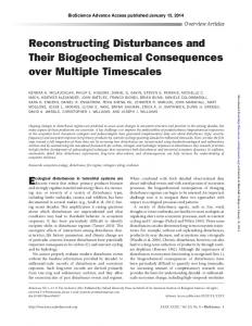
Figure 6: Two-dimensional Euclidean representations for discrimination probabilities (nonmetric MDS, Panel A) and for Fechnerian distances (metric MDS, Panel B) in Table 3. The MDS program used is PROXSCAL 1.0 in SPSS 11.5, minimizing raw stress. Sequence of 1’s and 2’s preceding a dash is the Morse code for the symbol following the dash. Insets are scree plots (normalized raw stress versus number of dimensions).

MDS can be used in conjunction with FSDOS, as a follow-up analysis once Fechnerian distances have been computed. A nonmetric version of MDS can be applied to Fechnerian distances (as opposed to discrimination probabilities directly) simply to provide a rough graphical representation for matrices like in Tables 3 and 4. More interestingly, a metric version of MDS can be applied to Fechnerian distances to test the hypothesis that Fechnerian distances, not restricted 5

We are grateful to Associate Editor for pointing this out to us.


29

0.10

0.10

0.06

0.06

0.02

0.02 1

2

3

1

4

2

S3L1L

L3L3L

S3L1S

L3L3S

4

S3L3L

L3L3L S3L3L

3

L3L3S S3L3S

L3L1L L3L1S L3L1L

Dimension 2

S3L3S

L3S3L

L3S3L L3S3S

L3L1S

A

Dimension 1

B

S3L1L S3L1S

L3S3S

Dimension 1

Figure 7: Same as Fig. 6, but for discrimination probabilities (nonmetric MDS, Panel A) and for Fechnerian distances (metric MDS, Panel B) in Table 4. L stands for long tone, S for short tone, while digits 1 an 3 show the lengths of the two pauses.

a priori to any particular class (except for being intrinsic), can be approximated by Euclidean distances (more generally, power-function Minkowski ones); the degree of approximation for any given dimensionality is measured by the achieved stress value. Geometrically, metric MDS on Fechnerian distances is an attempt to isometrically embed (i.e., map without distorting pairwise distances) the discrete object space in a low-dimensional Euclidean (or Minkowskian) space. Figures 6 and 7 provide a comparison of the metric MDS on Fechnerian distances with nonmetric MDS performed on discrimination probabilities directly, for the 10

10 submatrices presented in

Tables 3 and 4. Using the value of normalized raw stress as our criterion, the two-dimensional solution is almost equally good in both analyses. Therefore to the extent we consider the traditional MDS solution acceptable, we can view the Fechnerian distances in these two cases as being approximately Euclidean. The con…gurations of points obtained by metric MDS on Fechnerian

30


distances and nonmetric MDS on discrimination probabilities are more similar in Fig. 6 than in Fig. 7, indicating that MDS-distances provide a better approximation to Fechnerian distances in the former case. This may re‡ect the fact that the Kendall correlation between the probabilities and Fechnerian distances for Rothkopf’s data is higher than for Wish’s data (0.76 vs 0.68). A detailed comparison of the con…gurations provided by the two analyses, as well as such related issues as interpretation of axes are, however, beyond the scope of this paper.

6. General form of Regular Minimality. In continuous stimulus spaces it often happens that for a …xed value of x;

(x; y) achieves its minimum not at y = x but at some other value

of y; and for a …xed value of y;

(x; y) achieves its minimum at some value other than x = y.

It has been noticed since Fechner (1860), for example, that when x and x are presented in a succession, the second stimulus often seems larger (bigger, brighter, etc.) than the …rst: this is the classical phenomenon of “time error.” It follows that in a successive pair (x; y) the two elements maximally resemble each other when y is physically smaller than x: Borrowing the terminology from the theory of greater-less comparisons, Dzhafarov (2002d, 2003a) proposed to call the value of arg miny

(x; y) (i.e., the value of y at which

(x; y) achieves its minimum, for a …xed x) the

point of subjective equality, PSE, for x; and analogously, the value of arg minx

(x; y) is called the

PSE for y: Using this terminology, the general formulation of the Regular Minimality principle is as follows: (a) every x in the …rst observation area has a unique PSE in the second observation area; (b) every y in the second observation area has a unique PSE in the …rst observations area; and (c) y is the PSE for x if and only if x is the PSE for y: For a detailed discussion, see Dzhafarov (2002d, 2003a) and Dzhafarov and Colonius (2005a).


31

Table 5: A matrix of discrimination probabilities satisfying Regular Minimality in a non-canonical form. A canonical transformation of this matrix yields matrix M 1 of Table 1. M0 a b c d

a 0:6 0:9 1 0.5

b 0:6 0:9 0.5 0:7

c 0.1 0:8 1 1

d 0:8 0.1 0:6 1

Clearly, the formulation of Regular Minimality that we used so far, (3), is a special case: arg miny

(x; y) = x and arg minx

(x; y) = y (i.e., two physically identical stimuli are mutual

PSEs). As we know, this form of Regular Minimality is called canonical. It is possible that in discrete stimulus spaces Regular Minimality always has this special form, but it need not be so a priori. It seems useful therefore to reformulate the algorithm and interpretation of FSDOS under the assumption that Regular Minimality holds in its general form. Consider the following modi…cation of our toy example. Let the object space now be fa; b; c; dg and the initial matrix look as in Table 5. It is easy to see that Regular Minimality holds here, although not in a canonical form: every row contains a single minimal cell, and this cell is also minimal in its column. We can make a list of mutual PSEs and relabel them, assigning one and the same label to every pair of PSEs: (a; c) ! A; (b; d) ! B; (c; b) ! C; (d; a) ! D: With this relabeling, the matrix M 0 of Table 5 transforms into the matrix M 1 of our initial toy example (Table 1), with Regular Minimality now holding in the canonical form, (3). Due to Regular Minimality this can always be achieved by an appropriate relabeling. Having performed the Fechnerian analysis on M 1 and having computed the matrices L1 and G1 of Table2, we can return to the original labeling and present the Fechnerian distances and geodesic loops separately for the …rst and the second observation areas. A; B; C; D in L1 and G1 should be replaced with, respectively, a; b; c; d for the …rst observation area, and with

32


c; d; b; a for the second observation area. Denoting the overall Fechnerian distance G in the …rst and second observation areas by G(1) and G(2) ; respectively (not to be confused with the oriented Fechnerian distances distances G1 and G2 ), we will see, for instance, that G(1) (a; b) is 1.3, while G(2) (a; b) is 0.7, re‡ecting the fact that a; b are perceived di¤erently in the two observation areas. On the other hand, G(2) (c; d) is 1.3., the same as G(1) (a; b). This re‡ects the fact that c; d in the second observation area are PSEs for, respectively, a; b in the …rst observation area.

4. 1.

Concluding Remarks

Statistical issues. In some applications the frequency estimates of pij =

(si ; sj ) are

computed from samples su¢ ciently large to ignore statistical issues and treat FSDOS as being performed on essentially a population level. To a large extent this is how the theory of FSDOS is presented in this paper. The questions of …nding the joint sampling distribution for Fechnerian ^ ij (i; j = 1; 2; :::; N ) or joint con…dence intervals for Gij are beyond the scope of this distances G paper. We can, however, outline a general approach. The estimators Pîj of the probabilities pij are obtained as Rij 1 X ^ Xijk ; Pij = Rij k=1

where

Xij1 ; :::; XijRij

are random variables representing binary responses (1 = dif f erent,

0 = same). The index k may represent chronological trial numbers for (si ; sj ) ; di¤erent examples of this pair, di¤erent respondents, etc. Random variables Xijk and Xi0 j 0 k0 can be treated as stochastically independent, provided (i; j; k) 6= (i0 ; j 0 ; k 0 ). Assuming that Pr [Xijk = 1] does not vary too much as a function of k (i.e., ignoring such factors as fatigue, learning, and individual di¤erences), Pîj may be viewed as independent normally distributed variables with means pij and

Reconstructing Distances from Discriminability variances pij (1

33

pij ) =Rij ; from which it would follow that the joint distribution of the psychome-

tric lengths of all chains with distinct elements is asymptotically multivariate normal, with both the means and covariances being known functions of true probabilities pij . The problem then is reduced to …nding the (asymptotic) joint sampling distribution of the minima of psychometric lengths with common terminal points. Realistically, the problem is more likely to be dealt with by means of Monte Carlo simulations. Monte Carlo is also likely to be used for constructing joint con…dence intervals for Gij ; given a matrix of pîj : The procedure consists of repeatedly replacing the latter with matrices of pij that are subject to Regular Minimality and deviate from pîj less than some critical value (e.g., by the conventional chi-square criterion), and computing Fechnerian distances from each of these matrices.

2. Choice of object set. In some cases, as with Rothkopf’s (1957) Morse codes, the set S of objects used in an experiment or computation may contain all objects of a given kind. If such a set is too large or in…nite, however, one can only use a subset S 0 of the entire S: This gives rise to a problem: the Fechnerian distance G (a; b) between objects a; b 2 S 0 will generally depend on what other objects are included in S 0 : In a psychophysical experiment, when pairs of objects are presented repeatedly to a single observer, adding a new object s to S 0 may change the pairwise discrimination probabilities

(a; b) within the old subset. In a group experiment with each pair

presented just once, or for the “paper-and-pencil” perceivers, adding s to S 0 may not change discrimination probabilities; but this will still add new loops containing any given a; b 2 S 0 ; as a ()

result, the minimum psychometric length Lmin (si ; sj ) will generally decrease.6 6

This decrease must not be interpreted as a decrease in subjective dissimilarity. As mentioned earlier, Fechnerian distances are determined up to multiplication by an arbitrary positive constant, which means that only relative

34

Dzhafarov and Colonius A formal approach to this issue is to simply state that the Fechnerian distance between two

given objects is a relative concept: G (a; b) shows how far apart the two objects are “from the point of view”of a given perceiver and with respect to a given object set. This approach may be su¢ cient in a variety of applications, especially in psychophysical experiments with repeated presentations of pairs to a single observer: one might hypothesize that the observer in such a situation gets adapted to the immediate context of the objects in play, e¤ectively con…ning to it the subjective “universe of possibilities.”A discussion of this “adaptation to subspace”hypothesis can be found in Dzhafarov and Colonius (2005a). Like in many other situations involving sampling, however (including, e.g., sampling of respondents in a group experiment), one may only be interested in a particular subset S 0 of objects to the extent it is representative of the entire set S of objects of a particular kind. In this case one faces two distinctly di¤erent questions. The …rst question is empirical: is S 0 large enough (well chosen enough) for its further enlargements not to lead to noticeable changes in discrimination probabilities within S 0 ? This question is not FSDOSspeci…c, any other analysis of discrimination probabilities (e.g., MDS) will have to address it too. The second question is computational, and it is FSDOS-speci…c: provided the …rst question is answered in the a¢ rmative, is S 0 large (well chosen) enough for its further enlargements not to lead to noticeable changes in Fechnerian distances within S 0 ? A detailed discussion being outside the scope of this paper, we can only mention what seems to be an obvious approach: the a¢ rmative answer to second question can be given if one can show, by means of an appropriate version of subsampling, that the exclusion of a few objects from S 0 does not lead to changes in Fechnerian distances within the remaining subset.

Fechnerian distances G (a; b) =G (c; d) are meaningfully interpretable.


35

3. Other empirical procedures. The procedure of pairwise presentations with same-di¤erent judgments is the focal empirical paradigm for FSDOS. With some caution, however, FSDOS can also be applied to other empirical paradigms, such as that of identi…cation, mentioned in Section 1.3: all objects fs1 ; s2 ; :::; sN g are associated with rigidly …xed, normative reactions fR1 ; R2 ; :::; RN g (e.g., …xed names), and the objects are presented one at a time. Such an experiment results in the stimulus-response confusion probabilities

(si ; sj ) with which reaction Rj

(normatively reserved for sj ) is given to object si . FSDOS here can be applied under the additional assumption that

(si ; sj ) can be interpreted as 1

(si ; sj ). Regular Minimality here

means that each object si has a single modal reaction Rj (in the canonical form, Ri ), and then any other object causes Rj less frequently than si does. Thus understood, Regular Minimality is satis…ed, for example, in the data reported in Shepard (1957, 1958). We reproduce here one of the matrices from this work (Table6, rows are stimuli, columns normative responses, entries conditional probabilities

(si ; sj )), together with the matrix of Fechnerian distances. Geodesic

loops are not shown because the space fA; B; :::; Ig here turns out to be a “Fechnerian simplex”: a geodesic chain from a to b in this space is always the one-link chain (a; b). In a variant of the identi…cation procedure, the reactions may be preference ranks for objects fs1 ; s2 ; :::; sN g, R1 designating, say, the most preferred object, RN the least preferred. Suppose that Regular Minimality holds in the following sense: each object has a modal (most frequent) rank, each rank has a modal object, and Rj is the modal rank for si if and only if si is the modal object for Rj . Then the frequency

(si ; Rj ) can be taken as an estimate of 1

(si ; sj ), and the

data be subjected to FSDOS. The fact that these and similar procedures are used in a variety of areas (psychophysics, neurophysiology, consumer research, educational testing, political science), combined with the great simplicity of the algorithm for FSDOS, makes one hope that its potential

36


Table 6: M 2: one of the identi…cation probability matrices reported in Shepard (1957, 1958). G2: Fechnerian distances computed from matrix M 2: M2 A B C D E F G H I

A .678 0.167 0.06 0.015 0.037 0.027 0.011 0.016 0.005

B .148 0.544 0.07 0.104 0.068 0.029 0.033 0.027 0.016

C .054 0.066 0.615 0.016 0.12 0.053 0.015 0.031 0.011

D .03 0.077 0.015 0.542 0.057 0.015 0.145 0.046 0.068

E .025 0.053 0.107 0.057 0.46 0.036 0.049 0.069 0.02

F .02 0.015 0.067 0.005 0.075 0.715 0.016 0.096 0.021

G .016 0.045 0.022 0.163 0.057 0.015 0.533 0.053 0.061

H .011 0.018 0.03 0.032 0.099 0.095 0.052 0.628 0.018

I .016 0.015 0.014 0.065 0.03 0.014 0.145 0.034 0.78

G2 A B C D E F G H I

A 0 0.907 1.179 1.175 1.076 1.346 1.184 1.279 1.437

B 0.907 0 1.023 0.905 0.883 1.215 0.999 1.127 1.293

C 1.179 1.023 0 1.126 0.848 1.21 1.111 1.182 1.37

D 1.175 0.905 1.126 0 0.888 1.237 0.767 1.092 1.189

E 1.076 0.883 0.848 0.888 0 1.064 0.887 0.92 1.19

F 1.346 1.215 1.21 1.237 1.064 0 1.217 1.152 1.46

G 1.184 0.999 1.111 0.767 0.887 1.217 0 1.056 1.107

H 1.279 1.127 1.182 1.092 0.92 1.152 1.056 0 1.356

I 1.437 1.293 1.37 1.189 1.19 1.46 1.107 1.356 0

application sphere may be very large.

References Borg, I., & Groenen, P. (1997). Modern multidimensional scaling. New York: Springer-Verlag.

DeSarbo, W. S., Johnson, M. D., Manrai, A. K., Manrai, L. A., & Edwards, E. A. (1992) TSCALE: A new multidimensional scaling procedure based on Tversky’s contrast model. Psychometrika, 57, 43-70.

Dzhafarov, E. N. (2002a). Multidimensional Fechnerian scaling: Regular variation version. Journal of Mathematical Psychology, 46, 226-244.


37

Dzhafarov, E.N. (2002b). Multidimensional Fechnerian scaling: Probability-distance hypothesis. Journal of Mathematical Psychology, 46, 352-374.

Dzhafarov, E.N. (2002c). Multidimensional Fechnerian scaling: Perceptual separability. Journal of Mathematical Psychology, 46, 564-582.

Dzhafarov, E.N. (2002d). Multidimensional Fechnerian scaling: Pairwise comparisons, regular minimality, and nonconstant self-similarity. Journal of Mathematical Psychology, 46, 583-608.

Dzhafarov, E.N. (2003a). Thurstonian-type representations for “same-di¤erent”discriminations: Deterministic decisions and independent images. Journal of Mathematical Psychology, 47, 208228.

Dzhafarov, E.N. (2003b). Thurstonian-type representations for “same-di¤erent”discriminations: Probabilistic decisions and interdependent images. Journal of Mathematical Psychology, 47, 229243.

Dzhafarov, E.N., & Colonius, H. (1999). Fechnerian metrics in unidimensional and multidimensional stimulus spaces. Psychonomic Bulletin and Review, 6, 239-268.

Dzhafarov, E.N., & Colonius, H. (2001). Multidimensional Fechnerian scaling: Basics. Journal of Mathematical Psychology, 45, 670-719.

Dzhafarov, E.N., & Colonius, H. (2005a). Psychophysics without physics: A purely psychological theory of Fechnerian Scaling in continuous stimulus spaces. Journal of Mathematical Psychology, 49, 1-50.

38


Dzhafarov, E.N., & Colonius, H. (2005b). Psychophysics without physics: Extension of Fechnerian Scaling from continuous to discrete and discrete-continuous stimulus spaces. Journal of Mathematical Psychology, 49, 125-141.

Fechner, G. T. (1860). Elemente der Psychophysik [Elements of psychophysics]. Leipzig: Breitkopf & Härtel.

Indow, T. (1998). Parallel shift of judgment-characteristic curves according to the context in cutaneous and color discrimination. In C.E. Dowling, F.S. Roberts, P. Theuns (Eds.), Recent Progress in Mathematical Psychology (pp. 47-63). Mahwah, NJ: Erlbaum.

Indow, T., Robertson, A.R., von Grunau, M., & Fielder, G.H. (1992). Discrimination ellipsoids of aperture and simulated surface colors by matching and paired comparison. Color Research and Applications, 17, 6-23.

Izmailov, Ch. A., Dzhafarov, E. N, & Zimachev, M.M. (2001). Luminance discrimination probabilities derived from the frog electroretinogram. In: E. Sommerfeld, R. Kompass, T. Lachmann (Eds.) Fechner Day 2001 (pp. 206-211). Lengerich: Pabst Science Publishers.

Krumhansl, C.L. (1978). Concerning the applicability of geometric models to similarity data: The interrelationship between similarity and spatial density. Psychological Review, 85, 445-463.

Kruskal, J. B., & Wish, M. (1978). Multidimensional scaling. Beverly Hills: Sage.

Rothkopf, E. Z. (1957). A measure of stimulus similarity and errors in some paired-associate learning tasks. Journal of Experimental Psychology, 53, 94-102.

Reconstructing Distances from Discriminability Roweis, S. T. , &

39

Saul, L. K. (2000). Nonlinear dimensionality reduction by locally linear

embedding. Science, 290, 2323-2326. Sanko¤, D. & Kruskal, J. (1999). Time warps, string edits, and macromolecules. Stanford, CA: CSLI Publications. Shepard, R. N. (1957). Stimulus and response generalization: A stochastic model relating generalization to distance in psychological space. Psychometrika, 22, 325-345. Shepard, R. N. (1958). Stimulus and response generalization: Tests of a model relating generalization to distance in psychological space. Journal of Experimental Psychology, 55, 509-523. Shepard, R. N., and Carroll, J. D. (1966). Parametric representation of nonlinear data structures. In P. R. Krishnaiah (Ed.), Multivariate Analysis (pp. 561-592). New York: Academic Press. Tenenbaum, J. B., de Silva, V., & Langford, J. C. (2000). A global geometric framework for nonlinear dimensionality reduction. Science, 290, 2319-2323. Thurstone, L.L. (1927). A law of comparative judgments. Psychological Review, 34, 273-286. Tversky, A. (1977). Features of similarity. Psychological Review, 84, 327-352. Weeks, D. G., & Bentler, P. M. (1982). Restricted multidimensional scaling models for asymmetric proximities. Psychometrika, 47, 201-208. Wish, M. (1967). A model for the perception of Morse code-like signals. Human Factors, 9, 529-540. Zimmer, K., & Colonius, H. (2000). Testing a new theory of Fechnerian scaling: The case of auditory intensity discrimination. Journal of the Acoustical Society of America, 108, 2596.