Nov 8, 1999 - Local potentials that arise between the tip of an atomic force microscope (AFM) and a sample add to the free. AFM cantilever potential .... In practice, however, eq 5 does not hold because of systematic .... test case for the method. Such a ..... (35) Israelachvili, J. N. Intermolecular and Surface Forces, 2nd ed.;.
622
J. Phys. Chem. B 2000, 104, 622-626
Reconstructing Local Interaction Potentials from Perturbations to the Thermally Driven Motion of an Atomic Force Microscope Cantilever William F. Heinz,† Matthew D. Antonik,† and Jan H. Hoh*,†,‡ Department of Physiology, Johns Hopkins UniVersity School of Medicine, Baltimore, Maryland 21205, and Department of Chemical Engineering, Johns Hopkins UniVersity, Baltimore, Maryland 21218 ReceiVed: September 22, 1999; In Final Form: NoVember 8, 1999
Local potentials that arise between the tip of an atomic force microscope (AFM) and a sample add to the free AFM cantilever potential and thereby affect the thermally driven motion of the cantilever. Here we present a general framework for isolating the tip-sample interaction potential from the total potential based on the analysis of the perturbations to the thermally driven motion of the cantilever. To establish appropriate experimental parameters, we first examine the behavior of the free cantilever in air and in water. We then measure the total and interaction potentials of an AFM cantilever in a low salt aqueous solution, a classical electrical double-layer interaction, and validate the approach by reconstructing the force curve (force law) from the force gradients derived from the potentials. We also present three-dimensional representations of the total cantilever potential and the tip-sample interaction potentials as a function of tip-sample separation.
Introduction The atomic force microscope (AFM)1 is emerging as an important tool for measuring the spatial distribution of forces between nanometer scale objects. In the most widely used approach for this type of measurement, the AFM cantilever is used as a simple Hookian spring, and dc (time-averaged or “static”) deflections of the cantilever are measured as a function of the separation distance between the tip (or some molecule attached to it) and the sample. These force curves are interpreted using a wide range of force laws, depending on the type of interaction that is being studied.2 More recently, the ac (dynamic) motions of thermally or externally driven AFM cantilevers have been used to probe interactions.3-10 Perturbations to the thermally driven motion of particles have been used in a number of systems to study interactions between particles.11-13 In addition, the thermal motions of force probes have been used to measure the spring constants of optical traps,14,15 glass fibers,16 and AFM cantilevers.17-21 The basis for these types of measurements is that for ideal particles in Brownian motion under the influence of an unknown potential, the distribution of particle positions and the deviations of trajectories from the ideal case can give information about the potential. For the case of AFM cantilevers this idea is supported by a number of theoretical studies that describe the thermally driven motion of cantilevers in air and vacuum,17-25 as well as in fluid.26-28 However, this approach has been used only in a limited number of cases. Changes in the thermally driven oscillations of AFM cantilevers have been used to study the collapse of a polymer brush,4-6 the potentials due to the ordering of water near a calcite surface,7 and the electrostatic doublelayer force.8 In the last two studies, potential wells were calculated from the distribution of cantilever deflections. These wells describe the total tip potential, which includes any interaction potentials as well as the spring potential of the * To whom correspondence should be addressed. † Department of Physiology. ‡ Department of Chemical Engineering.
cantilever. Here, we present a general formulation for calculating potential wells solely from the thermally induced deflections of a cantilever. We apply this analysis to an electrostatic double layer potential, isolate the tip-sample interaction potential by removing the cantilever potential from the total potential, and present 3-D representations of the potential surfaces by plotting them as functions of tip-sample separation distance. Theory and Experimental Approach To assess the effects an external potential will have on the motion of a cantilever, we first consider the general case of superimposed potentials. We treat the deflections, x, of a spring about its time-averaged equilibrium deflection as a Boltzmann distribution, where the probability, p(x), that the cantilever is at a given deflection, x, depends on the potential V(x) that can be a function of tip-sample separation distance, d. Note that V(x) is the total potential and depends on the cantilever potential and any external potential such as one that may form between the tip and sample. Thus, the probability distribution of the cantilever is given by
p(x) ) p0e-V(x)/kBT
(1)
where p0 is a normalization factor. Taking the log of both sides and rearranging, we can express V(x) as
V(x) ) -kBT ln(p(x)/p0)
(2)
We assume that there are only two contributions to the total potential, the cantilever potential,VC(x), and the tip-sample interaction potential, VI(x), and therefore
V(x) ) VC(x) + VI(x)
(3)
The tip-sample interaction potential can then be isolated by subtracting the cantilever potential from the total potential:
10.1021/jp993394t CCC: $19.00 © 2000 American Chemical Society Published on Web 12/22/1999
Local Interaction Potentials of an AFM Cantilever
VI(x) ) -kBT
{
[ ]}
VC(x) p(x) + ln kBT p0
J. Phys. Chem. B, Vol. 104, No. 3, 2000 623
(4)
In an AFM force measurement the interaction potential depends on the tip-sample separation distance, d. Thus, the above equations can also be expressed using the distance dependent terms V(x,d), VI(x,d), and p(x,d). In the ideal case the cantilever alone is modeled as a simple harmonic oscillator (SHO), and when VI(x) ) 0
VC(x) )
[ ]
p(x) kx2 ) -kBT ln 2 p0
(5)
In practice, however, eq 5 does not hold because of systematic errors inherent in the experimental conditions and instrument limitations. To begin with, Butt20 has shown that the first 10 vibration modes of an AFM cantilever make up 96% of the root-mean-squared (RMS) deflection amplitude in air. With the data acquisition system described here, which, at 1 MHz, is severalfold faster than most commercial AFMs, only the contributions of the first few modes (n e 5) of the most flexible cantilevers (∼0.01 N/m) can be measured. Even if the data acquisition rates were sufficiently high, the deflections in higher modes are not accurately measured because of limitations in the conventional beam deflection detection system.29-32 In solution the situation is further complicated by dissipative effects that strongly affect the shapes of the higher modes. The shape of the fundamental mode, however, is virtually unaffected and, in the neighborhood around the resonance peak, can be modeled as an SHO.26 Another complicating factor is electronic noise. These limitations to accurately reconstructing the true cantilever potential also affect the determination of VI. To account for these systematic errors, we introduce an error factor, �, into the right side of eq 3:
V(x) ) �(VC(x) + VI(x))
(6)
The experimental approach to measuring interaction potentials using eq 6 is to first measure the thermally driven motion of the AFM cantilever at some distance where there is no tipsample interaction. These deflection measurements are then used to produce a probability distribution for the cantilever, from which an apparent cantilever potential well can be reconstructed. The error factor, �, is determined from the ratio of the true cantilever spring constant determined in air21 to the apparent cantilever spring constant (� ) k/kapparent). The tip is then brought toward the sample so that the tip is within range of the interaction potential, and the thermally driven motion of the cantilever is again recorded. The apparent cantilever potential is subtracted from this total potential as in eq 4 to give the tipsample interaction potential. After scaling by �, this potential is used to calculate the force gradient at that distance. If the tip is initially far from the sample surface and the tip-sample distance is varied slowly during the measurement, the tipsample interaction force as a function of distance can be constructed from integration of the force gradient calculated from the thermal motions of the cantilever. Materials and Methods Instrumentation. A Nanoscope IIIa controller and a multimode atomic force microscope (Digital Instruments Inc., Santa Barbara, CA) equipped with a phase extender and either a J-type or D-type scanner was used for all experiments presented. The cantilever deflections were measured using the standard optical
lever system customized with a low-noise infrared laser. Deflection voltages from the photodiode were collected using a commercial Signal Access Module (Digital Instruments) connected in-line between the microscope base and the extender module, and a 12 bit 1 MHz A/D board (NB-A2000; National Instruments, Austin, TX) installed on a Macintosh computer. This deflection signal is essentially unfiltered by the Nanoscope through the entire data acquisition range (J. Cleveland, personal communication). The raw deflection signal was amplified using a home-built amplifier (300 kHz maximum bandwidth at 10x amplification). Data collection was performed using custom software written in LabVIEW (National Instruments). It is important to note that calibration of the optical-lever sensitivity prior to force measurements is essential to accurately convert the photodiode output voltage to cantilever deflection.33 Sample Preparation and Data Collection. Mica disks (12 mm, grade V1; Asheville-Schoonmaker Mica Co., Newport News, VA) were glued to stainless steel stubs and cleaved to expose a fresh surface immediately before use. V-shaped silicon nitride cantilevers were either 140 or 320 µm from the base to the free end with 22 µm wide legs and had nominal force constants of 0.1 and 0.01 N/m, respectively (Park Scientific Instruments, Sunnyvale, CA). Force curves were collected using the Nanoscope control software to drive the z-piezo motion (maximum speed 20 µm/s) and the data acquisition system described above to record cantilever deflections. Typically, data were collected at rates of 0.5-1 MHz. These data were later band-pass-filtered between 130 Hz and 100 kHz. Data Analysis. Data were analyzed using a custom software tool written in the Interactive Data Language (Research Systems, Inc., Boulder, CO) programming environment, called “MegaHertz Force Curves” (MFC). MFC reads, displays, filters, and analyses MHz force curves using the approach outlined above. Results Free Cantilever Potential. To determine V0(x) we first examine the behavior of the free cantilever in air and water. In air a typical 140 µm cantilever has a resonant frequency of 28.5 kHz and the thermally driven motion has a RMS amplitude of 0.51 nm (Figure 1a). To achieve a Boltzmann-like sampling, the thermally driven deflections used to construct p(x) need to be uncorrelated. The correlation time of a simple harmonic oscillator is on the order of Q/f0, where Q is the quality factor of the oscillator and f0 is the resonant frequency. The extent of correlation can also be measured by the autocorrrelation function. For the 140 µm cantilever in air this function approaches zero within several milliseconds (Figure 1b). Uncorrelated deflection data for p(x) can be achieved in two ways. The first is to sample the deflection using a sampling period longer than the correlation time. The second is to collect a large number of deflections sampled with a period shorter than the correlation time. In the first case, individual deflections are uncorrelated from each other. In the second case they are correlated with their neighbors but uncorrelated from the vast majority of deflections in the data set. Both approaches give the same values for RMS deflections and apparent cantilever potentials (data not shown). Thus, by collecting data at a high sampling rate for more than several milliseconds a Boltzmannlike sampling is produced. This results in a Gaussian distribution of cantilever deflections of the free cantilever (Figure 1c). The natural logarithm of this distribution gives the apparent cantilever potential (V0(x)), which can be fit to a quadratic (Figure 1d). Similar results are obtained in water, with the exception that the resonant frequency of the cantilever is reduced
624 J. Phys. Chem. B, Vol. 104, No. 3, 2000
Figure 1. Thermally driven motion of an AFM cantilever in air and water. (a) Deflections of a 140 µm V-shaped cantilever measured as a function of time. To improve clarity, only one out of every 500 points is plotted. (b) Autocorrelation function of the data. The signal becomes uncorrelated within several milliseconds. (c) Probability distribution of the cantilever deflection. The distribution is Gaussian. (d) Apparent cantilever potential. This is obtained by taking the natural logarithm of the probability distribution and multiplying by kBT. This potential can be fit to a quadratic. (e-h) Same as (a-d) for the same cantilever in water.
and the typical correlation time is much shorter than that in air (Figure 1e-h). The reduction in resonant frequency results from an increase in the effective mass of the cantilever, due to the presence of the liquid.34 The error factor, �, is determined from the ratio of the spring constant determined by fitting the resonance peak in air to that determined from the fit to the well. In this case, � was near unity. Electrostatic Potentials. To demonstrate that the interaction potential can be calculated from just the thermal motions of the cantilever, we collected force curves of a bare silicon-nitride tip interacting with a mica surface in an aqueous environment. Both the tip and the mica are negatively charged, and at separation distances greater than a few nanometers the interaction is dominated by electrostatic repulsion. This electrostatic double-layer force is well modeled by the Derjaguin, Landau, Verwey, and Overbeek theory (DLVO),35 has been studied by many groups using the AFM,36-42 and therefore provides a good test case for the method. Such a repulsive interaction is readily captured in an AFM force curve (Figure 2a). Because the decay length of this curve is 6.8 nm, which agrees with the Debye
Heinz et al.
Figure 2. Perturbations to the thermally driven motion of an AFM cantilever by an electrostatic potential. (a) AFM force curve of a silicon nitride tip on a mica substrate in 2 mM KCl. The approach speed was 20 nm/s. (b) Thermal noise contribution to the force curve. The curve in (a) was band-pass filtered (130 Hz to 100 kHz). (c) Total potentials at three different z-piezo positions distances (marked O, 4, and 0 in (a)). (d) Tip-sample interaction potentials as a function of cantilever deflection and z-piezo position.
length of 6.9 nm for the 2 mM KCl solution we used, we conclude that the repulsion is due to the electrostatic doublelayer force. To examine the effect of the electrostatic potential on the thermally driven motion of the AFM cantilever, we first take this force curve and remove low-frequency contributions (Figure 2b). In effect, we remove the dc component of the force curve. We typically use a 130 Hz filter, although in our experience the final result is not particularly sensitive to the low-frequency cutoff. In the case described here, we find no differences between 50 and 500 Hz. Taking the natural logarithm of the probability distribution of this signal gives the total potential, V(x,d) (Figure 2c). The total potential contains the apparent cantilever potential and the electrostatic interaction potential, which varies with the z-piezo position and, therefore, the tip-sample separation distance. The piezo position and the separation distance are related by a simple transformation.43 At relatively large separation distances, there are no measurable tip-sample interactions (position marked by O in Figure 2a). This allows the potential
Local Interaction Potentials of an AFM Cantilever
J. Phys. Chem. B, Vol. 104, No. 3, 2000 625
Figure 4. dc force curve reconstruction from thermal noise: (a) force gradient calculated from smoothed raw data (O) and interaction force gradient calculated from the thermal noise and scaled (s); (b) dc force curve from smoothed raw data (O) and interaction force curve calculated from thermal noise and scaled (s). The dashed vertical lines mark the jump-to-contact point.
Figure 3. 3D potential wells calculated from thermal noise for an AFM cantilever in an electrostatic double layer potential: total well (a-d) and interaction potential well (e-h). The wells are ∼10kBT deep and ∼6 nm wide. The labeled z-axis of the surface corresponds to the z-piezo position (95 nm) as in Figure 2. In all panels the axis labels are positioned at the cantilever potential with zero contribution from the interaction. Key: (a) and (e) perspective view; (b) and (f) head-on view; (c) and (g) side view; (d) and (h) top view.
for the free cantilever, V0(x), to be determined. By subtracting this potential from the total potential (Figure 2c) a tip-sample interaction potential at any separation distance (marked O, 0, and 4 in Figure 2a) can be isolated (Figure 2d). The total and interaction potentials calculated at all separation distances along the force curve can be represented as 3-dimensional surfaces (Figure 3). The fluctuations in the potential at large deflections are due to the low thermal sampling of those high-energy deflections. Because the cantilever spends relatively little time at large deflections, those regions contribute a small amount to the probability distribution, and the natural logarithm exaggerates the contribution of small probability values relative to larger ones. Reconstructing the Force Curve. The potential at any given separation distance is directly related to the force law by a derivative. For simple potentials, the force gradient is essentially constant over the small distances that the cantilever explores thermally, and the interaction potential at that separation distance appears parabolic. The second derivative of this potential gives the local force gradient and should equal the slope in the force curve at that separation distance. Because, in this case, the spring constant of the SHO is equivalent to the second derivative of
the potential, we fit the interaction potential data to a SHO potential to obtain the local force gradient (Figure 4a). In addition, assuming that the tip-sample interaction at large distances is zero, it should be possible to integrate the force gradient as a function of distance and reconstruct the dc component of the force curve (Figure 4b). For both the force gradient and the reconstructed dc force curve, the measured potentials are scaled by � (for this force curve � was 2.25). If they are not scaled, the force gradient and the reconstructed force curve calculated from the thermal noise do not agree with the directly measured values. Discussion Perturbations to the thermally driven motion of small particles can be used to study forces acting on them. The AFM is a sensitive force-measuring device that can be used to measure the thermally driven motion of a cantilever. Earlier work has shown that this motion is influenced by external potentials. Willemsen et al.8 and Cleveland et al.6 presented total potentials calculated from a Boltzmann-like sampling of cantilever deflections. Here we extend this approach to isolate the tip-sample interaction by subtracting the cantilever potential from the total potential. Further we demonstrate the validity of this method by reconstructing a known force law from the thermally driven motion of a cantilever. Reconstructing the force curve from the thermal noise assumes that the interaction force is linear (the force gradient is constant) over the range of thermally driven cantilever deflections. For weak cantilevers or for very steep or multiwelled potentials, however, the interaction potentials are not quadratic and hence do not yield a simple force gradient. Such a case was seen by Cleveland et al.6 in which hydration layers gave rise to multiple wells in the total potential. In such cases,
626 J. Phys. Chem. B, Vol. 104, No. 3, 2000 reconstructing the force law from the interaction potential well is more complicated. Of course, the shape of the interaction potential as well as how that potential changes with separation distance can still be useful. We further assume that the free cantilever noise does not change with separation distance. This is a reasonable assumption for small changes in separation distance but may not hold for large changes. For a driven oscillating cantilever in solution it is readily observed that the amplitude of the oscillation changes as the cantilever approaches a surface from a large distance. This change in amplitude occurs many micrometers from the surface and thus is not related to a tip-sample interaction but a hydrodynamic coupling of the cantilever to the sample.44 The laser used in the optical detection scheme can be a source of error. At a given tip-sample separation distance, fluctuations in the laser power can cause local heating/cooling of the cantilever, increasing or decreasing the size of the thermal motions of the beam.24,28 Pointing instability of the laser spot can also result in erroneous deflection measurements. The pointing instability is reduced in our case by using a low-noise infrared laser to detect cantilever deflections. Others have minimized these errors by delivering laser light to the AFM head with single-mode optical fibers.6 Because the power fluctuations and the pointing instability occur on a relatively long time scale, removing the low-frequency contributions to the cantilever deflections also reduces these errors. Last, our treatment of the error factor, �, requires that it remains constant at all positions along the force curve. Of course, � can be distance dependent, and if that dependence is known, then the interaction potential can be recovered. Here we treat limitations in bandwidth and the optical detection system and any other systematic errors as constant at all positions along the force curve. Conclusion We have presented a general approach to measuring local interaction potentials between an AFM tip and a sample surface based solely on the perturbations to the thermally driven motion of the cantilever. A local force gradient can be determined from the interaction potential, and the dc force curve can be calculated by integration of this force gradient. We also present 3-dimensional reconstructions of the total and interaction potentials. Unlike traditional dc force measurements, this technique allows the determination of the local force gradient without changing the z-piezo position. In principle, for some potentials the tipsample separation distance can be determined without collecting a complete force curve. This offers the possibility of a constantforce-gradient feedback mechanism. Furthermore, our approach provides a framework that can be extended to include more complex potentials than the one presented here. Acknowledgment. This work was supported in part by grants from the Council for Tobacco Research and the Whitaker Foundation for Biomedical Engineering. References and Notes (1) Binnig, G.; Quate, C. F.; Gerber, C. Phys. ReV. Lett. 1986, 56, 930. (2) Heinz, W. F.; Hoh, J. H. Trends Biotechnol. 1999, 17, 143. (3) Cleveland, J. P.; Anczykowski, B.; Schmid, A.; Elings, V. Appl. Phys. Lett. 1998, 72, 2613.
Heinz et al. (4) Roters, A.; Gelbert, M.; Schimmel, M.; Ruhe, J.; Johannsmann, D. Phys. ReV. E 1997, 56, 3256. (5) Roters, A.; Johannsmann, D. J. Phys. Condens. Matter 1998, 8, 7561. (6) Roters, A.; Schimmel, M.; Ruhe, J.; Johannsmann, D. Langmuir 1998, 14, 3999. (7) Cleveland, J. P.; Schaffer, T. E.; Hansma, P. K. Phys. ReV. B 1995, 52, 8692. (8) Willemsen, O. H.; Snel, M. M. E.; Kuipers, L.; Figdor, C. G.; Greve, J.; Grooth, B. G. D. Biophys. J. 1999, 76, 716. (9) Lantz, M.; Y. Z. Liu; Cui, X. D.; Tokumoto, H.; Lindsay, S. M. Surf. Interface Anal. 1999, 27, 354. (10) Han, W. H.; Lindsay, S. M. Appl. Phys. Lett. 1998, 72, 1656. (11) Radler, J.; Sackmann, E. Langmuir 1992, 8, 848. (12) Mason, T.; Ganesan, K.; vanZanten, J.; Wirtz, D.; Kuo, S. Phys. ReV. Lett. 1997, 79, 3282. (13) Mehta, A.; Finer, J.; Spudich, J. Proc. Natl. Acad. Sci. U.S.A. 1997, 94, 7927. (14) Florin, E.; Pralle, A.; Stelzer, E.; Horber, H. J. Appl. Phys. A Mater. Sci. Proc. 1998, 66, S75. (15) Veigel, C.; Bartoo, M. L.; White, D. C.; Sparrow, J. C.; Molloy, J. E. Biophys. J. 1998, 75, 1438. (16) Tokunaga, M.; Aoki, T.; Hiroshima, M.; Kitamura, K.; Yanagida, T. Biochem. Biophys. Res. Commun. 1997, 231, 566. (17) Hutter, J.; Bechoefer, J. ReV. Sci. Instrum. 1993, 64, 1868. (18) Hutter, J.; Bechoefer, J. ReV. Sci. Instrum. 1993, 64, 3342. (19) Cleveland, J. P.; Manne, S.; Bocek, D.; Hansma, P. K. ReV. Sci. Instrum. 1993, 64, 403. (20) Butt, H. J.; Jaschke, M. Nanotechnolgy 1995, 6, 1. (21) Walters, D. A.; Cleveland, J. P.; Thomson, N. H.; Hansma, P. K.; Wendman, M. A.; Gurley, G.; Elings, V. ReV. Sci. Instrum. 1996, 67, 3583. (22) Sader, J. E.; Larson, I.; Mulvaney, P.; White, L. R. ReV. Sci. Intsrum. 1995, 66, 3789. (23) Rabe, U.; Janser, K.; Arnold, W. ReV. Sci. Instrum. 1996, 67, 3281. (24) Li, B. Q.; Lin, J.; Wang, W. U. J. Micromech. Microeng. 1996, 6, 330. (25) Salapaka, M. V.; Bergh, H. S.; Lai, J.; Majumdar, A.; Mcfarland, E. J. Appl. Phys. 1997, 81, 2480. (26) Sader, J. E. A. J. Appl. Phys. 1998, 84, 64. (27) Gittes, F.; Schmidt, C. Eur. Biophys. J. Biophys. Lett. 1998, 27, 75. (28) Ratcliff, G. C.; D. A. Erie; Superfine, R. Appl. Phys. Lett. 1998, 72, 1911. (29) The calibration of the cantilever deflections is performed by ramping the sample into contact with the tip and pushing on the tip for a known distance in z. The slope of the resulting deflection vs piezo position curve in contact is adjusted to unity, setting the conversion factor from optical detector voltage to nanometers. This procedure assumes that only the fundamental bending mode of the cantilever contributes to the voltage shift during a measurement. In fact, because the optical lever detection system measures the end slope of the cantilever, not the actual deflection, higher bending modes can contribute to the end slope without changing the deflection of the cantilever (or vice versa), resulting in erroneous deflection values. Using direct methods to measure cantilever deflection or the shape of the cantilever avoids this problem.28,30 (30) Hlady, V.; Pierce, M.; Pungor, A. Langmuir 1996, 12, 5244. (31) Rabe, U.; Janser, K.; Arnold, W. ReV. Sci. Instrum. 1996, 67, 3281. (32) Sasaki, M.; Hane, K.; Okuma, S.; Bessho, Y. ReV. Sci. Instrum. 1994, 65, 1930. (33) D’Costa, N. P.; Hoh, J. H. ReV. Sci. Instrum. 1995, 66, 5096. (34) Butt, H. J.; Siedle, P.; Seifert, K.; Fendler, K.; Seeger, T.; Bamberg, E.; Weisenhorn, A. L.; Goldie, K.; Engel, A. J. Microsc. 1993, 169, 75. (35) Israelachvili, J. N. Intermolecular and Surface Forces, 2nd ed.; Academic Press: New York, 1992. (36) Ducker, W. A.; Senden, T. J.; Pashley, R. M. Nature. 1991, 353, 239. (37) Butt, H. J. Biophys. J. 1991, 60, 1438. (38) Biggs, S.; Proud, A. D. Langmuir 1997, 13, 7202. (39) Hillier, A. C.; Kim, S.; Bard, A. J. J. Phys. Chem. 1996, 100, 18808. (40) Larson, I.; Drummond, C. J.; Chan, D. Y. C.; Grieser, F. Langmuir 1997, 13, 2109. (41) Raiteri, R.; Gratarola, M.; Butt, H. J. J. Phys. Chem. 1996, 100, 16700. (42) Heinz, W. F.; Hoh, J. H. Biophys. J. 1999, 76, 528. (43) Butt, H. J. Biophys. J. 1992, 63, 578. (44) deSouza, E. F.; Douglas, R. A.; Teschke, O. Langmuir 1997, 13, 6012.