Jun 11, 2018 - E-mail: filippo[email protected] ...... to inferÏ and itsfluctuation properties, but also because in this way we could manage to measure the mean ...
Quantum Science and Technology
Related content
PAPER
Reconstructing quantum entropy production to probe irreversibility and correlations To cite this article: Stefano Gherardini et al 2018 Quantum Sci. Technol. 3 035013
View the article online for updates and enhancements.
- Measures and applications of quantum correlations Gerardo Adesso, Thomas R Bromley and Marco Cianciaruso - Time-reversal symmetric work distributions for closed quantum dynamics in the histories framework Harry J D Miller and Janet Anders - The role of quantum information in thermodynamics—a topical review John Goold, Marcus Huber, Arnau Riera et al.
This content was downloaded from IP address 150.217.251.67 on 19/06/2018 at 15:05
Quantum Sci. Technol. 3 (2018) 035013
https://doi.org/10.1088/2058-9565/aac7e1
PAPER
RECEIVED
2 October 2017
Reconstructing quantum entropy production to probe irreversibility and correlations
REVISED
21 May 2018 ACCEPTED FOR PUBLICATION
25 May 2018
Stefano Gherardini1,2,3, Matthias M Müller1, Andrea Trombettoni4,5,6, Stefano Ruffo5,6,7 and Filippo Caruso1,8
PUBLISHED
1
11 June 2018
2 3 4 5 6 7 8
Department of Physics, LENS and QSTAR, University of Florence, via G. Sansone 1, I-50019 Sesto Fiorentino, Italy Department of Information Engineering, University of Florence, via S. Marta 3, I-50139 Florence, Italy INFN, Sezione di Firenze, Sesto Fiorentino, Italy CNR-IOM DEMOCRITOS, via Bonomea 265, I-34136 Trieste, Italy SISSA, via Bonomea 265, I-34136 Trieste, Italy INFN, Sezione di Trieste, I-34151 Trieste, Italy ISC-CNR, Via Madonna del Piano 10, I-50019 Sesto Fiorentino, Italy Author to whom correspondence should be addressed.
E-mail: filippo.caruso@unifi.it Keywords: quantum thermodynamics, quantum entropy, quantum measurements, irreversibility, open quantum systems
Abstract One of the major goals of quantum thermodynamics is the characterization of irreversibility and its consequences in quantum processes. Here, we discuss how entropy production provides a quantification of the irreversibility in open quantum systems through the quantum fluctuation theorem. We start by introducing a two-time quantum measurement scheme, in which the dynamical evolution between the measurements is described by a completely positive, trace-preserving (CPTP) quantum map (forward process). By inverting the measurement scheme and applying the timereversed version of the quantum map, we can study how this backward process differs from the forward one. When the CPTP map is unital, we show that the stochastic quantum entropy production is a function only of the probabilities to get the initial measurement outcomes in correspondence of the forward and backward processes. For bipartite open quantum systems we also prove that the mean value of the stochastic quantum entropy production is sub-additive with respect to the bipartition (except for product states). Hence, we find a method to detect correlations between the subsystems. Our main result is the proposal of an efficient protocol to determine and reconstruct the characteristic functions of the stochastic entropy production for each subsystem. This procedure enables to reconstruct even others thermodynamical quantities, such as the work distribution of the composite system and the corresponding internal energy. Efficiency and possible extensions of the protocol are also discussed. Finally, we show how our findings might be experimentally tested by exploiting the state of-the-art trapped-ion platforms.
1. Introduction The advent of the thermodynamics laws and their following development, from the theoretical side, and the construction of heat engines, from the technological one, drove in the 18th and 19th centuries an astonishing series of important scientific discoveries and social transformations. The crucial point was the use of heat to produce work, which corresponds to take a disordered form of energy and convert (a part of) it into a mechanical one [1]. In the last decades, a breakthrough in non-equilibrium thermodynamics was given by the Jarzynski equality [2], which relates the free-energy between two equilibrium states to an exponential average of the work done on the system, over an ideally infinite number of repeated non-equilibrium experiments. This result links together free-energy differences to work measurements along an ensemble of trajectories in the phase space of the system with same energy contribution [3]. The Jarzynski equality can be derived also from the Crooks © 2018 IOP Publishing Ltd
Quantum Sci. Technol. 3 (2018) 035013
S Gherardini et al
fluctuation theorem [4], which formalizes the existence of symmetry relations for the probability distribution of thermodynamic quantities during the forward and reverse transformations that the system undergoes due to external actions. Generalized versions of the Jarzynski equality for non-equilibrium steady states from Langevin dynamics and non-equilibrium systems subjected to feedback control have been proved, then, respectively in [5, 6]. From the experimental side, the Jarzynski equality and its generalizations have been tested by a wide range of experiments, for example to determine the folding and unfolding free energies of a small RNA hairpin [7], or to prove the fundamental principle given by the information-to-heat engine, converting information into energy by means of feedback control [8]. Even from a purely classical point of view, the notion of thermodynamics quantities such as work, heat and entropy production have been extended to the level of individual trajectories of well-defined non-equilibrium ensembles by the stochastic thermodynamics [9, 10], which has allowed for the introduction of a generalized fluctuation-dissipation theorem involving entropy production. At the same time, the attention moved also towards the attempts to build a thermodynamic theory for quantum systems to exploit the power and the processes of quantum physics [11–14]. This field of research, known as quantum thermodynamics, aims at characterizing the thermodynamical aspects behind the quantum mechanical processes, defining the role of quantum coherence and measurements for such transformations [15–18]. Quantum thermodynamics, moreover, provides the theoretical tools to describe and build efficient quantum heat engines [19–21]. One of the major goals of quantum thermodynamics is the definition and characterization of irreversibility in quantum processes. This could have a significant impact on technological applications for the possibility of producing work with heat engines at high efficiency using systems where quantum fluctuations are important; in this regard, a detailed analysis about the aspects that define the work done by a quantum system can be found in [22]. The quantum work and its distribution are generally defined by taking into account also the role of quantum measurements and, consequently, the sensitivity of the system to the interactions with the measurement apparatus [23–26]. Recently a novel definition of quantum work has been proposed in [27], in which the work is a thermodynamic quantity depending only on the quantum system and not on the measurement apparatus. The importance of defining the concept of irreversibility in quantum thermodynamics can be hardly overestimated, as one can appreciate by considering its classical counterpart. As well-known, in classical mechanics the solutions of the dynamical equations of motion are unique and the motion along the trajectories in phase space can be inverted to retrieve all the states previously occupied by the system [28]. However, the time inversion in experiments with a macroscopic number of particles cannot be practically performed. As a consequence of the information loss and of the fact that is very improbable to occupy the same state at a later time, we have to resort to a statistical description of the system. In classical thermodynamics this is the origin of the irreversibility of the system dynamics. Similarly, in quantum mechanics the dynamics of the wave function and more generally of the density matrix can be reversed in time, and it ensues the corresponding need to characterize and quantify, where possible, irreversible quantum processes [29, 30]. The typical instance is given by the thermalization of an open system, where the dissipative processes taking place due to the interaction of the system with its environment degrade the quantum nature of the system and the coherence of the quantum states [31, 32]. Along this line, several studies have shown how to derive the quantum version of the fluctuationdissipation theorem, both for closed [33, 34] and open quantum systems [35–41]. Recently, in [42] a fully quantum fluctuation theorem have been formulated, explicitly including the reservoir exchanging energy with the system, and a control system driving its dynamics. In [43, 44], moreover, experimental tests of the quantum version of the Jarzynski identity [45–47] for work distributions are shown. Considerable efforts have been made in measuring irreversibility, and, consequently, the stochastic entropy production in quantum thermodynamics [48–51]. The ratio between the probability to observe a given quantum trajectory and its time-reversal is related to the amount of heat exchanged by the quantum system with the environment [52]. Such knowledge leads then to experimental procedures for the measure of the heat backflow with the environment, even if the latter in particular, is not necessarily correlated with the information backflow from the reservoir to the quantum system [53]. Lately, it has been experimentally proved that irreversibility in quantum non-equilibrium dynamics can be partially rectified by the presence of an intelligent observer, identified by the well-known Maxwellʼs demon [54, 55], which manages to assess additional microscopic informational degrees of freedom due to a proper feed-forward strategy [56]. Instead, regarding the reconstruction of the fluctuation properties of general thermodynamical quantities, in [57–60] an interferometric setting for the measurement of the characteristic function of the work distribution is introduced and proposed as the key element to properly design inference strategies [61]. This method, then, has been generalized for open quantum systems, as shown in [62, 63]. In [64], instead, a method for the sampling of the work distribution by means of a projective measurement at a single time is shown, motivating a novel quantum algorithm for the estimation of free energies in closed quantum systems. In the present work we address three issues. (i) We discuss how to relate the stochastic entropy production to the quantum fluctuation theorem, generalizing the Tasaki–Crooks theorem for open systems. This relation is 2
Quantum Sci. Technol. 3 (2018) 035013
S Gherardini et al
obtained via the evaluation of the irreversibility of the quantum dynamics. (ii) Then, once the stochastic quantum entropy production has been defined and characterized, we introduce a protocol to reconstruct it from the measurement data, possibly with the minimum amount of resources. Here, we propose a procedure to reconstruct the stochastic entropy production of an open quantum system by performing repeated two-time measurements, at the initial and final times of the system transformation. In particular, the proposed reconstruction algorithm requires to determine the characteristic function of the probability distribution of the stochastic quantum entropy production. Indeed, by means of a parametric version of the integral quantum fluctuation theorem, we can derive the statistical moments of the entropy production. Moreover, we also prove that with this procedure the number of required measurements scales linearly with the system size. (iii) By assuming that the quantum system is bipartite, we apply the reconstruction procedure both for the two subsystems and for the composite system by performing measurements, respectively, on local and global observables. The comparison between the local and the global quantity allows us to probe the presence of correlations between the partitions of the system. The manuscript is organized as follows. Section 2 reviews the quantum fluctuation theorem, introducing the definition of stochastic quantum entropy production. Section 3 analyzes the physical meaning of thermodynamic irreversibility by applying a two-time measurement scheme, and shows the relation between the mean entropy production and the quantum relative entropy of the system density matrix after an arbitrary transformation. The derivation in section 3 sheds light on the importance to design protocols to effectively measure the entropy production of a quantum system. In section 4 we derive the characteristic functions of the probability distributions of the stochastic entropy production within a quantum multipartite system, while in section 5 the reconstruction algorithm is introduced. We propose an experiment implementation with trapped ions in section 6. Finally, we discuss our results and conclusions in section 7.
2. Quantum fluctuation theorem The fluctuations of the stochastic quantum entropy production obey the quantum fluctuation theorem. The latter can be derived by evaluating the forward and backward protocols for a non-equilibrium process, according to a two-time quantum measurement scheme [29, 30]. In this section, we introduce this two-time quantum measurement scheme and define the stochastic quantum entropy production. Then we review the derivation of the quantum fluctuation theorem. We consider an open quantum system that undergoes a transformation in the interval [0, τ] consisting of measurement, dynamical evolution and second measurement. We call this forward process and then study also its time-reversal, which we call backward process: FORWARD: r 0 r in r fin rt in {Pm }
F
{P fin k }
BACKWARD: rt rref r in ¢ r 0 ¢. ~ref {Pk }
F
~in {Pm }
At time t=0− the system is prepared in a state ρ0 and then subjected to a measurement of the observable in in , where Pm º ∣yamñáyam∣ are the projector operators given in terms of the eigenvectors ∣yamñ in = åm amin Pm associated to the eigenvalues amin (the mth possible outcome of the first measurement). After the first measurement (at t=0+), the density operator describing the ensemble average of the post-measurement states becomes r in =
å p (amin)∣ya
ñáyam∣ ,
(1)
m
m
in in r0 P m ] = áyam∣r0∣yamñ is the probability to obtain the measurement outcome amin . Then, where p (amin ) = Tr [Pm the system undergoes a time evolution, which we assume described by a unital completely positive, tracepreserving (CPTP) map F: L () L (), with L () denoting the sets of density operators (non-negative operators with unit trace) defined on the Hilbert space . Quantum maps (known also as quantum channels) represent a very effective tool to describe the effects of the noisy interaction of a quantum system with its environment [65–67]. A CPTP map is unital if it preserves the identity operator on , i.e. F () = . The assumption of a unital map covers a large family of quantum physical transformations not increasing the purity of the initial states, including, among others, unitary evolutions and decoherence processes. We will briefly discuss later how the protocol presented in section 5 may be modified when the unital map hypothesis is relaxed. The time-evolved ensemble average is then denoted as
r fin º F(r in).
(2)
For example, in case of unitary evolution with Hamiltonian H(t), the final quantum state at t=τ− equals to t i rfin = F (rin ) = rin †, where is the unitary time evolution operator given by = exp - ò H (t ) dt ,
(
3
0
)
Quantum Sci. Technol. 3 (2018) 035013
S Gherardini et al
with time-ordering operator. After the time evolution, at time t=τ+, a second measurement is performed on the quantum system according to the observable fin = åk akfin Pkfin , where Pkfin º ∣fakñáfak∣, and akfin is the kth outcome of the second measurement (with eigenvectors ∣fakñ). Consequently, the probability to obtain the measurement outcome akfin is p (akfin ) = Tr [Pkfin F (rin ) Pkfin] = áfak∣rfin∣fakñ. The resulting density operator, describing the ensemble average of the post-measurement states after the second measurement, is rt =
å p (akfin)∣fa ñáfa ∣. k
(3)
k
k
Thus, the joint probability that the events ‘measure of amin ’ and ‘measure of akfin ’ both occur for the forward process, denoted by p (afin = akfin, ain = amin ), is given by in in p (akfin , amin) = Tr[Pkfin F (Pm r 0 Pm )].
(4)
To study the backward process, we first have to introduce the concept of time-reversal. Time-reversal is achieved by the time-reversal operator Θ acting on . The latter has to be an antiunitary operator. An antiunitary operator Θ is anti-linear, i.e. Q (x1∣j1ñ + x2∣j2ñ) = x1 Q∣j1ñ + x 2 Q∣j2ñ
(5)
for arbitrary complex coefficients x1, x2 and ∣j1ñ, ∣j2ñ Î, and it transforms the inner product as áj 1∣j 2ñ = áj2∣j1ñ for ∣j 1ñ = Q∣j1ñ, and ∣j 2ñ = Q∣j2ñ. Antiunitary operators satisfy the relations Q†Q = QQ† = . The antiunitarity of Θ ensures the time-reversal symmetry [68]. We define the time-reversed density operator as r º QrQ†, and we consider the time-reversal version of the quantum evolution operator, i.e. our unital CPTP map Φ. Without loss of generality, it admits an operator sum (or Kraus) representation: rfin = F (rin ) = åu Eu rin Eu† with the Kraus operators Eu being such that åu Eu† Eu = (trace-preserving) [65–67]. For each Kraus operator Eu of the forward process we can define the corresponding time-reversed for the CPTP quantum map Φ is given by operator Eu [41, 69], so that the time-reversal F (r ) = F
å Eu rEu , †
(6)
u
where Eu º p1 2Eu† p-1 2†, π is an invertible fixed point (not necessarily unique) of the quantum map, such that Φ(π)=π, and is an arbitrary (unitary or antiunitary) operator. Usually, the operator is chosen equal to the time-reversal operator Θ. If the density operator π is a positive definite operator, as assumed in [69, 70], then also the square root π1/2 is positive definite and the inverse π−1/2 exists and it is unique. Since our map is is a CPTP quantum unital we can choose p1 2 = p-1 2 = . Thus, from equation (6), we can observe that also F † map with an operator sum-representation, such that åu Eu Eu = . Summarizing, we have Eu = QEu† Q† ,
so that (r ) = F
å Eu rEu
†
u
⎞ ⎛ = Q ⎜å Eu† rEu ⎟ Q†. ⎠ ⎝u
We are now in a position to define the backward process. We start by preparing the system (at time t=τ+) in the ~ ~ref ~ref ñ º Q∣f ñ, ñáf ∣ and ∣f state rt = Qrt Q†, and measure the observable ref º åk akref Pk , with Pk = ∣f ak ak ak ak that is we choose this first measurement of the backward process to be the time-reversed version of the second measurement of the forward process. If we call the post-measurement ensemble average rref , as a consequence rt = rref , or equivalently ρτ=ρref, where the latter is called reference state. In particular, we recall that, although the quantum fluctuation theorem can be derived without imposing a specific operator for the reference state [52], the latter has been chosen to be identically equal to the final density operator after the second measurement of the protocol. This choice appears to be the most natural among the possible ones to design a suitable measuring scheme of general thermodynamical quantities, consistently with the quantum fluctuation theorem. The spectral decomposition of the time-reversed reference state is given by rref =
å p (akref )∣fa ñáfa ∣, k
(7)
k
k
where ~ref ~ref ∣r ∣f p (akref ) = Tr[Pk rt Pk ] = áf a k t a kñ
(8)
is the probability to get the measurement outcome akref . The reference state undergoes the time-reversal (r ). At t=0+ the dynamical evolution, mapping it onto the initial state of the backward process rin ¢ = F ref (r ) is subject to the second projective measurement of the backward process, whose density operator rin ¢ = F ref ~ ~in ~in observable is given by in = åm amin Pm , with Pm = ∣y a ñáya ∣, and ∣ya ñ º Q∣ya ñ. As a result, the probability m
4
m
m
m
Quantum Sci. Technol. 3 (2018) 035013
S Gherardini et al
~in ~in a ∣r ∣y (rref ) Pm ] = áy to obtain the outcome amin is p (amin ) = Tr [Pm F m in ¢ amñ, while the joint probability in ref p (am , ak ) is given by ~in ~ref ~ref p (amin , akref ) = Tr[Pm F (Pk rt Pk )]. (9) in ~ The final state of the backward process is instead r0 ¢ = åm p (amin ) Pm . Let us observe again that the main difference of the two-time measurement protocol that we have introduced here, compared to the scheme in [52], is to perform the 2nd and 1st measurement of the backward protocol, respectively, on the same basis of the 1st and 2nd measurement of the forward process after a time-reversal transformation. The irreversibility of the two-time measurement scheme can be analyzed by studying the stochastic quantum entropy production σ defined as: ⎡ p (a fin∣a in) p (a in) ⎤ ⎡ p (a fin , a in) ⎤ k m k m m ⎥, ⎥ = ln ⎢ s (akfin , amin) º ln ⎢ in ref ⎣ p (amin∣akref ) p (akref ) ⎦ ⎣ p (am , ak ) ⎦
(10)
where p (akfin∣amin ) and p (amin∣akref ) are the conditional probabilities of measuring, respectively, the outcomes akfin and amin , conditioned on having first measured amin and akref . Its mean value ás ñ =
⎡ p (a fin , a in) ⎤
å p (akfin, amin) ln ⎢⎣ p (a kin, a refm ) ⎥⎦ k, m
k
(11)
m
corresponds to the classical relative entropy (or Kullback–Leibler divergence) between the joint probabilities p (afin, ain ) and p (ain, aref ), respectively, of the forward and backward processes [71, 72]. The Kullback–Leibler divergence is always non-negative and as a consequence ásñ 0.
(12)
As a matter of fact, ásñ can be considered as the amount of additional information that is required to achieve the backward process, once the quantum system has reached the final state ρτ. Moreover, ásñ = 0 if and only if p (akfin, amin ) = p (amin, akref ), i.e. if and only if σ=0. To summarize, the transformation of the system state from time t=0− to t=τ+ is then defined to be thermodynamically irreversible if ásñ > 0. If, instead, all the fluctuations of σ shrink around ásñ 0 the system comes closer and closer to a reversible one. We observe that a system transformation may be thermodynamically irreversible also if the system undergoes unitary evolutions with the corresponding irreversibility contributions due to applied quantum measurements. Also the measurements back-actions, indeed, lead to energy fluctuations of the quantum system, as recently quantified in [73]. In case there is no evolution (identity map) and the two measurement operators are the same, then the transformation becomes reversible. We can now state the following theorem. Theorem 1. Given the two-time measurement protocol described above and an open quantum system dynamics described by a unital CPTP quantum map Φ, it can be stated that: p (akfin∣amin) = p (amin∣akref ).
(13)
The proof of theorem 1 can be found in appendix A. Throughout this article we assume that Φ is unital and this property of the map guarantees the validity of theorem 1. Note, however, that [70, 41] present a fluctuation theorem for slightly more general maps, that however violate equation (13). As a consequence of theorem 1 we obtain: ⎡ áy ∣r ∣y ñ ⎤ ⎡ p (a in) ⎤ m ⎢ am 0 am ⎥ ⎥ ln s (akfin , amin) = ln ⎢ = ref ∣r ∣f ⎦ ⎣ p (ak ) ⎦ ⎣⎢ áf a k t a kñ ⎥
(14)
providing a general expression of the quantum fluctuation theorem for the described two-time quantum measurement scheme. Let us introduce, now, the entropy production s for the backward processes, i.e. ⎡ p (a in , a ref ) ⎤ ⎡ p (a ref ) ⎤ m k k ⎥ ⎢ ⎥, ln s (amin , akref ) º ln ⎢ = ⎣ p (amin) ⎦ ⎣ p (akfin , amin) ⎦
where the second identity is valid only in case we can apply the results deriving from theorem 1. Hence, if we define Prob(σ) and Prob ( s ) as the probability distributions of the stochastic entropy production, respectively, for the forward and the backward processes, then it can be shown (see e.g. [52]) that Prob ( s = -G) = e-G, Prob (s = G)
where Γ belongs to the set of values that can be assumed by the stochastic quantum entropy production σ. Equation (15) is usually called quantum fluctuation theorem. By summing over Γ, we recover the integral 5
(15)
Quantum Sci. Technol. 3 (2018) 035013
S Gherardini et al
quantum fluctuation theorem, or quantum Jarzynski equality, áe-sñ = 1, as shown e.g. in [33, 52]. The role of the integral fluctuation theorem in deriving the probability distribution Prob(σ) of the stochastic entropy production for an open quantum system is analyzed in the following sections.
3. Mean entropy production versus quantum relative entropy In this section, we discuss the irreversibility of the two-time measurement scheme for an open quantum system in interaction with the environment (described by a unital CPTP map), deriving an inequality (theorem 2) for the entropy growth. Following [52], the essential ingredient is the non-negativity of the quantum relative entropy and its relation to the stochastic quantum entropy production. As a generalization of the Kullback– Leibler information [72], the quantum relative entropy between two arbitrary density operators ν and μ is defined as S(νPμ) ≡ Tr[ν ln ν] − Tr[ν ln μ]. The Klein inequality states that the quantum relative entropy is a non-negative quantity [74], i.e. S (nm ) 0, where the equality holds if and only if ν=μ—see e.g. [52]. In particular, in the following theorem we will show the relation between the quantum relative entropy of the system density matrix at the final time of the transformation and the stochastic quantum entropy production for unital CPTP quantum maps. Theorem 2. Given the two-time measurement protocol described above and an open quantum system dynamics described by a unital CPTP quantum map Φ, the quantum relative entropy S (rfin rt ) fulfills the inequality 0 S (r fin rt ) ásñ ,
(16)
where the equality S (rfin rt )=0 holds if and only if rfin = rt . Then, for [fin, rfin] = 0 one has ásñ = S (rt ) - S (rin ), so that 0 = S (r fin rt ) ásñ = S (r fin) - S (r in) ,
(17)
where S (·) denotes the von Neumann entropy of (·). Finally, S (rfin rt ) = ásñ if is a closed quantum system following a unitary evolution. A proof of theorem 2 is in appendix B. While equation (16) is more general and includes the irreversibility contributions of both the map Φ and the final measurement, in equation (17) due to a special choice of the observable of the second measurement we obtain ρfin=ρτ and, thus, the quantum relative entropy vanishes while the stochastic quantum entropy production contains the irreversibility contribution only from the map. This contribution is given by the difference between the von Neumann entropy of the final state S(ρfin) and the initial one S(ρin)9. 3.1. Physical considerations To summarize the previous results, in case the environment is not thermal, the stochastic quantum entropy production represents a very general measurable thermodynamic quantity, encoding information about the interaction between the system and the environment also in a fully quantum regime. Therefore, its reconstruction becomes relevant, not only for the fact that we cannot longer adopt energy measurements on to infer σ and its fluctuation properties, but also because in this way we could manage to measure the mean heat flux exchanged by the partitions of in case it is a multipartite quantum system, as shown in the following sections. 3.2. Recovering the second law of thermodynamics After stating the results of theorem 2, and, accordingly, having discussed the irreversibility contributions coming from unital quantum CPTP maps, the following question naturally emerges about the connection between the theorem 2, valid also for a quantum dynamics at T=0, and the second law of thermodynamics, given the fact that in theorem 2 there is no specific reference to thermal states. Therefore we think that it is useful in this section to address the question: how the inequality (16) for the entropy growth can be connected to the conventional second law of thermodynamics given in terms of the energetic quantities of the quantum system? 9
Let us assume that the initial density matrix ρin is a Gibbs thermal state at inverse temperature β, i.e. rin º e b [F (0) - H (0)], where F (0) º -b -1 ln {Tr [e-bH (t = 0)]} and H(0) are, respectively, equal to the Helmholtz free-energy and the system Hamiltonian at time t=0. Accordingly, the von Neumann entropy S(ρin) equals the thermodynamic entropy at t=0, i.e. S (rin ) = b (áH (0)ñ - F (0)), where áH (0)ñ º Tr [rin H (0)] is the average energy of the system in the canonical distribution. More generally, we can state that given an arbitrary initial density matrix ρin the thermodynamic entropy b (áH (0)ñ - F (0)) represents the upper bound value for the von Neumann entropy S(ρin), whose maximum value is reached only in the canonical distribution. To prove this, it is sufficient to consider S (rin e b (F (0) - H (0))) = b (F (0) - áH (0)ñ) - S (rin ), from which, from the positivity of the quantum relative entropy, one has S (rin ) b (áH (0)ñ - F (0)).
6
Quantum Sci. Technol. 3 (2018) 035013
S Gherardini et al
In a fully quantum regime, following [75, 76], the internal energy of a quantum system is given by the relation Tr [r (t ) H (t )] º Tr [rH ](t ), where H(t) is the (time-dependent) Hamiltonian of the system. Accordingly, an infinitesimal change of the internal energy during the infinitesimal interval [t, t+δt] will be δ Tr[ρ H](t)≡Tr[ρ(t+δt)H(t+δt)]−Tr[ρ(t)H(t)]. The latter, then, can be recast into the following equation, representing the first law of thermodynamics for the quantum system: dTr[rH ](t ) = Tr[r (t ) dH (t )] + Tr[dr (t ) H (t )] ,
(18)
where δH(t)≡H(t+δt)−H(t) and δρ(t)≡ρ(t+δt)−ρ(t). The quantity Tr[ρ(t)δH(t)] is the infinitesimal mean work d áW ñ(t ) done by the system in the time interval [t, t+δt], while Tr[δρ(t)H(t)] denotes the infinitesimal mean heat flux d áQñ(t ), which is identically equal to zero if the quantum system dynamics is unitary. Thus, the mean work done the system is áW ñ = Tr [rfin H (t )] - Tr [rin H (0)], while the mean heat flux áQñ, for a time-independent Hamiltonian and a finite value change of the internal energy of the quantum system during the protocol, equals to áQñ=Tr[ρfinH]−Tr[ρinH]= Tr [(F - )[rin] H ], where is the identity map acting on the sets of the density operators within the Hilbert space of . From the results of theorems 1 and 2, valid under the hypothesis that the quantum CPTP map of the quantum system is unital, one has that ásñ = - Tr [r fin ln rt ] - S (r in).
(19)
In order to recover the second law of thermodynamics as a relation between the mean work áW ñ and the Helmholtz free-energy difference ΔF≡F(τ)−F(0), we need to quantify the deviations of Tr[ρfinlnρτ] from the corresponding value in a thermal state rtth , defined to be the thermal state for the Hamiltonian H at time τ. In formulas, rtth º e b [F (t ) - H (t )] at time t=τ. The derivation is done in appendix C, and the result is S (r fin rt ) + Tr [r fin ln rt ] = S (r fin rtth) + Tr [r fin ln rtth] ,
(20)
so that Tr [r fin ln rt ] = Tr [r fin ln rtth] + S (r fin rtth) - S (r fin rt ).
Accordingly, by substituting rin º e b [F (0) - H (0)] and ln rtth = b (F (t ) - H (t )) in equation (19), one has that
ásñ - S (r fin rt ) = b (áW ñ - DF ) - S (r fin rtth) , where ásñ - S (rfin rt ) 0, since 0 S (rfin rt ) ásñ. Finally, observing that S (rfin rtth ) 0 being a quantum relative entropy, we recover the conventional second law of thermodynamics áW ñ DF.
(21)
The validity of the second law of thermodynamics has been proved just by exploiting the non-negativity of the quantum relative entropy and the results from theorems 1 and 2. However, to avoid possible misunderstandings, let us clarify that a unital quantum process cannot in general describe the mapping between two Gibbs thermal states, and, thus, neither a thermalization process for . Accordingly, the density operator ρτ will not be physically equal to the corresponding thermal state rtth , and ásñ is not linearly proportional (with β as proportionality constant) to the internal energy of , i.e. to the mean heat flux áQñ. One can see this taking equation (19) and substituting in ρin the thermal state e b [F (0) - H (0)]: being ρτ a mixed but not thermal state, necessarily ásñ ¹ b (áW ñ - DF ).
4. Stochastic quantum entropy production for open bipartite systems In this section, our intent is to define and, then, reconstruct the fluctuation profile of the stochastic quantum entropy production σ for an open multipartite system (for simplicity we will analyze in detail a bipartite system), so as to characterize the irreversibility of the system dynamics after an arbitrary transformation. At the same time, we will also study the role played by the performance of measurements both on local and global observables for the characterization of Prob(σ) in a many-body context, and evaluate the efficiency of reconstruction in both cases. In particular, as shown by the numerical examples, by comparing the mean stochastic entropy productions ásñ obtained by local measurements on partitions of the composite system and measurements on its global observables, we are able to detect (quantum and classical) correlations between the subsystems, which have been caused by the system dynamics. To this end, let us assume that the open quantum system is composed of two distinct subsystems (A and B), which are mutually interacting, and we denote by A−B the composite system . However, all the presented results can be in principle generalized to an arbitrary number of subsystems. As before, the initial and final density operators of the composite system are arbitrary (not necessarily equilibrium) quantum states, and the dynamics of the composite system is described by a unital CPTP quantum map. The two-time measurement scheme on A−B is implemented by performing the measurements locally on A and B and we assume, 7
Quantum Sci. Technol. 3 (2018) 035013
S Gherardini et al
moreover, that the measurement processes at the beginning and at the end of the protocol are independent. Since the local measurement on A commutes with the local measurement on B, the two measurements can be performed simultaneously. This allows us to consider the stochastic entropy production for the composite system by considering the correlations between the measurement outcomes of the two local observables. Alternatively, by disregarding these correlations, we can consider separately the stochastic entropy production of each subsystem. The composite system A−B is defined on the finite-dimensional Hilbert space A - B º A Ä B (with A and B the Hilbert spaces of system A and B, respectively), and its dynamics is governed by the following time-dependent Hamiltonian H (t ) = HA (t ) Ä B + A Ä HB (t ) + HA- B (t ).
(22)
A and B are the identity operators acting, respectively, on the Hilbert spaces of the systems A and B, while HA is the Hamiltonian of A, HB the Hamiltonian of system B, and HA−B is the interaction term. We denote the initial density operator of the composite quantum system A−B by ρ0 (before the first measurement), which we assume to be a product state, then the ensemble average after the first measurement (at t=0+) is given by the density operator ρin, which can be written as: r in = rA,in Ä rB,in,
(23)
⎧r = p (amin) Pin A, m ⎪ A,in å m ⎨ ⎪ rB,in = å p (bhin) Pin B, h ⎩ h
(24)
where
are the reduced density operators for the subsystems A and B, respectively. The projectors Pin A, m º ∣yamñáyam∣ and Pin are the projectors onto the respective eigenstates of the local measurement operators for º ∣ y ñá y ∣ bh bh B, h in in in in in on system A and on the subsystems A and B: the observables in = a P = b P åm m A, m åh h B, h system B, A B in in with possible measurement outcomes {am } and {bh }, upon measurement of ρ0. After the measurement, the composite system A−B undergoes a time evolution up to the time instant t=τ−, described by the unital CPTP quantum map Φ, such that ρfin=Φ(ρin). Then, a second measurement is performed on both systems, fin fin fin fin fin fin measuring the observables fin A = åk ak P A, k on system A and B = ål bl P B, l on system B, where {ak } fin fin fin and {bl } are the eigenvalues of the observables, and the projector P A, k º ∣fakñáfak∣ and P B, l º ∣fblñáfbl∣ are given by the eigenstates ∣fakñ and ∣fblñ, respectively. After the second measurement, we have to make a distinction according to whether we want to take into account correlations between the subsystems or not. If we disregard the correlations, the ensemble average over all the local measurement outcomes of the state of the quantum system at t=τ+ is described by the following product state rA, t Ä rB, t , where ⎧r = ⎪ A, t ⎨ ⎪ rB, t = ⎩
The probabilities by
å p (akfin) Pfin A, k k
å p (blfin) Pfin B, l .
(25)
l
p (akfin ) to obtain outcome akfin and
p (blfin ) to obtain the measurement outcome blfin are given
fin fin ⎧ ⎪ p (ak ) = TrA [PA, k TrB [r fin]] ⎨ ⎪ fin fin ⎩ p (bl ) = TrB [PB, l TrA[r fin]] ,
(26)
where TrA [·] and TrB [·] denote, respectively, the operation of partial trace with respect to the quantum systems A and B. Conversely, in order to keep track of the correlations between the simultaneously performed local measurements, we have to take into account the following global observable of the composite system A−B: fin A- B =
å cklfin Pfin A - B, kl ,
(27)
k, l
fin fin fin where Pfin A - B, kl º P A, k Ä P B, l and {ckl } are the outcomes of the final measurement of the protocol. The state of the system after the second measurement at t=τ+ is then described by an ensemble average over all outcomes of the joint measurements:
rt =
å p (cklfin) Pfin A - B, kl ,
(28)
k, l
where p (cklfin ) = Tr [Pfin A - B, kl rfin ]. In both cases, consistently with the previous sections, we choose ρτ as the reference state of the composite system. The measurement outcomes of the initial and final measurement for the in º (amin, bhin ) and cklfin º (akfin, blfin ). These outcomes occur with composite system A−B are, respectively, cmh 8
Quantum Sci. Technol. 3 (2018) 035013
S Gherardini et al
in ) and p (cklfin ), which reflect the correlation of the outcomes of the local measurements. As a probabilities p (cmh result, the stochastic quantum entropy production of the composite system reads
⎡ p (c in ) ⎤ mh in ⎥, , cklfin) = ln ⎢ sA- B (cmh ⎣ p (cklfin) ⎦
(29)
consistently with the definition in section 2. Under the same hypotheses, we can define similar contributions of the stochastic quantum entropy production separately for each subsystem, i.e. σA for subsystem A and σB for subsystem B: ⎡ p (b in) ⎤ ⎡ p (a in) ⎤ m h ⎥. ⎥ , and sB (bhin , blfin) = ln ⎢ sA (amin , akfin) = ln ⎢ fin ⎣ p (blfin) ⎦ ⎣ p (ak ) ⎦
(30)
If upon measurement the composite system is in a product state, the measurement outcomes for A and B are independent and the probabilities to obtain them factorize as in in in ⎧ ⎪ p (c mh) = p (am ) p (bh ) ⎨ . ⎪ fin fin fin ⎩ p (ckl ) = p (ak ) p (bl )
As a direct consequence, the stochastic quantum entropy production becomes an additive quantity: in in sA- B (cmh , cklfin) = sA (amin , akfin) + sB (bhin , blfin) º sA+ B (cmh , cklfin).
(31)
In the more general case of correlated measurement outcomes, instead, the probabilities do not factorize anymore, and equation (31) is not valid anymore. In particular, the mean value of the stochastic entropy in production sA - B (cmh , cklfin ) becomes sub-additive. In other words ásA- Bñ ásAñ + ásBñ º ásA+ Bñ ,
(32)
i.e. the mean value of the stochastic quantum entropy production σA−B of the composite system A−B is smaller than the sum of the mean values of the corresponding entropy production of its subsystems, when the latter are correlated. To see this, we recall the expression of the mean value of the stochastic entropy production in terms of the von Neumann entropies of the two post-measurement states (see appendix B): ásA- Bñ = S (rt ) - S (r in) = S (rt ) - S (rA,in) - S (rB,in) S (rA, t ) + S (rB, t ) - S (rA,in) - S (rB,in) = ásAñ + ásBñ = ásA+ Bñ.
In the following we will analyze the probability distribution of the stochastic quantum entropy productions σA−B for the composite system and σA, σB for the subsystems. For comparison we compute also σA+B. We will show in particular how to calculate the corresponding characteristic functions. In the next section we will then show how these characteristic functions can be measured and how they can be used to reconstruct the probability distributions. 4.1. Probability distribution in } and c fin Î {cklfin}, σA−B is a Depending on the values assumed by the measurement outcomes c in Î {cmh fluctuating variable as it is true also for the single subsystem contributions sA Î {sA (amin, akfin )} and sB Î {sB (bhin, blfin )}. We denote the probability distributions for the subsystems with Prob(σA) and Prob(σB) and Prob(σA−B) for the composite system. We will further compare this probability distribution for the composite system (containing the correlations of the local measurement outcomes) to the uncorrelated distribution of the sum of the single subsystems’ contributions. We introduce the probability distribution Prob(σA+B) of the stochastic quantum entropy production σA+B by applying the following discrete convolution sum: Prob (sA+ B ) =
å Prob((sA+ B - xB)A ) Prob(xB) ,
(33)
{x B}
where (sA + B - xB )A and ξB belong, respectively, to the sample space (i.e. the set of all possible outcomes) of the random variables σA and σB. The probability distribution for the single subsystem, e.g. the subsystem A, is fully determined by the knowledge of the measurement outcomes and the respective probabilities (relative frequencies). We obtain the measurement outcomes (amin, akfin ) with a certain probability pa(k, m), the joint probability for amin and akfin , and this measurement outcome yields the stochastic entropy production sA = sA (amin, akfin ). Likewise, for system B we introduce the joint probability pb(l, h) to obtain (bhin, blfin ), which yields sB = sB (bhin, blfin ). Therefore, the probability distributions Prob(σA) and Prob(σB) are given by 9
Quantum Sci. Technol. 3 (2018) 035013
S Gherardini et al
Prob (sA) = ád [sA - sA (amin , akfin)]ñ =
å d [sA - sA (amin, akfin)] pa (k, m)
(34)
k, m
and Prob (sB ) = ád [sB - sB (bhin , blfin)]ñ =
å d [sB - sB (bhin, blfin)] pb (l, h) ,
(35)
l, h
where d [·] is the Dirac-delta distribution. In equations (34) and (35), the joint probabilities pa(k, m) and pb(l, h) read fin in in ⎧ ⎪ p (k , m) = Tr [(PA, k Ä B) F (P A, m Ä r B,in)] p (a m ) ⎨ a fin in in ⎪ ⎩ pb (l , h) = Tr[( A Ä PB, l ) F (rA,in Ä PB, h)] p (bh ).
(36)
By definition, given the reconstructed probability distributions Prob(σA) and Prob(σB), the probability Prob(σA+B) can be calculated straightforwardly by calculating the convolution of Prob(σA) and Prob(σB) according to equation (33). Equivalently, the probability distribution Prob(σA−B) of the stochastic quantum entropy production of the composite system (containing the correlations between the local measurement outcomes) is given by: in Prob (sA- B ) = ád [sA- B - sA- B (cmh , cklfin)]ñ =
å
in d [sA- B - sA- B (cmh , cklfin)] pc (mh , kl ) ,
(37)
mh, kl
where in in in pc (mh , kl ) = Tr[Pfin A - B, kl F (P A, m Ä PB, h )] p (cmh) ,
(38)
in ) = p (amin ) p (bhin ). Now, the integral quantum fluctuation theorems for σA, σB and σA−B can be with p (cmh derived just by computing the characteristic functions of the corresponding probability distributions Prob(σA), Prob(σB) and Prob(σA−B), as it will be shown below.
4.2. Characteristic function of the stochastic quantum entropy production and integral fluctuation theorem In probability theory, the characteristic function of a real-valued random variable is its Fourier transform and completely defines the properties of the corresponding probability distribution in the frequency domain [77]. We define the characteristic function GC(λ) of the probability distribution Prob(σC) (for C Î{A, B, A−B}) as GC (l) =
ò Prob(sC) e ils dsC, C
(39)
where l Î is a complex number. For the two subsystems, by inserting equations (34)–(36) and exploiting the linearity of the CPTP quantum maps and of the trace, as shown in appendix D, the characteristic functions for Prob(σA) and Prob(σB) can be written as GA (l) = Tr{[(rA, t )-il Ä B] F [(rA,in)1 + il Ä r B,in]}
(40)
GB (l) = Tr{[ A Ä (rB, t )-il ] F [rA,in Ä (rB,in)1 + il ]}.
(41)
and
In a similar way, we can derive the characteristic function GA−B(λ) of the stochastic entropy production of the composite system A−B: il 1 + il GA- B (l) = Tr[rt F (r in )].
(42)
Furthermore, if we choose λ=i, the integral quantum fluctuation theorems can be straightforwardly derived, namely for σA and σB: áe-sAñ º GA (i ) = Tr{[rA, t Ä B] F [ A Ä r B,in]}
(43)
áe-sBñ º GB (i ) = Tr{[ A Ä rB, t ] F [rA,in Ä B]},
(44)
áe-sA - Bñ º GA- B (i ) = Tr{rt F [ A- B]} = 1
(45)
and
as well as for σA−B (with Φ unital). The characteristic functions of equations (40)–(42) depend exclusively on appropriate powers of the initial and final density operators of each subsystem. These density operators are diagonal in the basis of the observable eigenvectors and can be measured by means of standard state population measurements for each value of λ. As will be shown in the following, this result can lead to a significant reduction of the number of measurements that is required to reconstruct the probability distribution of the stochastic quantum entropy 10
Quantum Sci. Technol. 3 (2018) 035013
S Gherardini et al
production, beyond the direct application of the definition of equations (34)–(36). A reconstruction algorithm implementing such improvement will be discussed in the next section.
5. Reconstruction algorithm In this section, we present the algorithm for the reconstruction of the probability distribution Prob(σ) for the stochastic quantum entropy production σ. The procedure is based on a parametric version of the integral quantum fluctuation theorem, i.e. áe-jsñ (j Î ). In particular, we introduce the moment generating functions χC(j) for C Î{A, B, A−B}:
áe-jsC ñ = GC (ij) º cC (j). The quantity áe-jsC ñ can be expanded into a Taylor series, so that cC (j) = áe-jsC ñ =
å k
( -j k) k sC k!
= 1 - j ásCñ +
j2 2 ás C ñ - ¼ 2
(46)
Accordingly, the statistical moments of the stochastic quantum entropy production σC, denoted by {ás Ck ñ} with k=1, K, N−1, can be expressed in terms of the χC(j)ʼs defined over the parameter vector j º (j1, ¼, jN )T , i.e. ⎛ j2 j1N - 1 ⎞ ⎜1 - j1 + 1 ¼ ⎟ N 2 1 ! ⎜ ⎟⎛ 1 ⎞ ⎛ cC (j1) ⎞ ⎜ ás ñ ⎟ 2 N-1 ⎟ ⎜ C ⎜ ⎟ j2 j2 c j ( ) ⎟⎜ 2 ⎟ ¼ ⎜ C 2 ⎟ = ⎜1 - j2 + ⎜ 2 N - 1! ⎟ ⎜ ás Cñ ⎟ , ⎜ ⎟ ⎜ ⎟ ⎜ ⎜ ⎟ ⎟⎜ ⎟ ⎝ cC (jN )⎠ ⎜ ⎟ ⎜ 2 N - 1 ⎟ ás N - 1ñ ⎜⎜1 - j + j N ¼ j N ⎟⎟ ⎝ C ⎠ N ⎝ N - 1!⎠ 2
(47)
A (j )
where the matrix A (j ) can be written as a Vandermonde matrix, as detailed below. It is clear at this point that the solution to the problem to infer the set {ás Ck ñ} can be related to the resolution of a polynomial interpolation problem, where the experimental data-set is given by N evaluations of the parametric integral fluctuation theorem of σC in terms of the jʼs. Let us observe that only by choosing real values for the parameters j is it possible to set up the proposed reconstruction procedure via the resolution of an interpolation problem. We will explain in the next section a feasible experiment with trapped ions to directly measure the quantities χC(j) by properly varying the parameter j. By construction, the dimension of the parameters vector j is equal to the number of statistical moments of σC that we want to infer, including the trivial zero-order moment. In this regard, we define the vectors N - 1 ⎞T ⎛ ~ º ⎜1, -ás ñ, ¼, ( - 1) N - 1 ás C ñ ⎟ , m C N - 1! ⎠ ⎝
~ = (-1) j ásCjñ , j=0, K, N−1, and with element m j j! cC º (cC (j1), ¼, cC (jN ))T .
Then one has ~, cC = V (j) m
(48)
⎛1 j j 2 ¼ j N - 1⎞ 1 1 1 ⎜ ⎟ ⎜1 j2 j 22 ¼ j 2N - 1⎟ V (j) = ⎜ ⎟ ⎟ ⎜ ⎜1 j j 2 ¼ j N - 1⎟ ⎝ N N N ⎠
(49)
where
is the Vandermonde matrix built on the parameters vector j . V (j ) is a matrix whose rows (or columns) have elements in geometric progression, i.e. vij = j ij - 1, where vij denotes the ij—element of V (j ). Equation (48) constitutes the formula for the inference of the statistical moments {ás Ck ñ} by means of a finite number N of evaluations of χC(j). Moreover, given the vector m º (1, ásC ñ, ¼, ás CN - 1ñ)T of the statistical moments of σC, ~ with m such that m = m ~, is = diag ({(-1)nn!}N - 1), where the linear transformation , which relates m n=0 diag(·) denotes the diagonal matrix. The determinant of the Vandermonde matrix V (j ) is 11
Quantum Sci. Technol. 3 (2018) 035013
S Gherardini et al
det [V (j)] =
1 i j N
(jj - ji ) ,
given by the product of the differences between all the elements of the vector j , which are counted only once with their appropriate sign. As a result, det [V (j )] = 0 if and only if j has at least two identical elements. Only in that case, the inverse of V (j ) does not exist and the polynomial interpolation problem cannot be longer solved. However, although the solution of a polynomial interpolation by means of the inversion of the Vandermonde matrix exists and is unique, V (j ) is an ill-conditioned matrix [78]. This means that the matrix is highly sensitive to small variations of the set of the input data (in our case the parameters jʼs), such that the condition number of the matrix may be large and the matrix becomes singular. As a consequence, the reconstruction procedure will be computationally inefficient, especially in the case the measurements are affected by environmental noise. Numerically stable solutions of a polynomial interpolation problem usually rely on the Newton polynomials [79]. The latter allow us to write the characteristic function χC(j) in polynomial terms as a function of each value of j : cCpol (j) =
N
å h k nk (j ) ,
(50)
k=1
with nk (j ) º kj =-11 (j - jj ) and n1(j)=1. The coefficients ηk of the basis polynomials, instead, are given by the divided differences hk = [cC (j1), ¼, cC (jk)] º
[cC (j2), ¼, cC (jk)] - [cC (j1), ¼, cC (jk - 1)] , (jk - j1)
(51)
where [cC (jk )] º cC (jk ), [cC (jk - 1), cC (jk )] º ([cC (jk )] - [cC (jk - 1)]) (jk - jk - 1) = (cC (jk ) - cC (jk - 1)) (jk - jk - 1), and all the other divided differences found recursively. Then, the natural question arises on what is an optimal choice for j . It is essential, indeed, to efficiently reconstruct the set {ás Ck ñ} of the statistical moments of σC. For this purpose, we can take into account the error eC (j ) º cC (j ) - cCpol (j ) in solving the polynomial interpolation problem in correspondence of a value of j different from the interpolating points within the parameter vector j . The error eC(j) depends on the regularity of the function χC(j), and especially on the values assumed by the parameters j. As shown in [79, 80], the choice of the jʼs for which the interpolation error is minimized is given by the real zeros of the Chebyshev polynomial of degree N in the interval [jmin, jmax ], where jmin and jmax are, respectively, the lower and upper bound of the parameters j. Accordingly, the optimal choice for j is given by jk =
⎛ 2k - 1 ⎞ (jmin + jmax ) j - jmin cos ⎜ + max p⎟ , ⎝ 2N ⎠ 2 2
(52)
with k=1, K, N. Let us observe that the value of N, i.e. the number of evaluations of the characteristic function χC(j), is equal to the number of statistical moments of σC we want to infer. Therefore, in principle, if the probability distribution of the stochastic quantum entropy production is a Gaussian function, then N could be taken equal to 2. Hence, once all the evaluations of the characteristic functions χC(j) have been collected, we can derive the statistical moments of the quantum entropy production σC, and consequently reconstruct the probability distribution Prob(σC) as ⎧ N - 1 ás k ñ ⎫ 1 Prob (sC ) » -1⎨ å C (im)k ⎬ º 2p ⎩ k = 0 k! ⎭
⎤ ⎡ N - 1 ás k ñ ⎢ å C (im)k ⎥ e-imsC dm , -¥ ⎣ k = 0 k! ⎦
ò
¥
(53)
where m Î and -1 denotes the inverse Fourier transform [81], which is numerically performed [82]. To do that, we fix a priori the integration step dμ and we vary the integration limits of the integral, in order to minimize ~ ~ the error åk∣ás Ck ñ - ás Ck ñ∣2 between the statistical moments ás Ck ñ, obtained by measuring the characteristic functions χC(j) (i.e. after the inversion of the Vandermonde matrix), and the ones calculated from the reconstructed probability distribution, ás Ck ñ, which we derive by numerically computing the inverse Fourier transform for each value of σC. This procedure has to be done separately for C Î{A, B, A−B}, while, as mentioned, the probability distribution Prob(σA+B) is obtained by a convolution of Prob(σA) and Prob(σB). Here, it is worth observing that equation (53) provides an approximate expression for the probability distribution Prob(σC). Ideally, given a generic unital quantum CPTP map modeling the dynamics of the system, an infinite number N of statistical moment of σC is required to reconstruct Prob(σC) if we use the inverse Fourier transform as in equation (53). While we can always calculate the Fourier transform to reconstruct the probability distribution from its moments, in the case of a distribution with discrete support (as in our case), there is a different method that can lead to higher precision, especially when the moment generating function is not approximated very well by the 12
Quantum Sci. Technol. 3 (2018) 035013
S Gherardini et al
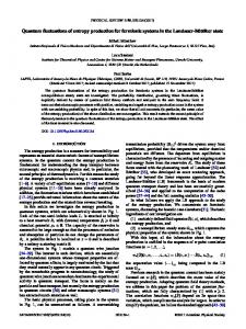
Figure 1. Pictorial representation of the reconstruction algorithm—the reconstruction algorithm starts by optimally choosing the parameters j Î {α, β, γ} as the zeros of the Chebyshev polynomial of degree N in the intervals [jmin, jmax]. Then, the moment generating functions χC(j), with C Î{A, B, A−B}, are measured. The experimental steps for their measuring and a detail analysis ~ about the required number of measurements to perform the procedure are explained in the main text. Once the estimates ás Ck ñ of the 1 statistical moments of σC are obtained, the inverse Fourier transform has to be numerically performed. Alternatively, the Moore– Penrose pseudo-inverse of ΣC can be adopted. As a result, an estimate Prob (sC ) for the probability distribution Prob(σC) is obtained.
~ chosen number N of extracted moments. As a matter of fact, each statistical moment ás Ck ñ, with C Î{A, B, A−B}, is the best approximation of the true statistical moments of σC from the measurement of the corresponding characteristic functions χC(j). Hence, apart from a numerical error coming from the inversion of the Vandermonde matrix A or the use of the Newton polynomials cCpol , we can state that ~ ás Ckñ
MC
å sCk ,i Prob(sC,i) = sCk,1 Prob(sC,1) + ¼ + sCk ,M
C
i=1
Prob (sC, MC ) ,
(54)
with k=1, K, N. In equation (54), MC is equal to the number of values that can be assumed by σC, while σC,i denotes the ith possible value for the stochastic quantum entropy production of the (sub)system C. As a result, the probabilities Prob(σC, i), i=1, K, M, can be approximately expressed as a function of the statistical ~ moments {ás Ck ñ}, i.e. ⎛~ ⎞ ⎛ sC,1 sC,2 ¼ sC, M ⎞ ⎛ Prob (sC,1) ⎞ ⎜ ásCñ ⎟ ⎜ 2 ⎟ ⎜ ~2 ⎟ s s 2 ¼ s C2 , M ⎟ ⎜ Prob (sC,2) ⎟ ⎜ ⎟, ⎜ ásC ñ ⎟ = ⎜ C,1 C,2 (55) ⎜ ⎟ ⎟⎜ ⎜ ⎟ ⎜ ⎟ ⎜ ⎟ M M M ⎜⎜~N ⎟⎟ ⎝ s C,1 s C,2 ¼ s C, N ⎠ ⎝ Prob (sC, M )⎠ ⎝ásC ñ⎠ SC
N ´ M . By construction ΣC is a rectangular matrix, that is computed by starting from the
where SC Î knowledge of the values assumed by the stochastic quantum entropy production σC,i. Finally, in order to obtain the probabilities Prob(σC,i), i=1, K, MC, we have to adopt the Moore–Penrose pseudo-inverse of ΣC, which is defined as SC+ º (STC SC )-1STC .
(56)
A pictorial representation of the reconstruction protocol is shown in figure 1. Let us observe, again, that the proposed algorithm is based on the expression of equation (14) for the stochastic quantum entropy production, which has been obtained by assuming unital CPTP quantum maps for the system dynamics. We expect that for a general open quantum system, not necessarily described by a unital CPTP map, one can extend the proposed reconstruction protocol, even though possibly at the price of a greater number of measurements. Notice that, since equation (13) it is not longer valid in the general case, one has to use directly equations (10)–(11). However, we observe that, as shown in [41], the ratio between the conditional probabilities may admit for a large family of CPTP maps the form p (akfin∣amin ) p (amin∣akref ) º e-DV , where the quantity ΔV is related to the so-called nonequilibrium potential, so that σ=σunital+V and σunital again given by equation (14). 5.1. Required number of measurements From an operational point of view, we need to measure (directly or indirectly) the quantities ⎧ c (a) = Tr{[(r )a Ä B] F [(r )1 - a Ä r ]} A A, t A,in B,in ⎪ b 1 ⎨ cB (b ) = Tr{[ A Ä (rB, t ) ] F [rA,in Ä (rB,in) - b ]} ⎪ ⎩ c A- B (g ) = Tr{(rt )g F [(r in)1 - g ]},
13
(57)
Quantum Sci. Technol. 3 (2018) 035013
S Gherardini et al
i.e. the moment generating functions of σA, σB and σA−B, after a proper choice of the parameters α, β and γ, with a, b , g Î . The optimal choice for these parameters was analyzed in the previous section. For this purpose, as shown in appendix D, it is worth mentioning that (rC ,in )1 - j º åm PCin, m p (xmin )1 - j and (rC , t )j º åk PCt , k p (xkt )j , where C Î{A, B, A−B}, x Î {a, b, c} and j Î {α, β, γ}. A direct measurement of χC(j), based for example on an interferometric setting as shown in [57, 58] for the work distribution inference, is not trivial, especially for the general fully quantum case. For this reason, we propose a procedure, suitable for experimental implementation, requiring a limited number of measurements, based on the following steps: (i) Prepare the initial product state rin = rA,in Ä rB,in , as given in equation (23), with fixed probabilities p (amin ) and p (bhin ). Then, after the composite system A−B is evolved within the time interval [0, τ], measure the occupation probabilities p (akfin ) and p (blfin ) via local measurements on A and B. Then, compute the stochastic quantum entropy productions sA (amin, akfin ) and sB (bhin, blfin ). Simultaneous in measurements on A and B yield also the probabilities p (cklfin ) and thus sA - B (cmh , cklfin ). (ii) For every chosen value of α, β and γ, prepare, for instance by quantum optimal control tools [83], the quantum subsystems in the states
⎧ ⎪ r IN (a) º ⎪ ⎪ ⎪ ⎨ r IN (b ) º ⎪ ⎪ ⎪ r (g ) º IN ⎪ ⎩
[(rA,in)1 - a Ä rB,in] Tr[(rA,in)1 - a Ä rB,in] [rA,in Ä (rB,in)1 - b ] Tr[rA,in Ä (rB,in)1 - b ]
,
(rA,in Ä rB,in)1 - g Tr[(rA,in Ä rB,in)1 - g ]
and let the system evolve. (iii) Since the characteristic function χC(j), with C Î{A, B, A−B} and j Î{α, β, γ}, is given by performing a trace operation with respect to the composite system A−B, one can write the following simplified relation: cC (j) =
å å ám∣ p (xkfin)j ∣kñák∣r FIN (j)∣mñ = å p (xmfin)j ám∣r FIN (j)∣mñ , k
m
(58)
m
where {∣lñ}, l=m, k, is the orthonormal basis of the composite system A−B, x Î{a, b, c} and ρFIN(j)≡Φ[ρIN(j)] (with p (xmfin ) measured in step 1 and ρIN(j) introduced in step 2). Thus, measure the occupation probabilities ám∣r FIN (j )∣mñ in order to obtain all the characteristic functions χC(j). We observe that the measure of the characteristic functions χC(j) relies only on the measure of occupation probabilities. Hence, the proposed procedure does not require any tomographic measurement. Moreover, for the three steps of the protocol we can well quantify the required number of measurements to properly infer the statistics of the quantum entropy production regarding the composite quantum system. The required number of measurements, indeed, scales linearly with the number of possible measurement outcomes coming from each quantum subsystem at the initial and final stages of the protocol. Equivalently, if we define dA and dB as the dimension of the Hilbert space concerning the quantum subsystems A and B, we can state that the number of measurements for both of the three steps scales linearly with (dA+dB), i.e. with the number of values (MA+MB) that can be assumed by σA and σB, the stochastic quantum entropy production of the subsystems. It also scale linearly with MA MB for the reconstruction of the stochastic quantum entropy production σA−B of the composite system. The reason is that the described procedure is able to reconstruct the distribution of the stochastic quantum entropy production, without directly measuring the joint probabilities pa(k, m) and pb(l, h) for the two subsystems and pc(mh, kl) for the composite system. Otherwise, the number of required measurements would scale, respectively, as MA2 and MB2 for the subsystems and as (MA MB )2 for the composite system in order to realize all the combinatorics concerning the measurement outcomes.
6. A physical example In the previous section, we have introduced an algorithm for the reconstruction of thermodynamical quantities in a fully quantum regime. Here, in order to illustrate our theoretical results, we discuss in this section an experimental implementation with trapped ions. Trapped ions have been demonstrated to be a versatile tool for quantum simulation [84–87], including simulation of quantum thermodynamics [20, 21, 43, 44, 88]. The application of our protocol on a physical example relies on the availability of experimental procedures for state preparation and readout, as well as an entangling operation. 14
Quantum Sci. Technol. 3 (2018) 035013
S Gherardini et al
Figure 2. Experimental implementation with trapped ions—pictorial representation of two trapped ions subjected to two laser fields. The internal levels of the ions allow to encode one qubit in each ion. The transition between these levels is driven by the lasers, where the driving depends on the state of the common vibrational (trap) mode of the two ions. The lasers can be focused to choose between single or global addressing. This allows to generate local gates as well as entangling gates.
We consider a system of two trapped ions, whose two internal states allow to encode the qubit states ∣0ñ and ∣1ñ of the standard computational basis. Then, the subsystems A and B are represented by the two qubits. The latter can interact by the common vibrational (trap) mode of the two ions, and external lasers allow to manipulate the ion states, generating arbitrary single qubit rotations through individual addressing or an entangling operation, as for example the Mølmer–Sørensen gate operation [89–92]. Figure 2 shows a pictorial representation of the system. While usually universal state preparation for single qubits is supposed only for pure states, here we have to prepare mixed states. However, once we have prepared a pure state with the right amount of population in the two levels, we can reach the required mixed state by applying a random Z rotation leading to a complete dephasing of the two levels, where Z is the corresponding Pauli matrix. The two-qubit operation, that generates entanglement between A and B, is chosen to be a partial Mølmer–Sørensen gate operation, given by the following unitary operation, depending on the phase f: (f) = e-if (X
A Ä XB)
,
(59)
where X A and X B equal, respectively, to the Pauli matrix X for the quantum systems A and B, and the reduced p Planckʼs constant is set to unity. In the following (and unless explicitly stated otherwise), we choose f = 7 ,
(
6
9
4
6
)
and start from the initial state r0 = diag 25 , 25 , 25 , 25 since this choice leads to a non-Gaussian probability distribution Prob(σA−B) of the stochastic quantum entropy production. For the sake of simplicity, we remove the label A and B from the computational basis {∣0ñ, ∣1ñ} considered for the two subsystems. Thus, the corresponding projectors are P0 º ∣0ñá0∣ and P1 º ∣1ñá1∣, and each ion is characterized by 4 different values of the stochastic quantum entropy production σC, with C Î{A, B}. As a consequence, the probability distribution Prob(σA−B) of the stochastic quantum entropy production for the composite system A−B is defined over a discrete support given by l samples, with l MA MB = 16. 6.1. Correlated measurement outcomes and correlations witness In the general case, the outcomes of the second measurement of the protocol are correlated, as in our example, and the stochastic quantum entropy production of the composite system is sub-additive, i.e. ásA - Bñ ásAñ + ásBñ. Hence, by adopting the reconstruction algorithm proposed in figure 1 we are able to effectively derive the upper bound of ásA - Bñ, which defines the thermodynamic irreversibility for the quantum process. In the simulations of this section, we compare the fluctuation profile that we have derived by performing local measurements on the subsystems A and B with the ones that are obtained via a global measurement on the composite system A−B, in order to establish the amount of information which is carried by a set of local measurements. Furthermore, we will discuss the changes of the fluctuation profile of the stochastic quantum entropy production both for unitary and noisy dynamics. The unitary operation describing the dynamics of the quantum system is given by equation (59), while the noisy dynamics can be described by the differential Lindblad (Markovian) equation r˙ (t ) = (r (t )), defined as 15
Quantum Sci. Technol. 3 (2018) 035013
S Gherardini et al
Figure 3. Statistical moments of σA−B and σA+B as a function of the phase f with unitary dynamics—in the four top panels, the statistical moments ás kA - Bñ and ás kA + Bñ, k=1, K, 4, of the stochastic quantum entropy production σA−B and σA+B as a function of f Î[0, 2π] are shown, in the case the dynamics of the composite quantum system A−B is unitary. In the two bottom panels, moreover, we plot a comparison between the samples of the probability distributions Prob(σA−B), Prob(σA+B) (black squares) and the samples of the corresponding reconstructed distribution (red circles). The latter numerical simulations are performed by considering f=π/7, and N equals, respectively, to 20 (for the fluctuation profile of σA−B) and 10.
å
r˙ (t ) = - i [H , r ] -
C Î {A, B}
GC ({r , LC† LC} - 2LC rLC†).
(60)
In equation (60), ρ(t) denotes the density matrix describing the composite quantum system A−B, {·, ·} is the anticommutator, ΓA and ΓB (rad s−1) are dephasing rates corresponding to LA º P0 Ä B and LB º A Ä P0 , pure-dephasing Lindblad operators, where A and B are the identity operators acting, respectively, on the Hilbert spaces of the ions A and B. The Hamiltonian of the composite system A−B in equation (60), instead, is given by
H = w (X A Ä X B ) , where the interaction strength ω=f/τ (rad s−1) with τ kept fixed and chosen equal to 50 s (leading to a largely relaxed system dynamics), consistently with the unitary operation (59). In figures 3 and 4, we plot the first 4 statistical moments of σA−B and σA+B as a function of the phase f, respectively, in case of unitary and noisy dynamics. Moreover, we show, for a given value of f, the probability distributions Prob(σA−B) and Prob(σA+B) for both unitary and noisy dynamics, compared with the corresponding reconstructed distributions obtained by applying the reconstruction algorithm, which we call Prob (sA - B ) and Prob (sA + B ), respectively. Let us recall that Prob(σA+B) is obtained by performing the two local fin measurements with observables fin A and B independently (disregarding the correlations of their outcomes) fin on the subsystems A, B, while the distribution Prob(σA−B) requires to measure fin A and B simultaneously, i.e. fin measuring the observable A - B , defined by equation (27). For unitary dynamics, the statistical moments of the stochastic quantum entropy productions σA−B and σA+B follow the oscillations of the dynamics induced by changing the gate phase f. Conversely, for the noisy dynamics of equation (60), with Γ=ΓA=ΓB different from zero, when f increases the system approaches a fixed point of the dynamics. Consequently, the statistical moments of the stochastic quantum entropy production tend to the constant values corresponding to the fixed point, and the distribution of the stochastic entropy production becomes narrower. In both figures 3 and 4, the first statistical moments (or mean values) ásA - Bñ and ásA + Bñ are almost overlapping, and the sub-additivity of σA−B is confirmed by the numerical simulations. Furthermore, quite surprisingly, also the second statistical moments of σA−B and σA+B are very similar to each other. This means that the fluctuation profile of the 16
Quantum Sci. Technol. 3 (2018) 035013
S Gherardini et al
Figure 4. Statistical moments of σA−B and σA+B as a function of the phase f with noisy dynamics—in the four top panels, the statistical moments ás kA - Bñ and ás kA + Bñ, k=1, K, 4, of the stochastic quantum entropy production σA−B and σA+B as a function of f Î[0, 2π] are shown, in the case the dynamics of the composite quantum system A−B is described by a Lindblad (Markovian) equation. In the two bottom panels, moreover, we plot a comparison between the samples of the probability distributions Prob(σA−B), Prob(σA+B) (black squares) and the samples of the corresponding reconstructed distribution (red circles). The latter numerical simulations are 5p performed by considering f = 6 , Γ=ΓA=ΓB=0.2 rad s−1, and N equals, respectively, to 20 (for the fluctuation profile of σA−B) and 10.
stochastic entropy production σA+B is able to well reproduce the probability distribution of σA−B in its Gaussian approximation, i.e. according to the corresponding first and second statistical moments. In addition, we can state that the difference of the higher order moments of ásA + Bñ and ásA - Bñ reflects the presence of correlations between A and B created by the map, since for a product state σA−B=σA+B. Therefore, the difference between the fluctuation profiles of σA−B and σA+B constitutes a witness for classical and/or quantum correlations in the final state of the system before the second measurement. As a consequence, if Prob(σA−B) and Prob(σA+B) are not identically equal, then the final density matrix ρfin is not a product state, and (classical and/or quantum) correlations are surely present. Notice that the converse statement is not necessarily true because the quantum correlations can be partially or fully destroyed by the second local measurements, while the classical ones are still preserved and so detectable. In figure 5 the first 4 statistical moments of σA−B and σA+B are shown as a function of Γ (rad s−1). As before, we can observe a perfect correspondence between the two quantities when we consider only the first and second statistical moments of the stochastic quantum entropy productions, and, in addition, similar behavior for the third and fourth statistical moments. Indeed, since the coherence terms of the density matrix describing the dynamics of the composite quantum system tend to zero for increasing Γ, the number of samples of σA−B and σA+B with an almost zero probability to occur is larger, and also the corresponding probability distribution approaches to a Gaussian one, with zero mean and small variance. In accordance with figures 3 and 4, this result confirms the dominance of decoherence in the quantum system dynamics, which coincides with no creation of correlations. In the following subsection, we will evaluate the performance of the proposed reconstruction algorithm for the reconstruction of Prob(σA) and Prob(σB). This choice is largely justified also by the possibility to characterize the irreversibility of an arbitrary quantum process, given by the mean value of the stochastic quantum entropy production σA−B, via the reconstruction of the corresponding upper bound in accordance with the sub17
Quantum Sci. Technol. 3 (2018) 035013
S Gherardini et al
Figure 5. Statistical moments of σA−B and σA+B as a function of the dephasing rate Γ—the statistical moments ás kA - Bñ and ás kA + Bñ, k=1, K, 4, of the stochastic quantum entropy production σA−B and σA+B as a function of Γ Î [0, 1.2] rad s−1 are shown, in the case the dynamics of the composite quantum system A−B is described by a Lindblad (Markovian) equation, with f=π/7.
additivity property. Still, a similar behavior was found for the probability distribution Prob(σA−B) of the stochastic quantum entropy production of the composite system. 6.2. Reconstruction for unitary dynamics In this section, we show the performance of the reconstruction algorithm for the probability distribution of the stochastic quantum entropy production σA+B via local measurements on the subsystems A and B, when the dynamics of the quantum system is unitary. In particular, in the numerical simulations, we take the parameters α and β of the algorithm, respectively, equal to the real zeros of the Chebyshev polynomial of degree N in the intervals [amin , amax ] = [0, N ] and [bmin, bmax ] = [0, N ]. This choice for the minimum and maximum values of the parameters α and β ensures a very small numerical error (about 10−4) in the evaluation of each statistical moment of σA and σB via the inversion of the Vandermonde matrix, already for N>2. Indeed, since all the elements of the vectors a and b are different from each other, i.e. ai ¹ aj and bi ¹ bj " i , j = 1, ¼, N , we can derive the statistical moments of σC, with C Î {A, B}, by inverting the corresponding Vandermonde matrix. The number N of evaluations of the moment generating functions χA(α) and χB(β), instead, has been taken as a free parameter in the numerics in order to analyze the performance of the reconstruction algorithm. The latter may be quantified in terms of the root mean square error(RMSE) defined as
å k = 1 ∣ás kA+ Bñ - ás kA+ Bñ∣2 , Nmax
RMSE ({ás kA+ Bñ }kN=max1 )
º
Nmax
where {ás kA + Bñ} are the true statistical moments of the stochastic quantum entropy production σA+B, which have been numerically computed by directly using equations (33)–(35), while ás kA + Bñ are the reconstructed 18
(61)
Quantum Sci. Technol. 3 (2018) 035013
S Gherardini et al
Figure 6. Reconstructed statistical moments of σA, σB and σA+B as a function of N with unitary dynamics—in the four top panels we show the statistical moments ás Ck ñ, C={A, B} (equal due to symmetry), and ás kA + Bñ, k=1, K, 4, of the stochastic quantum entropy production σA, σB and σA+B as a function of N. As N increases, the reconstructed statistical moments converge to the corresponding true value. The corresponding RMSEs RMSE ({ás kA + Bñ}) and RMSE ({Prob (sA + B, i )}), instead, are plotted in the two bottom panels. All the numerical simulations in the figure are performed by considering unitary dynamics for the composite system A−B with f=π/7.
statistical moments after the application of the inverse Fourier transform or the Moore–Penrose pseudo-inverse of ΣC, C Î{A, B}. Nmax, instead, is the largest value of N considered for the computation of the RMSE ({ás kA + Bñ}) in the numerical simulations (in this example Nmax=16). Another measure for the evaluation of the algorithm performance, which will be used hereafter, is given by the RMSE
å i= 1Ri2 , l
RMSE ({Prob (sA+ B, i )}li = 1 ) º
l
(62)
where R i º ∣Prob (sA + B, i ) - Prob (sA + B, i )∣ is the reconstruction deviation, i.e. the discrepancy between the true and the reconstructed probability distribution Prob(σA+B). The RMSE ({Prob (sA + B, i )}) is computed with respect to the reconstructed values Prob (sA + B, i ) of the probabilities Prob(σA+B, i), i=1, K, l, for the stochastic quantum entropy production σA+B. Figure 6 shows the performance of the reconstruction algorithm as a function of N for the proposed experimental implementation with trapped ions in case the system dynamics undergoes a unitary evolution. In particular, we show the first 4 statistical moments of σA, σB and σA+B as a function of N. Let us observe that the statistical moments of the stochastic quantum entropy production of the two subsystems A and B are equal due to the symmetric structure of the composite system. As expected, when N increases, the reconstructed statistical moments converge to the corresponding true values, and also the reconstruction deviation tends to zero. This result is encoded in the RMSEs of equations (61)–(62), which behave as monotonically decreasing functions. Both the RMSE ({ás kA + Bñ}) and RMSE ({Prob (sA + B, i )}) sharply decrease for about N 6, implying that the reconstructed probability distribution Prob (sA + B ) overlaps with the true distribution Prob(σA+B) with very small reconstruction deviations Ri. Since the system of two trapped ions of this example is a small size system, we have chosen to derive the probabilities {Prob(σA,i)} and {Prob(σB,i)}, i=1, K, 4, without performing the ~ inverse Fourier transform on the statistical moments {ás Ck ñ}, C Î{A, B}. Indeed, the computation of the inverse Fourier transform, which has to be performed numerically, can be a tricky step of the reconstruction procedure, because it can require the adoption of numerical methods with an adaptive step-size in order to solve the numerical integration. In this way, the only source of error in the reconstruction procedure is given by the 19
Quantum Sci. Technol. 3 (2018) 035013
S Gherardini et al
Figure 7. True and reconstructed statistical moments of σA, σB and σA+B as a function of the phase f with unitary dynamics—the statistical moments ás Ck ñ, C={A, B} (equal by symmetry), and ás kA + Bñ, k=1, K, 4, of the stochastic quantum entropy production σA, σB and σA+B are shown as a function of the phase f. All the numerical simulations are performed by considering unitary dynamics for the composite system A−B with N=10 and f Î[0, 2π].
expansion in Taylor series of the quantity χC(j), with C Î{A, B} and j Î{α, β}, around j=0 as a function of a finite number of statistical moments ás Ck ñ, k=1, K, N−1. As shown in figure 6, the choice of the value of N is a degree of freedom of the algorithm, and it strictly depends on the physical implementation of the reconstruction protocol. In the experimental implementation above with two trapped ions, N=10 ensures very good performance without making a larger number of measurements with respect to the number of values assumed by the stochastic quantum entropy production σA+B. In figure 7, moreover, we show for N=10 the first 4 true statistical moments of the stochastic quantum entropy productions σA and σB of the two subsystems, as well as the correlation-free convolution σA+B as a function of f Î[0, 2π], along with the corresponding reconstructed counterpart ás Ck ñ, k=1, K, 4, C Î{A, B, A+B}. As before, the reconstruction procedure yields values very close to the true statistical moments of σA, σB and σA+B for all values of the phase f. 6.3. Reconstruction for noisy dynamics Here, the performance of the reconstruction algorithm is discussed in case the system dynamics is affected by pure-dephasing contributions, described via the differential Lindblad (Markovian) equation r˙ (t ) = (r (t )), given by equation (60). The Hamiltonian of the composite system A−B is defined as H = w (X A Ä XB ). Since the fixed duration τ of the transformation has been chosen as before equal to 50 s, we choose the desired phase f by setting the interaction strength to ω ≡ f/τ (rad s−1). Figure 8 shows the RMSE ({ás kA + Bñ}) computed from the reconstructed statistical moments of the stochastic quantum entropy production σA+B. As it can be observed, apart from an initial transient, the mean error monotonically tends to zero as N increases, similarly to the case of unitary dynamics (see figure 6), such that it can be considered sufficiently small for N>8. Again, we evaluate the performance of the reconstruction algorithm also as a function of the phase f=ωτ, with τ fixed. As shown in figure 9, when f increases (with a fixed value of Γ, set to 0.2 rad s−1) the statistical moments of σA+B (but not necessarily the ones regarding the subsystems A and B) increase as well, since when f increases the system tends to a fixed point of the dynamics. Also the reconstruction procedure turns out to be more accurate for larger values of f, as shown in the two bottom panels of figure 9 (for this figure we use the Fourier transform). The reason is that when the dynamics 20
Quantum Sci. Technol. 3 (2018) 035013
S Gherardini et al
Figure 8. RMSE from the reconstructed statistical moments as a function of N—root mean square error RMSE ({ás kA + Bñ}) as a function of N. All the numerical simulations are performed by considering a Lindblad (Markovian) dynamics for the composite system A−B, given by equation (60), where the dephasing rates Γ=ΓA=ΓB are chosen equal to 0.2 rad s−1, and f=π/7.
Figure 9. True and reconstructed statistical moments of σA, σB and σA+B as a function of the phase f with noisy dynamics—in the first 4 panels the statistical moments ás Ck ñ, C={A, B} (equal by symmetry), and ás kA + Bñ, k=1, K, 4, of the stochastic quantum entropy production σA, σB and σA+B are shown as a function of the phase f. All the numerical simulations are performed by considering a Lindblad (Markovian) dynamics for the composite system A−B, given by equation (60), with N=10, Γ=0.2 rad s−1, and f Î[0, 2π]. In the bottom panels of the figure, instead, we show the root mean square errors RMSE ({ás kA + Bñ}) and RMSE ({Prob (sA + B, i )}).
21
Quantum Sci. Technol. 3 (2018) 035013
S Gherardini et al
Figure 10. True and reconstructed statistical moments of σA, σB and σA+B as a function of the dephasing rate Γ—the first three statistical moments of the stochastic quantum entropy productions for A, B (equal by symmetry) and the composite system A−B as a function of the dephasing rate Γ=ΓA=ΓB (rad s−1) are shown for the physical example of 2 trapped ions. In particular, the statistical moments of σA+B are put beside their reconstructed version, which have been obtained by choosing N=10 and f=π/7. In the last panel, moreover, the corresponding root mean square error RMSE ({ás kA + Bñ}) as a function of Γ is shown.
approaches the fixed point, the distribution of the stochastic quantum entropy production becomes narrower and the convergence of the Fourier integral is ensured. Finally, in figure 10 we plot the behavior of the first three statistical moments of σA, σB and σA+B as a function of the dephasing rate Γ=ΓA=ΓB (rad s−1), with N=10 and f=π/7. As before, due to the symmetry of the bipartition, the statistical moments of σA and σB are identically equal. For increasing Γ the dephasing becomes dominant over the interaction and all correlations between the subsystems are destroyed. As a consequence, the stochastic quantum entropy production tends to zero as is observed in the figure for all the investigated moments, both for the subsystems and the composite system. 6.4. Probing irreversibility Once the fluctuation profile of the stochastic quantum entropy production (i.e. the corresponding probability distribution) is reconstructed, then the irreversibility properties of the composite system transformation can be successfully probed. The thermodynamic irreversibility, indeed, is quantified by means of the mean value ásA - Bñ, with ásA - Bñ = 0 corresponding to thermodynamic reversibility. As previously shown in figures 3–5, the mean value ásA - Bñ can be well approximated by ásA + Bñ and from equations (16) and (32) we have 0 ásA - Bñ ásA + Bñ. From figures 5 and 10, thus, we can observe that the implemented noisy transformation is more reversible with respect to the unitary one. Indeed, the statistical moments of the stochastic quantum entropy production, as well as the corresponding mean value, go to zero as Γ increases. Since the dynamics originating from the Lindblad equation (60) admits as a fixed point the completely mixed state of the composite system A−B, if we increase the value of Γ then the probability distribution of the quantum entropy production for the systems A, B and A−B tends to a Kronecker delta around zero, leading to a more reversible system transformation with respect to the unitary case. For this reason, also the numerical simulations of figure 10 have been performed by using the inverse Fourier transform to reconstruct the probabilities {Prob(σC,i)}, with i=1, 22
Quantum Sci. Technol. 3 (2018) 035013
S Gherardini et al
K, MC and C Î{A, B}, instead of calculating the pseudo-inverse of the matrix ΣC. As a matter of fact, as Γ increases some values of σC approach zero and ΣC becomes singular. Let us observe that when the dynamics is unitary the performance of the reconstruction algorithm adopting the inverse Fourier transform can be affected by a not-negligible error, as shown by the RMSE ({ás kA + Bñ}) in the last panel of figure 10. For such case, the adoption of the pseudo-inverse of ΣC is to be preferred. Moreover, we expect that increasing the number of ions the thermodynamic irreversibility becomes more and more pronounced and that this analysis may be the object of forthcoming work. In conclusion, a system transformation on a multipartite quantum system involves stochastic quantum entropy production whenever correlations between the subsystems of the multipartite system is first created by the dynamics of the composite system and then destroyed by the second measurement. This result, indeed, can be easily deduced from figures 9 and 10, in which, for a fixed value of Γ (Γ = 0.2 rad s−1) and f (f=π/7) respectively, the behavior of the statistical moments of the stochastic quantum entropy production as a function of f (Γ) is monotonically increasing (decreasing). Indeed, the stronger is the interaction between the two ions, the larger is the corresponding production of correlations between them. On the other side, instead, the production of correlations within a multipartite system is inhibited due to the presence of strong decoherent processes.
7. Discussion and conclusions The goal of this paper has been three-fold: We discussed how to relate the stochastic quantum entropy production to the quantum fluctuation theorem, which is the generalization of the Tasaki–Crooks theorem for open systems, and this relation is based on the evaluation and quantification of the irreversibility by means of a two-times measurement protocol. By using the definition of the stochastic quantum entropy production, then, we introduced a protocol to reconstruct its fluctuations, and characterize the dynamics of the quantum system. In particular, the proposed procedure allows us to determine the mean value ásñ of the stochastic quantum entropy production, quantifying and probing the amount of irreversibility, with ásñ = 0 (ásñ > 0) corresponding to thermodynamic reversibility (irreversibility). At variance, ásñ < 0—violating the second law of the thermodynamics—do not occur due to the non-negativity of the Kullback–Leibler divergence. Furthermore, we have shown the relation between the quantum relative entropy of the system density matrix at the final time of the transformation and the stochastic quantum entropy production. In this regard, equation (16) is valid also at zero temperature and without assuming thermal baths with finite temperature. It is worth noting, however, that the presented results about the stochastic quantum entropy production are based on the assumption to consider unital CPTP quantum maps for the description of the open system dynamics. Even though we limited ourself for most of the paper to unital CPTP quantum maps, in section 3.2 we discussed how to put in relation our results with the conventional second law of thermodynamics at finite temperature. Secondly to reconstruct the probability distribution of σ, we proposed a suitable reconstruction protocol based on the determination of the characteristic functions of the stochastic quantum entropy production, which are evaluated N times for a given set of N real parameters, so as to collect an adequate amount of information for the reconstruction. In other words, the reconstruction algorithm relies on a parametric version of the integral quantum fluctuation theorem, and yields the first N statistical moments of the stochastic quantum entropy production through the inversion of a Vandermonde matrix, which encodes the experimental evaluation of the characteristic function. The corresponding numerical error, however, can be reduced using the solution of a polynomial interpolation problem based on the use of (zeros of) the Chebyshev polynomials. Then, the presented algorithm in its generic form uses a numerical inverse Fourier transform to reconstruct the probability distribution of the stochastic quantum entropy production from its statistical moments. In order to optimize the minimum amount of resources needed for the protocol, we have also shown that the required number of measurements to perform the algorithm scales linearly with the number of the values that can be assumed by the stochastic quantum entropy production, and not quadratically as one would have obtained by a direct application of the definition of the corresponding probability distributions. Moreover, as third aspect, under the hypothesis that the open quantum system is composed by mutually interacting subsystems, we investigated the stochastic quantum entropy production both for the subsystems and for the composite system, showing that their mean values are sub-additive; they coincide only when the system density matrix at the end of the transformation is a product state. In this way, we have proved not only how to characterize the irreversibility of an arbitrary unital quantum process by reconstructing the corresponding upper bound in accordance with the sub-additivity, but we have also provided a method to detect correlations between the partitions of the system, just by comparing the fluctuation profiles of σA+B and σA−B. In this regard, let us recall that the correlation shared by two parts of a composite system (let us consider e.g. even just the 23
Quantum Sci. Technol. 3 (2018) 035013
S Gherardini et al
entanglement, genuinely quantum type of correlation) is not directly measurable in laboratory, since there does not exist a self-adjoint operator quantifying it. To this aim, one could perform a single quantum state tomography on the final state of the system after the transformation and evaluate the quantum discord for such state, so as to measure nonclassical correlations between its partitions [93]. However, it is worth noting that the performance of a full state tomography is not always feasible in terms of the available resources, and, along this direction, nontrivial solutions have been recently introduced (see e.g. [94]). Conversely, as previously shown, the measure of the probability distribution of the quantum entropy production by performing measurements both on local and global observables of the composite system does not require any quantum state tomography, since only measurements of the occupation probabilities of the final density matrix of the system are needed. Finally, to detect correlations one could also directly measure the second order dynamical correlation function of the system. However, such procedure, although it could not require a full quantum state tomography, is extremely system-dependent and usually a relevant experimental effort is necessary though, it has been recently introduced a measurement apparatus relying on weak-ancilla-system couplings, which could in part facilitate such measurements [95]. In order to illustrate our theoretical results, we discussed an experimental implementation with trapped ions and we showed the performance of the reconstruction algorithm on a quantum system composed of two trapped ions, subjected to a unitary evolution and to a Lindbladian one. We showed that the probability distribution of the stochastic quantum entropy production can be efficiently reconstructed with a very small error already with N=7 momenta. Efficiency and possible extensions of the presented procedure have been also discussed. Generalizations of our results to more general (non-unital) quantum maps have been briefly discussed and will be investigated in a future work. Our protocol, summarized in figure 1, is experimentally oriented and it is based on the preparation of suitably prepared initial states, depending on the parameter j entering the characteristic functions χC(j) to be measured. Such protocol appears to be within the reach of experimental realizations, given the remarkable results obtained in the last decades in the preparation of quantum states [96]. In this regard, we observe that state preparation can be achieved in most common quantum technology platforms via optimal control procedures [97], allowing to speed up the process of coherent population transfer up to the ultimate bound imposed by quantum mechanics, i.e. the quantum speed limit [83, 98]. As a final remark, we also observe that the fluctuation properties of the stochastic quantum entropy production do strongly depend on the presence of decoherent channels between an arbitrary quantum system and the environment. Hence, one could effectively determine not only the influence of the external noise sources on the system dynamics, but also characterize the environment structure and properties via quantum sensing procedures. We believe that this aspect could be the subject for future investigations, e.g. along the research direction proposed in [99, 100], based on stochastic quantum Zeno phenomena [101, 102], and/or in [103, 104] via engineered quantum networks.
Acknowledgments The authors gratefully acknowledge Mauro Paternostro, Giorgio Battistelli, Giacomo Gori, Jin Wang, Francesco Saverio Cataliotti, Duccio Fanelli, Pietro Silvi and Augusto Smerzi for useful discussions. SG and MMM thank the Scuola Internazionale Superiore di Studi Avanzati (SISSA), Trieste (Italy) for hospitality during the completion of this work. AT thanks the Galileo Galilei Institute for Theoretical Physics for the hospitality in the Workshop ‘From Static to Dynamical Gauge Fields with Ultracold Atoms’ and the INFN for partial support during the completion of this work. This work was financially supported from Fondazione CR Firenze through the project Q-BIOSCAN.
Appendix A. Proof of theorem 1 In this appendix, we prove the equality between the conditional probabilities p (akfin∣amin ) and p (amin∣akref ), respectively, of the forward and backward processes of our two-time measurement scheme. Let us recall the ~ ~ ~in ~ref in observables in º åm amin Pm , fin º åk akfin Pkfin , ref º åk akref Pk and in = åm amin Pm , as defined in the main text. The dynamical evolution of the open quantum system between the two measurements is described by a unital CPTP map F(·) (with F () = ), whose Kraus operators {Eu} are such that åu Eu† Eu = , where denotes the identity operator on the Hilbert space of the quantum system. Accordingly, F (rin, m) = åu Eu rin, mEu†, in in where rin, m º Pm , and thus the conditional probability p (akfin∣amin ) equals to r0 P m 24
Quantum Sci. Technol. 3 (2018) 035013
S Gherardini et al
p (akfin∣amin) =
Tr[Pkfin F (r in, m)] in in Tr[Pm ] r 0 Pm
=å
=
† Tr[Pfin k å u E u r in, mEu ] in in Tr[Pm ] r 0 Pm
in in † Tr[Pfin k E u Pm r 0 Pm Eu ]
u
in in Tr[Pm ] r 0 Pm
=
å ∣áfa ∣Eu∣ya k
ñ ∣2 .
m
(A.1)
u
Next, by inserting in equation (A.1) the identity operator = QQ† = Q†Q, where Θ is the time-reversal operator as defined in the main text, one has: ∣QEu Q†∣~ ∣ áfak∣Eu∣yamñ ∣2 = ∣ áfak∣Q† (QEu Q†) Q∣yamñ ∣2 = ∣ áf yamñ ∣2 ak ~ ñ ∣2 , = ∣ áyam∣QEu† Q†∣f ak
(A.2)
where we have used complex conjugation and the modulus squared to flip the order of the operators. The timereversal of a single Kraus operator is Eu º p1 2Eu† p-1 2†, where we choose = Q and p = (as Φ is unital, such that F () = ). We can now state that ~ ñ ∣2 . ∣ áfak∣Eu∣yamñ ∣2 = ∣ áyam∣Eu∣f (A.3) ak Moreover, by observing that ~in Tr[Pm F (rref, k)] ~ 2 å ∣áyam∣Eu∣fakñ ∣ = ~ref ~ref = p (amin∣akref ) , u Tr[Pk rt Pm ]
(A.4)
~ref ~ref where rref, k º Pk rt Pm , the equality p (akfin∣amin ) = p (amin∣akref ), as well as the theorem 1, follow straightforwardly.
Appendix B. Proof of theorem 2 Here, we prove theorem 2, i.e. the inequality
0 S (r fin rt ) ásñ , where ρfin and ρτ are the density operators of the open quantum system before and after the second measurement of the forward process. S(ρfinPρτ) is called the quantum relative entropy of ρfin and ρτ and ásñ is the average of the stochastic quantum entropy production. This inequality may be regarded as the quantum counterpart of the second law of thermodynamics for an open quantum system. ⎡ p (ain) ⎤ Let us consider the stochastic entropy production s (afin, ain ) = ln ⎢⎣ p (aref ) ⎥⎦ (as given in equation (14) in the main text) for the open quantum system , whose validity is subordinated to the assumptions of theorem 1. Accordingly, the average value of σ is ás ñ =
⎡ p (a in) ⎤ p (afin , a in) ln ⎢ ⎥= ⎣ p (aref ) ⎦ a fin, a in
å
å p (ain) ln[ p (ain)] - å p (afin) ln[ p (aref )] 0. a in
(B.1)
a fin
We observe that the mean quantum entropy production ásñ is a non-negative quantity due to the positivity of the classical relative entropy, or Kullback–Leibler divergence. Since p (afin ) º áfa∣rfin∣fañ and the reference state is diagonal in the basis {∣fañ}, we have
å p (afin) ln[ p (aref )] = å áfa∣r fin∣fañ ln[ p (aref )] = å áfa∣r fin ln rref ∣fañ = Tr[r fin ln rt ] , a fin
a fin
(B.2)
a fin
where the last identity is verified by assuming the equality between the reference state ρref and the density operator ρτ after the second measurement of the protocol. One also has:
å p (ain) ln[ p (ain)] = Tr[rin ln rin] = -S (rin) ,
(B.3)
a in
where S (rin ) º -Tr [rin ln rin] is the von Neumann entropy for the initial density operator ρin of the quantum system . The mean quantum entropy production ásñ, thus, can be written in general as ásñ = - Tr [r fin ln rt ] - S (r in).
(B.4)
The quantum relative entropy is defined as S (rfin rt ) = -Tr [rfin ln rt ] - S (rfin ) and trivially S (rfin rt ) 0. According to our protocol, the initial and the final states are connected by the unital CPTP map Φ as ρfin=Φ(ρin). As a consequence of the unitality of Φ the von Neumann entropies obey the relation S (rin ) S (rfin ) [52]. Summarizing, we obtain 0 S (r fin rt ) = - Tr[r fin ln rt ] - S (r fin) - Tr[r fin ln rt ] - S (r in) = ásñ ,
proving the original inequality. 25
(B.5)
Quantum Sci. Technol. 3 (2018) 035013
S Gherardini et al
Note that if we perform the second measurement with a basis in which ρfin is diagonal (i.e. vanishing commutator between measurement operator and final state, [fin, rfin] = 0), the state is unchanged by the second measurement and ρfin=ρτ. As a consequence 0 = S (r fin rt ) ásñ = S (r fin) - S (r in) ,
i.e. the quantum relative entropy vanishes, while the average of the stochastic entropy production equals to the difference of final and initial von Neumann entropies, ásñ = S (rfin ) - S (rin ), and thus describes the irreversibility distribution of the map Φ only (and not of the measurement, as it would be in the general case). In the general case, i.e. if the condition [fin, rfin] = 0 does not hold, still the post-measurement state ρτ is diagonal in the basis of the observable eigenstates and we obtain ásñ = - Tr [r fin ln rt ] - S (r in) = S (rt ) - S (r in).
(B.6)
Appendix C. Recovering the second law of thermodynamics Here we show the formal derivation to connect the entropy production inequality in theorem 2 to the second law of thermodynamics for the open quantum system in term of the mean work áW ñ and the free-energy difference ΔF as defined in the main text. The main ingredient of this proof is to express Tr[ρfinlnρτ] as a function of the thermal state rtth º e b [F (t ) - H (t )] at time t=τ. In particular, we can write that Tr [r fin ln rt ] = Tr [r fin ln rtth] + Tr [r fin ln rt ] - Tr [r fin ln rtth] = Tr [r fin ln rtth] + Tr [r fin (ln r fin - ln r fin + ln rt - ln rtth)] = Tr [r fin ln rtth] + Tr [r fin (ln r fin - ln rtth)] - Tr [r fin (ln r fin - ln rt )] ,
so as to obtain Tr [r fin ln rt ] = Tr [r fin ln rtth] + S (r fin rtth) - S (r fin rt ) ,
(C.1)
i.e. equation (20) in the main text. Therefore, by taking equation (19) and substituting S (r in) = - Tr [r in ln r in] = - bF (0) + b Tr[r in H (0)]
with rin º e b [F (0) - H (0)], one has ásñ = bF (0) - b Tr[r in H (0)] - bF (t ) + b Tr[r fin H (t )] - S (r fin rtth) + S (r fin rt ).
Accordingly, being 0 S (rfin rt ) ásñ (from the results of theorems 1 and 2) and S (rfin rtth ) 0 (nonnegativity of the quantum relative entropy), we finally recover the conventional second law of thermodynamics, i.e. áW ñ DF .
Appendix D. Derivation of the characteristic functions In this appendix, we derive the expressions for the characteristic functions GA(λ) (for the probability distributions Prob(σA)) and GB(λ) (for the probability distributions Prob(σB)), given by equations (43) and (45), respectively. We start with the definition GA (l) =
ò ProbA (sA) e ils dsA, A
(D.1)
where Prob (sA) =
å d [sA - sA (amin, akfin)] pa (k, m) ,
(D.2)
k, m
as well as in pa (k , m) = Tr[(PtA, k Ä B) F (Pin A, m Ä r B,in)] p (am ) ,
(D.3)
sA (amin , akfin) = ln [ p (amin)] - ln [ p (akfin)].
(D.4)
and
26
Quantum Sci. Technol. 3 (2018) 035013
S Gherardini et al
Exploiting the linearity of Φ and the trace, we obtain GA (l) = å pa (k , m) e ilsA (am , ak in
fin
)
k, m
⎡⎛ ⎞ ⎛ ⎞⎤ fin il ln[ p (a min )] p (a in) Ä r ⎥ = Tr ⎢⎜å PtA, k e-il ln[ p (ak )] Ä B ⎟ F ⎜å Pin A, m e m B,in⎟ . ⎢⎣⎝ k ⎠ ⎝m ⎠ ⎥⎦
(D.5)
in Recalling the spectral decompositions of the initial and final density operators, rA,in º åm Pin A, m p (am ) and rA, t º åk PtA, k p (akt ), with eigenvalues p (amin ) and p (akt ) = p (akfin ), we get
å PtA,k e-il ln[ p (a
fin k )]
=
k
t k
å PtA,k e-il ln[ p (a )] = å PtA,k p (akt )-il = (rA,t )-il , k
(D.6)
k
and
å PinA,m e il ln[ p (a
in m )]
p (amin) =
m
å PinA,m p (amin)1 + il = (rA,in)1 + il .
(D.7)
m
If we insert these expressions into equation (D.5) we obtain the expression for the characteristic function GA(λ) given in equation (40). Analogously we can derive equation (41) for GB(λ). In a similar way we can derive the characteristic function GA−B(λ) of the stochastic entropy production of the composite system A−B: il 1 + il GA- B (l) = Tr[rt F (r in )].
ORCID iDs Filippo Caruso
https://orcid.org/0000-0002-8366-4296
References [1] [2] [3] [4] [5] [6] [7] [8] [9] [10] [11] [12] [13] [14] [15] [16] [17] [18] [19] [20] [21] [22] [23] [24] [25] [26] [27] [28] [29] [30] [31] [32] [33] [34] [35] [36] [37] [38] [39] [40]
de Groot S and Mazur P 1984 Non-Equilibrium Thermodynamics (New York: Dover) Jarzynski C 1997 Phys. Rev. Lett. 78 2690 Jarzynski C 2011 Annu. Rev. Condens. Matter Phys. 2 329–51 Crooks G 1999 Phys. Rev. E 60 2721 Hatano T and Sasa S 2001 Phys. Rev. Lett. 86 3463 Sakawa T and Ueda M 2010 Phys. Rev. Lett. 104 090602 Collin D, Ritort F, Jarzynski C, Smith S, Jr I T and Bustamante C 2005 Nature 437 231–4 Toyabe S, Ssagawa T, Ueda M, Muneyuki E and Sano M 2010 Nat. Phys. 6 988–92 Seifert U 2005 Phys. Rev. Lett. 95 040602 Tietz C, Schuler S, Speck T, Seifert U and Wrachtrup J 2006 Phys. Rev. Lett. 97 050602 Gemmer J, Michel M and Mahler G 2004 Quantum Thermodynamics (Berlin: Springer) Horodecki M and Oppenheim J 2013 Nat. Commun. 4 3059 Pekola J 2015 Nat. Phys. 11 118–23 Alhambra A, Masanes L, Oppenheim J and Perry C 2016 Phys. Rev. X 6 041017 Lostaglio M, Jennings D and Rudolph T 2015 Nat. Commun. 6 7383 Narasimhachar V and Gour G 2015 Nat. Commun. 6 8689 Lostaglio M, Korzekwa K, Jennings D and Rudolph T 2015 Phys. Rev. X 5 021001 Kammerlander P and Anders J 2016 Sci. Rep. 6 22174 Kim S, Sagawa T, Liberato S D and Ueda M 2011 Phys. Rev. Lett. 106 070401 Abah O, Roagel J, Jacob G, Deffner S, Schmidt-Kaler F, Singer K and Lutz E 2012 Phys. Rev. Lett. 109 203006 Roagel J, Abah O, Schmidt-Kaler F, Singer K and Lutz E 2014 Phys. Rev. Lett. 112 030602 Talkner P and Hänggi P 2016 Phys. Rev. E 93 022131 Campisi M, Talkner P and Hänggi P 2011 Phys. Rev. E 83 041114 Hekking F and Pekola J 2013 Phys. Rev. Lett. 111 093602 Venkatesh B P, Watanabe G and Talkner P 2015 New J. Phys. 17 075018 Alonso J, Lutz E and Romito A 2016 Phys. Rev. Lett. 116 080403 Deffner S, Paz J and Zurek W 2016 Phys. Rev. E 94 010103 Seifert U 2012 Rep. Prog. Phys. 75 126001 Esposito M, Harbola U and Mukamel S 2009 Rev. Mod. Phys. 81 1665 Campisi M, Hänggi P and Talkner P 2011 Rev. Mod. Phys. 83 771 Riera A, Gogolin C and Eisert J 2012 Phys. Rev. Lett. 108 080402 Gogolin C and Eisert J 2016 Rep. Prog. Phys. 79 056001 Kurchan J 2001 arXiv:cond-mat/0007360 Bunin G, D’Alessio L, Kafri Y and Polkovnikov A 2011 Nat. Phys. 7 913–7 Campisi M, Talkner P and Hänggi P 2009 Phys. Rev. Lett. 102 210401 Campisi M, Talkner P and Hänggi P 2010 Phys. Rev. Lett. 105 140601 Kafri D and Deffner S 2012 Phys. Rev. A 86 044302 Rastegin A 2013 J. Stat. Mech. 06 06016 Albash T, Lidar D, Marvian M and Zanardi P 2013 Phys. Rev. E 88 032146 Watanabe G, Venkatesh B P, Talkner P, Campisi M and Hänggi P 2014 Phys. Rev. E 89 032114
27
(D.8)
Quantum Sci. Technol. 3 (2018) 035013
[41] [42] [43] [44] [45] [46] [47] [48] [49] [50] [51] [52] [53] [54] [55] [56] [57] [58] [59] [60] [61] [62] [63] [64] [65] [66] [67] [68] [69] [70] [71] [72] [73] [74] [75] [76] [77] [78] [79] [80] [81] [82] [83] [84] [85] [86] [87] [88] [89] [90] [91] [92] [93] [94] [95] [96] [97] [98] [99] [100] [101] [102] [103] [104]
S Gherardini et al
Manzano G, Horowitz J and Parrondo J 2015 Phys. Rev. E 92 032129 Åberg J 2018 Phys. Rev. X 8 011019 Huber G, Schmidt-Kaler F, Deffner S and Lutz E 2008 Phys. Rev. Lett. 101 070403 An S, Zhang J N, Um M, Lv D, Lu Y, Zhang J, Yin Z Q, Quan H and Kim K 2014 Nat. Phys. 11 193–9 Mukamel S 2003 Phys. Rev. Lett. 90 170604 Cherniak V and Mukamel S 2004 Phys. Rev. Lett. 93 048302 Crooks G 2008 J. Stat. Mech. P10023 Deffner S and Lutz E 2011 Phys. Rev. Lett. 107 140404 Batalhao T, Souza A, Sarthour R, Oliveira I, Paternostro M, Lutz E and Serra R 2015 Phys. Rev. Lett. 115 190601 Brunelli M and Paternostro M 2016 arXiv:1610.01172 Frenzel M and Sagawa T 2016 arXiv:1609.08628 Sagawa T 2013 Lectures on Quantum Computing, Thermodynamics and Statistical Physics ed N Mikio et al (Singapore : World Scientific) Schmidt R, Maniscalco S and Ala-Nissila T 2016 Phys. Rev. A 94 010101(R) Koski J, Maisi V, Sagawa T and Pekola J 2014 Phys. Rev. Lett. 113 030601 Goold J, Huber M, Riera A, del Rio L and Skrzypczyk P 2016 J. Phys. A: Math. Theor. 49 143001 Camati P, Peterson J, Batalhao T, Micadei K, Souza A, Sarthour R, Oliveira I and Serra R 2016 Phys. Rev. Lett. 117 240502 Mazzola L, Chiara G D and Paternostro M 2013 Phys. Rev. Lett. 110 230602 Dorner R, Clark S, Heaney L, Fazio R, Goold J and Vedral V 2013 Phys. Rev. Lett. 110 230601 Goold J, Poschinger U and Modi K 2014 Phys. Rev. E 90 020101 Peterson J, Sarthour R, Souza A, Oliveira I, Goold J, Modi K, Soares-Pinto D and Cèleri L 2016 Proc. R. Soc. A 472 20150813 Liu F and Xi J 2016 Phys. Rev. E 94 062133 Campisi M, Blattmann R, Kohler S, Zueco D and Hänggi P 2014 New J. Phys. 15 105028 Fusco L, Pigeon S, Apollaro T, Xuereb A, Mazzola L, Campisi M, Ferraro A, Paternostro M and Chiara G D 2014 Phys. Rev. X 4 031029 Roncaglia A, Cerisola F and Paz J 2014 Phys. Rev. Lett. 113 250601 Nielsen M and Chuang I 2000 Quantum Computation and Quantum Information (Cambridge: Cambridge University Press) Breuer H and Petruccione F 2003 The Theory of Open Quantum Systems (Oxford: Oxford University Press) Caruso F, Giovannetti V, Lupo C and Mancini S 2014 Rev. Mod. Phys. 86 1203 Sozzi M 2008 Discrete Symmetries and CP Violation (Oxford: Oxford University Press) Crooks G 2008 Phys. Rev. A 77 034101 Horowitz J and Parrondo J 2013 New J. Phys. 15 085028 Cover T and Thomas J 2006 Elements of Information Theory (New Jersey: Wiley-Interscience) Umegaki H 1962 Phys. Rev. Lett. 14 59–85 Elouard C, Herrera-Martì D, Clusel M and Aufféves A 2017 NJP Quantum Inf. 3 9 Vedral V 2002 Rev. Mod. Phys. 74 197 Alicki R 1979 J. Phys. A: Math. Gen. 12 L103 Lorenzo S, McCloskey R, Ciccarello F, Paternostro M and Palma G 2015 Phys. Rev. Lett. 115 120403 Kallenberg O 2005 Probabilistic Symmetries and Invariance Principles (New York: Springer) Meyer C 2000 Matrix Analysis and Applied Linear Algebra (Philadelphia, PA: SIAM) Trefethen L 2000 Spectral Methods in MATLAB (Philadelphia, PA: SIAM) Phillips G 2003 Interpolation and Approximation by Polynomials (New York: Springer) Mnatsakanov 2008 Stat. Probab. Lett. 78 1869–77 Athanassoulis G and Gavriliadis P 2002 Probab. Eng. Mech. 17 273–91 Doria P, Calarco T and Montangero S 2011 Phys. Rev. Lett. 106 190501 Friedenauer A, Schmitz H, Glückert J, Porras D and Schätz T 2008 Nat. Phys. 4 757–61 Kim K, Chang M S, Korenblit S, Islam R, Edwards E, Freericks J, Lin G D, Duan L M and Monroe C 2010 Nature 465 590–3 Lanyon B et al 2011 Science 334 57–61 Gerritsma R, Kirchmair G, Zahringer F, Solano E, Blatt R and Roos C 2010 Nature 463 68–71 Roßnagel J, Dawkins S, Tolazzi K, Abah O, Lutz E, Schmidt-Kaler F and Singer K 2016 Science 352 325–9 Sørensen A and Mølmer K 1999 Phys. Rev. Lett. 82 1971–4 Roos C 2008 New J. Phys. 10 013002 Monz T, Schindler P, Barreiro J, Chwalla M, Nigg D, Coish W, Harlander M, Hänsel W, Hennrich M and Blatt R 2011 Phys. Rev. Lett. 106 130506 Nigg D, Müller M, Martinez E, Schindler P, Hennrich M, Monz T, Martin-Delgado M and Blatt R 2014 Science 345 302–5 Ollivier H and Zurek W 2001 Phys. Rev. Lett. 88 017901 Girolami D and Adesso G 2012 Phys. Rev. Lett. 108 150403 Uhrich P, Castrignano S, Uys H and Kastner M 2017 Phys. Rev. A 96 022127 Bergmann K, Theuer H and Shore B 1998 Rev. Mod. Phys. 70 1003 Brif C, Chakrabarti R and Rabitz H 2010 New J. Phys. 12 075008 Caneva T, Murphy M, Calarco T, Fazio R, Montangero S, Giovannetti V and Santoro G 2009 Phys. Rev. Lett. 103 240501 Müller M, Gherardini S and Caruso F 2016 Phys. Rev. A 94 042322 Müller M, Gherardini S and Caruso F 2016 Sci. Rep. 6 38650 Gherardini S, Gupta S, Cataliotti F, Smerzi A, Caruso F and Ruffo S 2016 New J. Phys. 18 013048 Müller M, Gherardini S and Caruso F 2017 Ann. Phys., Lpz. 529 1600206 Cosco F, Borrelli M, Plastina F and Maniscalco S 2017 Phys. Rev. A 95 053620 Nokkala J, Galve F, Zambrini R, Maniscalco S and Piilo J 2016 Sci. Rep. 6 26861
28