Reconstructing subsurface electrical wave orientation from cardiac epi-fluorescence recordings: Monte Carlo versus diffusion approximation Christopher J. Hyatt,1 Christian W. Zemlin,1 Rebecca M. Smith,1 Arvydas Matiukas,1,2 Arkady M. Pertsov,1 and Olivier Bernus 3,* 1
Department of Pharmacology, SUNY Upstate Medical University, 750 E Adams St, Syracuse, NY 13210, USA 2 Department of Physics, Kaunas University of Technology, Kaunas, Lithuania Institute of Membrane and Systems Biology, Faculty of Biological Sciences, University of Leeds, Leeds LS2 9JT, UK * Corresponding author:
[email protected]
3
Abstract: The development of voltage-sensitive dyes has revolutionized cardiac electrophysiology and made optical imaging of cardiac electrical activity possible. Photon diffusion models coupled to electrical excitation models have been successful in qualitatively predicting the shape of the optical action potential and its dependence on subsurface electrical wave orientation. However, the accuracy of the diffusion equation in the visible range, especially for thin tissue preparations, remains unclear. Here, we compare diffusion and Monte Carlo (MC) based models and we investigate the role of tissue thickness. All computational results are compared to experimental data obtained from intact guinea pig hearts. We show that the subsurface volume contributing to the epi-fluorescence signal extends deeper in the tissue when using MC models, resulting in longer optical upstroke durations which are in better agreement with experiments. The optical upstroke morphology, however, strongly correlates to the subsurface propagation direction independent of the model and is consistent with our experimental observations. ©2008 Optical Society of America OCIS codes: (170.3880) Medical and Biological Imaging; (170.3660) Light propagation in tissues
References and links 1. 2.
D. Streeter, Handbook of Physiology, (Bethesda, MD, American Physiological Society, 1979). R. A. Gray, A. M. Pertsov and J. Jalife, "Spatial and temporal organization during cardiac fibrillation," Nature 392, 75-78 (1998). 3. O. Bernus, M. Wellner and A. M. Pertsov, "Intramural wave propagation in cardiac tissue: asymptotic solutions and cusp waves," Phys. Rev. E 70, 061913 (2004). 4. F. Fenton and A. Karma, “Vortex dynamics in three-dimensional continuous myocardium with fiber rotation: Filament instability and fibrillation,” Chaos 8, 20-47 (1998). 5. K.H.J.W. Ten Tusscher, R. Hren and A.V. Panfilov, “Organization of ventricular fibrillation in the human heart,” Circ. Res. 100, e87-e101 (2007). 6. D. S. Rosenbaum and J. Jalife, Optical mapping of Cardiac excitation and arrhythmias, (Armonk, N Y, Futura Publishing Company, Inc. 2001). 7. I. R. Efimov, V. P. Nikolski and G. Salama, "Optical imaging of the heart," Circ. Res. 95, 21-33 (2004). 8. V. D. Khait, O. Bernus, S. Mironov and A. M. Pertsov, “Method for the three-dimensional localization of intramyocardial excitation centers using optical imaging,” J. Biomed. Opt. 11, 34007 (2006). 9. M. Wellner, O. Bernus, S. F. Mironov and A. M. Pertsov, “Multiplicative optical tomography of cardiac electrical activity,” Phys. Med. Biol. 51, 4429-46 (2006). 10. E. M. C. Hillman, O. Bernus, E. Pease, M. B. Bouchard and A. M. Pertsov, “Depth-resolved optical imaging of transmural electrical propagation in perfused heart,” Opt. Express 15, 17827-17841 (2007). 11. S. D. Girouard, K. R. Laurita, and D. S. Rosenbaum, "Unique properties of cardiac action potentials recorded with voltage-sensitive dyes," J. Cardiovasc. Electrophysiol. 7, 1024–1038 (1996). 12. W. Baxter, S. F. Mironov, A. V. Zaitsev, A. M. Pertsov and J. Jalife, "Visualizing excitation waves in cardiac muscle using transillumination," Biophys. J. 80, 516–530 (2001).
#97989 - $15.00 USD
(C) 2008 OSA
Received 26 Jun 2008; revised 11 Aug 2008; accepted 18 Aug 2008; published 21 Aug 2008
1 September 2008 / Vol. 16, No. 18 / OPTICS EXPRESS 13758
13. L. Ding, R. Splinter and S. B. Knisley, "Quantifying spatial localization of optical mapping using Monte Carlo simulations," IEEE Trans. Biomed. Eng. 48, 1098-1107 (2001). 14. D. L. Janks and B. J. Roth, "Averaging over depth during optical mapping of unipolar stimulation," IEEE Trans. Biomed. Eng. 49, 1051-1054 (2002). 15. M. A. Bray and J. P. Wikswo, “Examination of optical depth effects on fluorescence imaging of cardiac propagation,” Biophys. J. 85, 4134-4145 (2003). 16. C. J. Hyatt, S. F. Mironov, M. Wellner, O. Berenfeld, A. K. Popp, D. A. Weitz, J. Jalife and A. M. Pertsov, "Synthesis of voltage-sensitive fluorescence signals from three-dimensional myocardial activation patterns," Biophys. J. 85, 2673-2683 (2003). 17. C. J. Hyatt, S. F. Mironov, F. J. Vetter, C. W. Zemlin and A. M. Pertsov, "Optical action potential upstroke morphology reveals near-surface transmural propagation direction," Circ. Res. 97, 277-284 (2005). 18. C.W. Zemlin, O. Bernus, A. Matiukas, C.J. Hyatt and A.M. Pertsov, “Extracting Intramural Wavefront Orientation From Optical Upstroke Shapes in Whole Hearts,” Biophys. J. 95, 942-950 (2008). 19. M.J. Bishop, G. Bub, A. Garny, D.J. Gavaghan and B. Rodriguez , “An investigation into the role of the optical detection set-up in the recording of cardiac optical mapping signals: A Monte Carlo simulation study,” Physica D (to be published). 20. O. Bernus, M. Wellner, S. F. Mironov and A. M. Pertsov, "Simulation of voltage-sensitive optical signals in three-dimensional slabs of cardiac tissue: application to transillumination and coaxial imaging methods," Phys. Med. Biol. 50, 215-229 (2005). 21. M. J. Bishop, B. Rodriguez, J. Eason, J. P. Whiteley, N. Trayanova, and D. J. Gavaghan, “Synthesis of voltage-sensitive optical signals: application to panoramic optical mapping,” Biophys. J. 90, 2938–2945 (2006). 22. G. M. Faber and Y. Rudy, “Action potential and contractility changes in Na+i overloaded cardiac myocytes: a simulation study,” Biophys. J. 78, 2392–2404 (2000). 23. O. Bernus, K. S. Mukund and A. M. Pertsov, "Detection of intramyocardial scroll waves using absorptive transillumination imaging," J. Biomed. Opt. 12, 14035 (2007). 24. R. Zaritsky and A. M. Pertsov, “Simulation of 2-D spiral wave interactions on a Pentium-based cluster,” in Proc. of Neural, Parallel, and Scientific Computations, M. P. Bekakos, G. S. Ladde, N. G. Medhin, and M. Sambandham, eds., (Dynamic Publisher, Atlanta, 2002). 25. L.-H. Wang, S. L. Jacques, and L.-Q. Zheng, "MCML – Monte Carlo modeling of photon transport in multilayered tissues," Comput. Methods Programs Biomed. 47, 131-146 (1995). 26. L.-H. Wang, S. L. Jacques, and L.-Q. Zheng, "CONV – Convolution for responses to a finite diameter photon beam incident on multilayered tissues," Comput. Methods Programs Biomed. 54, 141-150 (1997). 27. S. T. Flock, M. S. Patterson, B. C. Wilson and D. R. Wyman, “Monte Carlo modeling of light propagation in highly scattering tissues – I: model predictions and comparison with diffusion theory,” IEEE Trans. Biomed. Eng. 36, 1162-1168 (1989). 28. B. J. Roth, “Photon density measured over a cut surface: implications for optical mapping of the heart,” IEEE Trans. Biomed. Eng. 55, 2102-2104 (2008).
1. Introduction Every heartbeat is triggered by a rapidly propagating wave of electrical action potentials (conduction velocities up to 1 m/s) that synchronizes the contractions of the various chambers of the heart. Cardiac tissue consists of interconnected cardiac cells which are organized in muscle fibres. The electrical conductivity is much higher along than across fibres, making the myocardium highly anisotropic for electrical wave propagation [1]. The complex pattern of fibre organization throughout the myocardial wall allows for efficient contractions. Abnormal propagation of electrical activity severely compromises the mechanical function of the heart and can result in life-threatening cardiac arrhythmias [2]. Several computational studies have highlighted the complex three-dimensional (3D) activation patterns during normal and abnormal cardiac electrical activity [3-5]. Yet, so far only limited experimental information has been gained on the 3D spatiotemporal dynamics of wave propagation in cardiac tissue. Optical imaging of cardiac electrical activity using voltage-sensitive dyes (VSDs) has become the method of choice to investigate arrhythmias experimentally at the tissue or whole heart level [6,7]. VSDs can be introduced through coronary flow without significant tissue damage and bind to the cardiac cell membranes. They respond to changes in transmembrane potential by changes in excitation and fluorescence spectra, which allow monitoring the cell’s electrical activity. Although recent advances have been made towards 3D optical imaging of cardiac electrical activity [8-10], surface epi-fluorescence imaging remains the most widely used technique in cardiac optical imaging [6, 7].
#97989 - $15.00 USD
(C) 2008 OSA
Received 26 Jun 2008; revised 11 Aug 2008; accepted 18 Aug 2008; published 21 Aug 2008
1 September 2008 / Vol. 16, No. 18 / OPTICS EXPRESS 13759
Fig. 1. A schematic representation of a typical cardiac epi-fluorescence experiment in isolated guinea pig hearts. In this setup the epicardial surface of the heart is uniformly illuminated by a light source (e.g. a tungsten-halogen lamp), whose light has been bandpass filtered at the appropriate wavelengths for excitation of the VSD. Fluorescence optical signals of cardiac electrical activity are then recorded using a CCD camera from the same epicardial area at the appropriate wavelength. A typical optical action potential as recorded from a single image pixel is shown on the right.
A typical cardiac epi-fluorescence imaging system is schematically depicted in Fig. 1. Several laboratories have reported recently that fluorescent images recorded from the epicardium using such technique, contain contributions from deeper myocardial layers and that the magnitude of these contributions decreases with depth [11-15]. This effect is due to the photon scattering and absorption in tissue and can yield contributions to the optical signals from layers up to 1 mm below the epicardium. These studies indicated that the rising phase of the optical action potential, commonly termed the optical upstroke, is affected most by photon scattering: it can be up to 15 ms in duration, whereas the underlying electrical upstroke in a single cell is typically about 1 to 2 ms long [11].
Fig. 2. Subsurface wave front orientation and VF*. The green area caricaturizes the subsurface volume from which contributions are made to the optical signal in the pixel of interest (dashed arrows). Panel A shows isochrones (white lines).of a wave front propagating towards the epicardium, whereas Panel B shows the opposite situation. The optical signal recorded from the pixel of interest on the epicardial surface is shown on top, as well as VF* (black circle).
Understanding this phenomenon helped in the interpretation of experimental data and led to the development of a novel technique to infer the subsurface wave front orientation [16, 17]. This technique relies on the observation that the morphology of the optical upstroke correlates to the subsurface propagation direction of electrical waves. Specifically, the fractional level at which the fluorescent signal has maximal time derivative VF* (see Fig. 1), is low for waves propagating away from the epicardial surface, but high for waves moving towards the imaged surface. Figure 2 illustrates schematically how VF* correlates to subsurface wave front orientation. Panel A shows isochrones of a wave front propagating towards the epicardium. As the wave approaches the epicardium, it will gradually invade the subsurface volume from which #97989 - $15.00 USD
(C) 2008 OSA
Received 26 Jun 2008; revised 11 Aug 2008; accepted 18 Aug 2008; published 21 Aug 2008
1 September 2008 / Vol. 16, No. 18 / OPTICS EXPRESS 13760
contributions are made to the optical signal in the pixel of interest (green area). This results in an initially slow increase in VF, as these regions only contribute modestly to VF. As the wave approaches the epicardium, more substantial contributions are made to VF, resulting in a faster increase in VF. Maximal fluorescence is reached when the wave breaks through on the epicardium. Hence, the relative level of maximal slope during upstroke, i.e. VF*, is located in the upper half of the upstroke, close to its maximum. The opposite is true for a wave propagating away from the epicardium as illustrated in Panel B. Intermediate values of VF* are found for waves propagating at different angles with respect to the imaged surface [16,17]. VF* maps of surface activity provided the first tool to gain information on the threedimensional nature of cardiac electrical activity utilizing VSDs. Simulated VF* maps showed good agreement with experimental VF* maps in various species [17,18]. In all these studies the photon transport model is essential in determining the actual subsurface wave front orientation. Utilizing the diffusion equation in thick slabs of cardiac tissue (up to 1 cm thick), a strong linear correlation between VF* and the optically averaged subsurface wave orientation was shown. The photon diffusion approximation is valid in the high scattering regime for tissue samples at least one order of magnitude thicker than the photon attenuation length, which for typical VSDs lies in the range of 1-2 mm. It is therefore unclear how previous computational results can be applied to thinner cardiac preparations, such as the widely used guinea pig hearts, where the diffusion approximation is expected to break down. Specifically, the linear relationship between VF* and the subsurface wave front orientation in such thin hearts remains to be shown. The major goal of this study is to perform a comprehensive analysis of the sensitivity of the simulated epi-fluorescence cardiac action potential to the photon transport model in slabs of various thicknesses. We compare optical action potentials obtained using the photon diffusion equation to a Monte Carlo based model. Monte Carlo transport models are wellestablished in other applications, but their use in combination with computed cardiac activity is fairly limited and has not yet been validated against experimental data [10,19]. We focus on the optical upstroke duration and morphology, as these are the features of the optical action potential most affected by optical blurring. All computational results are compared to experimental data obtained from intact guinea pig hearts as a mean of validation. We also determine, for the various models and tissue thicknesses, the relationship between VF* and the optically averaged subsurface wave front orientation. Finally, subsurface electrical activity is reconstructed form experimental epi-fluorescence recordings using the various photon transport models and the differences and similarities between the various models are discussed. 2. Methods 2.1 Hybrid electro-optical models Optical signals of cardiac electrical activity can be simulated using hybrid electro-optical models, which can be applied to different types of acquisition modes, tissue geometries, and boundary conditions [8-10, 19-21]. These hybrid models consist of: (1) an electrophysiological model to simulate the three-dimensional propagation of electrical waves in cardiac tissue and (2) a photon transport model to solve the forward optical problem and generate surface optical signals produced by voltage-sensitive dyes. Briefly, let Vm ( r , t ) be the cellular transmembrane potential produced by an electrical wave in cardiac tissue at location r = ( x, y, z ) and time t; let β be the quantum yield of the voltage-sensitive dye; let Φ e (r ) be the photon density (or fluence) of the excitation light in the tissue, and let Γ(z’,ρ) be the point-spread function describing the flux Γ of photons emitted by the fluorescent dye at point (x’,y’,z’) and exiting the tissue at point (x,y), with ρ the radial coordinate on the imaged xy surface, centered around (x’,y’), i.e.
#97989 - $15.00 USD
(C) 2008 OSA
Received 26 Jun 2008; revised 11 Aug 2008; accepted 18 Aug 2008; published 21 Aug 2008
1 September 2008 / Vol. 16, No. 18 / OPTICS EXPRESS 13761
ρ = ( x − x' ) 2 + ( y − y ' ) 2 . The fluorescence optical signal VF recorded from the surface point (x,y) can then be obtained by convolving Vm ( r , t ) with Φe and Γ:
V F ( x, y , t ) = ∫ β ⋅ Vm (r ' , t ) ⋅ Φ e (r ' ) ⋅ Γ( z ' , ρ ) ⋅ dr ' V
(1)
where V is the volume of the cardiac tissue. We will investigate the sensitivity of Eq. (1) to the photon transport model by calculating Φe and Γ using both a Monte Carlo approach and the photon diffusion equation in slabs of ventricular tissue. We also investigate, for each transport model, the sensitivity to the slab thickness L. 2.2 Electrophysiological model Electrical wave propagation in cardiac tissue was simulated using a well-established and validated guinea pig electrophysiological model [22]. This was achieved by using reactiondiffusion equations in order to obtain the spatial and temporal distribution of the transmembrane potential Vm ( r , t ) (see for example [23]):
∂ t Vm ( r , t ) = −
I ion + ∇ ⋅ D E ∇ Vm ( r , t ) Cm
(2)
where Cm is the membrane capacitance, and DE is the electrical diffusivity tensor. Iion represents the total transmembrane ionic current and is obtained through the solution of several additional differential equations describing ion channel kinetics and intracellular ion concentrations. Here, we used the dynamic Luo-Rudy II model specifically created for guinea pig ventricular myocytes [22]. Propagation of electrical waves is much faster along than across muscle fibers. Hence, the diffusivity tensor DE was scaled to produce steady-state conduction velocities of 60 cm/s in longitudinal and 20 cm/s in transverse direction, consistent with our experimental measurements. The fibers were assumed to rotate at a linear rate with depth. The rate of transmural fiber rotation was set to 12º/mm in counterclockwise direction when going from epi- to endocardium yielding a total fiber rotation of 120º in a 10 mm thick slab [1]. Note that we showed recently that the rate of transmural fiber rotation only mildly affects the epi-fluorescence activation patterns following epicardial stimulation [18]. Electrical activity following a twice threshold point stimulus on the epicardium was simulated. Propagation of electrical waves was simulated in rectangular slabs of 20 x 20 mm and varying thicknesses L=2.5, 5.0, 7.5, and 10.0 mm. To integrate Eq. (2) we have used an explicit finite difference scheme as described elsewhere using a time step of 0.01 ms and a space step of 0.1 mm. Simulations were carried out on a parallel cluster consisting of 16 dual AMD Athlon MP2200+ processors running at 1.8 GHz. We used the MPI library and a “domain slicing” algorithm to parallelize the code [24]. A typical simulation took approximately 12 hours central processing unit time for the 10mm thick slab. 2.3 Monte Carlo simulations An established Monte Carlo model of light transport as developed by Wang and co-workers [25, 26] was used to calculate the excitation fluence and emission point-spread functions. The input parameters required by the main Monte Carlo simulation program, MCML, are the photon absorption coefficient, µ a, the photon scattering coefficient, µ s, anisotropy factor, g, the refractive index of both the tissue, ntissue, and surrounding medium nsurround (saline solution, ntissue / nsurround =1.05), and the thickness of the tissue, L. The values used for µ a, µ s and g, were
#97989 - $15.00 USD
(C) 2008 OSA
Received 26 Jun 2008; revised 11 Aug 2008; accepted 18 Aug 2008; published 21 Aug 2008
1 September 2008 / Vol. 16, No. 18 / OPTICS EXPRESS 13762
those provided by Ding and co-workers [13] for the 488 nm excitation and 669 nm emission of di-4-ANEPPS in heart tissue. Table 1. Optical parameters for excitation (488 nm) and emission (669 nm).
Monte Carlo μa (mm ) μs(mm-1) g 0.52 23.0 0.94 0.1 21.8 0.96
Diffusion D (mm) δ (mm) 0.58 0.17 1.85 0.34
-1
Excitation Emission
To obtain the excitation fluence Φe as a result of uniform excitation (illumination) of the heart surface, we first obtained the tissue response to an infinitely narrow photon beam normally incident on the heart surface (MCML), assuming tissue optical properties at the di-4ANEPPS excitation wavelength of 488 nm (see Table 1). The resulting tissue photon scattering and absorption response was then subject to a convolution procedure (using a second program, CONV) to produce the desired tissue response to a uniform photon beam with finite radius and normal incidence. The radius of the uniform, circularly flat, finite beam was set to 1.5 cm, large enough to obtain a fluence (in joules/cm2) versus tissue depth (in cm) at the origin (at r=0) similar to that of a uniform photon beam with infinite radius. Next, we simulated the voltage-sensitive fluorescent photons that arise from inside the heart tissue and are eventually emitted from the upper heart surface, defined in MCML and CONV as the diffuse reflectance, Rd. To accomplish this, point photon sources were placed at regularly spaced depths, z, inside the tissue. Photon packets were launched isotropically from each of these point source locations. Isotropy was achieved by setting the anisotropy factor, g, to zero for the first propagation step only. For all subsequent photon packet propagation steps in the tissue, we used the value of the anisotropy factor, g, characteristic of the heart tissue at the 669 nm emission wavelength (Table 1). The other optical characteristics, µ a, and µ s, were as described in Table 1 for the di-4-ANEPPS 669 nm emission wavelength [13]. We then recorded the resulting emission, i.e., Rd (in photons/cm2) from the tissue surface. The line passing through a point source that is normal to the heart surface is hereafter referred to as the ‘optical axis.’ The value Rd at a distance ρ on the surface from the optical axis and for a point source at depth Z is nothing else than the value of the point spread function Γ(Z,ρ) in Eq. (1). The simulations were performed at spatial resolutions of 0.01 mm in the radial direction and 0.1 mm in the Z direction. The reason for the higher radial resolution is that the point-spread functions for sources near the surface are very narrow and require finer resolution to fully characterize their radial distribution. All computations were performed on a desktop with an Athlon XP 3200+ processor. It took 63 minutes CPU to compute the point-spread function of a source at 0.7 mm depth in a 5 mm thick slab and using 20,000,000 photon packets. 2.4 Diffusion approximation Optical diffusion theory has been used in several recent studies to calculate cardiac optical signals [16-18, 20-21, 23, 25]. Using the diffusion approximation one can derive analytical expressions for Φe and Γ in the slab geometry and for given boundary conditions. Under uniform illumination of the z=0 surface (further referred to as the epicardial surface) and using Robin or partial-flux boundary conditions, the excitation fluence Φe only depends on depth z [8]:
Φ e ( z ) = Φ 0 sinh(
L + de − z
δe
) (3)
#97989 - $15.00 USD
(C) 2008 OSA
Received 26 Jun 2008; revised 11 Aug 2008; accepted 18 Aug 2008; published 21 Aug 2008
1 September 2008 / Vol. 16, No. 18 / OPTICS EXPRESS 13763
where Φ0 is the density of incident light, δe is the attenuation length of excitation light, and de is the extrapolation distance for excitation. The point-spread function for emission from a point source located at (x’,y’,z’) is given by
Γ ( z ' , ρ ) = Γ0 ( z '+ d , ρ ) − Γ0 ( 2 L + 3d − z ' , ρ ),
ς2 + ρ2 Γ0 (ς , ρ ) = ( + ) exp( − ). δ 2π (ς 2 + ρ 2 ) δ ς 2 + ρ2 ς
1
1
(4)
where δ is the attenuation length and d the extrapolation distance for emission [8]. The attenuation lengths are determined as
D / μ a with the photon diffusion coefficient
D=(3μa+3μs’) (see Table 1 with μs’ = (1 - g) μs). The tissue-saline interface was modeled following an approach developed by Aronson to calculate extrapolation distances (de = 0.65 mm and d = 1.27 mm). Note that we have also investigated the case of Dirichlet or zero boundary conditions that have been used previously in various computational studies of cardiac optical imaging. In this case the extrapolation distances were all set to 0. -1
2.5 Experiments All experimental protocols conformed to the Guide for the Care and Use of Laboratory Animals. Guinea pigs (n=3) were injected with heparin (550 U/100g), and euthanized by sodium pentobarbital (7.5 ml/kg), after which the heart was immediately isolated and placed in ice-cold cardioplegic solution (CPS), composed of 13.44 KCl, 12.6 NaHCO3, 280 Glucose, and 34 Mannitol (in mmol/l). The aorta was cannulated and perfusion of oxygenated Tyrode’s solution at 37°C (composed of (in mmol/l) 130 NaCl, 24 NaHCO3, 1.2 NaH2PO4, 1.0 MgCl2, 5.6 Glucose, 4.0 KCl, 1.8 CaCl2; buffered to a pH of 7.4) was achieved using a constant pressure (80 mm Hg) Langendorff apparatus. The heart was put into a special transparent chamber and superfused with the same Tyrode solution at a rate of 30-40 ml/min. Perfusion and superfusion temperatures were continuously monitored and kept at 37±0.5ºC by using two sets of glass heating coils and heated-refrigerated circulators. Electrodes were sutured to whole hearts to monitor the electric activity. All preparations were continuously paced in the mid-portion of the left ventricular free wall through a tungsten electrode, at a basic cycle length of 300 ms and at twice the excitation threshold. After a 30 min stabilization period, the excitation-contraction uncoupler diacetylmonoxime (DAM) was added to the Tyrode’s solution (15 mmol/l) to stop contractions of cardiac tissue. Finally the preparation was stained through a bolus injection into the perfusion flow of the voltage-sensitive dye DI4-ANEPPS (from Molecular Probes, concentration 5 μg/ml). The optical setup consisted of a 14-bit CCD video camera (“Little Joe”, SciMeasure, Decatur, GA) with a Computar H1212FI lens (focal length 12 mm, 1:1.2 aperture ratio; CBC Corp., Commack, NY). We used a collimated beam from a 250 W tungsten halogen lamp to uniformly illuminate the left ventricular free wall. The light was heat filtered and then passed through a 520±40 nm bandpass excitation filter. Fluorescence was recorded at 640±50 nm. The optical images (80x80 pixels) were acquired from a 20 mm x 20 mm area of the preparation at 2000 frames per second. The background fluorescence was subtracted from each frame to obtain the voltage-dependent signal. In all experiments, 50 optical action potentials were ensemble averaged to reduce noise and avoid the excessive use of spatial and temporal filters that might affect optical upstroke morphology. The alignment error of the optical action potentials was as little as one-half frame (0.25 ms).
#97989 - $15.00 USD
(C) 2008 OSA
Received 26 Jun 2008; revised 11 Aug 2008; accepted 18 Aug 2008; published 21 Aug 2008
1 September 2008 / Vol. 16, No. 18 / OPTICS EXPRESS 13764
2.6 Data analysis To characterize the optical upstroke morphology, we used the relative fractional level VF*, at which the time derivative of the voltage-sensitive fluorescence is maximal (see Fig. 1). For example, VF*=0 means that the slope of the upstroke is maximal right at its onset, while VF* = 1 means that the slope is maximal at the end of the upstroke. To obtain accurate estimates of VF*, we used cubic spline interpolation (5 additional points per interval) between actual data points in our fluorescence signals VF from each pixel [16-18]. Previous studies have indicated that VF* correlates to the optically-weighted subsurface wave propagation direction. The optically-weighted mean angle of propagation with respect to the epicardial surface, φF, was determined as in previous studies [16,17]: first, we computed the spatial gradient in transmembrane voltage, ∇V m , over the entire tissue volume at each time step in the computer simulation. The location of the wave front in each frame was determined by identifying the voxels for which ∇V m had reached its maximum value,
∇Vm (r , t ) max , in time. Next, the local angle of the wave front with respect to the surface,
φ E ( r ) , was determined by computing the angle of the vector ∇Vm (r , t ) max
with respect to the surface. For a point (x,y) on the epicardial surface, we then computed the opticallyweighted mean angle φF(x,y) of the propagating wave front beneath that point by convolution of the local wave front angle φ E ( r ) with the optical weighting function, Φe·Γ, over the entire tissue volume; which was achieved by replacing Vm with φE in Eq. (1):
φ F ( x, y , t ) = ∫ β ⋅ φ E ( r ' , t ) ⋅ Φ e ( r ' ) ⋅ Γ( z ' , ρ ) ⋅ dr ' V
(5)
3. Results 3.1 Excitation fluence and intramural optical weight
Fig. 3. Excitation fluence and intramural optical weight. Panels A and B show the intramural excitation fluence Φ e for two different tissue thicknesses (2.5 and 5mm respectively). The data was normalized to the photon density on the epicardial surface (z = 0). Panel C and D show the relative contribution of an intramural layer at depth z to the total fluorescence for a uniform source distribution for two different tissue thicknesses (2.5 and 5mm respectively).
We investigated the differences in excitation fluence and emission point-spread functions for the various models and different tissue thicknesses L. The results are presented in Fig. 3. Panels A and B show the intramural excitation fluence Φe for two different tissue thicknesses (2.5 and 5 mm respectively). We see that changing the type of boundary condition in diffusion theory (Zero vs. Robin) does not substantially affect the excitation fluence. An exponential fit yields a penetration depth (i.e. the exponential decay constant) of 0.58 mm for both models. Using the MC model, we found a two-fold increase in depth penetration of the excitation light and a typical subsurface maximum at 0.15 mm below the epicardial surface. Comparison
#97989 - $15.00 USD
(C) 2008 OSA
Received 26 Jun 2008; revised 11 Aug 2008; accepted 18 Aug 2008; published 21 Aug 2008
1 September 2008 / Vol. 16, No. 18 / OPTICS EXPRESS 13765
between the panels A and B indicates minor dependence of the excitation fluence on slab thickness. Similar results were obtained in the 7.5 and 10.0 mm thick slabs (not shown). Panel C and D show the relative contribution of an intramural layer at depth z to the total fluorescence for a uniform source distribution. It is obtained by integrating the point-spread function in the radial direction for various depths and calculating the relative contribution made to the total fluorescence (i.e. integration over the whole slab volume). Interestingly, we observe little differences between the MC model and the diffusion theory using Robin boundary conditions. However, diffusion theory with zero BC shows substantial deviations as its total emission has a faster drop as function of depth. This is a result of enforcing the zero BC at z = 2.5 mm. This boundary effect is most pronounced in thin slabs, where the tissue thickness is comparable to the attenuation length of fluorescence. The differences between the models are greatly attenuated in the thicker preparations as illustrated in Panel D for the 5 mm thick slab, as all curves approach zero for depths larger than 3 mm.
Fig. 4. Subsurface optical integration volume for the different models (see text for details).
The optical properties of tissue for both excitation and emission determine the subsurface volume that contributes to the optical signal in a single pixel, and thus the degree of optical “blurring”. We investigated the size and shape of this optical integration volume (OIV) for the various photon transport models by calculating the relative contribution of each voxel to the total signal recorded from the pixel (0,0) on the epicardium. To do so, we considered a uniform transmembrane potential distribution (Vm=1) in Eq. (1) and calculated Φe·Γ/VF(0,0) for each voxel. Because of the cylindrical symmetry with respect to the optical axis, and for ease of representation, we further integrated all contributions within annular regions of radius rk and at constant depths z, as shown on the left panel of Fig. 4. The results are shown on the right for the 2.5 mm thick slab: dark red indicates a small contribution to the total optical signal (