Recovering a Basic Space From a Set of Issue ... - Legacy Voteview

Recovering a Basic Space From a Set of Issue Scales Keith T. Poole American Journal of Political Science, Vol. 42, No. 3. (Jul., 1998), pp. 954-993. Stable URL: http://links.jstor.org/sici?sici=0092-5853%28199807%2942%3A3%3C954%3ARABSFA%3E2.0.CO%3B2-J American Journal of Political Science is currently published by Midwest Political Science Association.

Your use of the JSTOR archive indicates your acceptance of JSTOR's Terms and Conditions of Use, available at http://www.jstor.org/about/terms.html. JSTOR's Terms and Conditions of Use provides, in part, that unless you have obtained prior permission, you may not download an entire issue of a journal or multiple copies of articles, and you may use content in the JSTOR archive only for your personal, non-commercial use. Please contact the publisher regarding any further use of this work. Publisher contact information may be obtained at http://www.jstor.org/journals/mpsa.html. Each copy of any part of a JSTOR transmission must contain the same copyright notice that appears on the screen or printed page of such transmission.

The JSTOR Archive is a trusted digital repository providing for long-term preservation and access to leading academic journals and scholarly literature from around the world. The Archive is supported by libraries, scholarly societies, publishers, and foundations. It is an initiative of JSTOR, a not-for-profit organization with a mission to help the scholarly community take advantage of advances in technology. For more information regarding JSTOR, please contact [email protected].

http://www.jstor.org Tue Apr 1 01:18:12 2008

Recovering a Basic Space From a Set of Issue Scales* Keith T. Poole, Carnegie-Mellon University This paper develops a scaling procedure for estimating the latent/unobservable dimensions underlying a set of manifest/observable variables. The scaling procedure performs, in effect, a singular value decomposition of a rectangular matrix of real elements with missing entries. In contrast to existing techniques such as factor analysis which work with a correlation or covariance matrix computed from the data matrix, the scaling procedure shown here analyzes the data matrix directly. The scaling procedure is a general-purpose tool that can be used not only to estimate latent/unobservable dimensions but also to estimate an Eckart-Young lower-rank approximation matrix of a matrix with missing entries. Monte Carlo tests show that the procedure reliably estimates the latent dimensions and reproduces the missing elements of a matrix even at high levels of error and missing data. A number of applications to political data are shown and discussed.

1. Introduction The purpose of this paper is to show a scaling method for estimating latent/unobservable dimensions underlying a set of manifestlobservable variables. The data to be analyzed is assumed to be in the form of a rectangular matrix of real elements with missing entries. What the method does, in effect, is to perform a singular value decomposition of the rectangular matrix with missing elements. In contrast to existing techniques such as factor analysis which work with a correlation or covariance matrix computed from the data matrix, the scaling procedure shown here analyzes the data matrix directly without any intervening transformations of the original data. For example, asking respondents to place themselves and/or stimuli on issuelattribute scales is a common type of data gathered by social scientists. The Center for Political Studies at the University of Michigan has been collecting seven-point scale data in its National Election Studies since 1968. The endpoints of these scales are labeled, and the respondent is asked to place him or herself on the scale (his or her "ideal point") along with a set of political figures and, in some cases, the two political parties and current federal government policy. *I would like to thank Howard Rosenthal, Nolan McCarty, Tim Groseclose, and three anonymous reviewers for their very helpful comments and suggestions. The software that performs the analyses shown in this article and documentation on how to use the software along with many additional empirical examples of its use (Poole 1997) can be downloaded from http://k7moa.gsia.cmu.edu

American Journal of Political Science, Vol. 42, No. 3, July 1998, Pp. 954-993 O 1998 by the Board of Regents of the University of Wisconsin System

RECOVERING BASIC SPACE FROM ISSUE SCALES

955

The extent to which a set of issue scale placements arises from common underlying latent (evaluative) dimensions is an important empirical question for political scientists. Consider the matrix of self-placements where the columns correspond to a set of seven-point scales, and each row is a respondent's self-placement on these scales. Suppose political theory suggests that the observed placements are generated by linear mappings from two latent dimensions (e.g., liberal-conservative and racial attitude). If there were no error and no missing data, the solution to this problem is immediate. Because the rank of the matrix is two, the singular value decomposition of the matrix will produce only two singular values and two left and two right singular vectors. The latent dimensions are the two left singular vectors. Continuing with the example, if there is no missing data and error is present, then, provided the error is generated by a distribution that is symmetric with zero mean, the best two-dimensional approximation to this matrix is given by the famous Eckart-Young (1936) theorem. Namely, given the singular value decomposition of the matrix, set all but the two largest singular values to zero and remultiply (see Section 2 below). The two left singular vectors corresponding to the two largest singular values are the estimates of the two latent dimensions. This is the same solution as the error free case. In short, if there is no missing data, obtaining estimates of latent dimensions is easy provided certain assumptions are maintained; namely, if the observed data are generated linearly from the latent dimensions and the error process is symmetric with zero mean, then the left singular vectors are the estimates of the latent dimensions. If there are missing elements in the matrix, however, then things are not so simple. Because each matrix has a unique singular value decomposition,' the problem of estimating the latent dimensions cannot be disentangled from the problem of estimating the missing elements of the matrix. The purpose of this paper is to show a solution for this problem. In Section 2 a simple model of latent/evaluative dimensions is stated, and a procedure for estimating them from a set of issue/attribute scales is developed. The motivation and the examples are all drawn from political science but the technique is a general one. It can be applied to any matrix of real numbers. The model outlined in Section 2 is motivated, however, by the spatial theory of choice. In particular, it corresponds to a spatial theory proposed by Ordeshook (1976) and by Hinich and Pollard (1981) and then elaborated by Hinich and his colleagues (Enelow and Hinich 1984; Hinich and Munger, 'If two or more singular values are identical, then the corresponding singular vectors can be interchanged. Technically, these are different decompositions but they only differ in the fact that the corresponding pair(s) of dimensions are interchanged.

956

Keith 7: Poole

1994, 1997). In standard spatial theory, each issue is modeled as an ordered dimension of alternatives, and each respondent is assumed to have an ideal point on, and single-peaked preferences over, each issue dimension. If the respondents have highly structured belief systems (Converse 1964), then this means that the issues lie on a low-dimensional hyperplane through the issue space. This low dimensional space was dubbed a basic space by Ordeshook (1976) and the predictive dimensions by Hinich. More generally, these are latent or evaluative dimensions and in political science work are commonly referred to as ideological dimensions (Hinich and Munger 1994). I will refer to these as basic dimensions in the discussion below.2 The scaling procedure developed below recovers basic dimensions from issue scales. Although 40 years of empirical work by political scientists has shown that the American public is not strictly ideological in that most people do not have highly structured belief systems, they also are not "ideologically innocent" either (Feldman and Zaller 1992). Ideological consistency, that is, the degree to which issue positions are coherently generated by basic dimensions, clearly varies. Below I find that about half the variance of the individuals' seven-point issue scale positions in the NES 1980 survey is explained by a single basic dimension. In contrast, Poole and Rosenthal(1997) show considerable evidence that members of Congress are quite consistent over long periods of time on one and sometimes two basic dimensions. Although it is beyond the scope of this paper, the empirical examples shown in Section 5 suggest that ideological consistency is a top-down phenomenon. Political elites are more ideologically consistent than the mass public, and it is quite likely that this has an impact on how issues are "packaged" (Hinich and Munger 1997, chap. 9). The estimation procedure uses an alternating least squares approach, and the method for estimating the missing entries is best thought of as a hybrid of the principal components and the regression methods discussed by Gleason and Staelin (1975).3 The approach taken here is unique, however, because the observed (nonmissing) elements of the data matrix are used in an alternating least squares procedure to estimate a lower rank approximation of the entire matrix. The aim is not to estimate the missing data per se. Rather, the estimates of the missing data are a byproduct of the lower rank 2My use of the label "basic dimensions" is also motivated by the fact that Horst (1963) refers to the singular value decomposition of a rectangular matrix as the basic structure of a matrix. 3Gleason and Staelin test and compare a number of methods for estimating missing data. Their preferred method is principal components. They found little difference, however, between the regression method and the principal components method and preferred the latter in part because of computer time considerations (1975,245).


957

approximation. In contrast, traditional approaches to estimating missing data reconstruct the missing data directly from the observed data. For example, suppose the data matrix is 500 respondents' selfplacements on fifteen issue scales and that 50% of the data is missing. Suppose further that theory suggests two latent dimensions. The procedure developed in Section 2 estimates a matrix of rank two such that the sum of squared differences between the elements of the estimated matrix and the observed elements of the data matrix is minimized. Geometrically, the data matrix is a set of 500 points in a fifteen dimensional space where, because of the missing entries, most of the points only have coordinates on seven or eight dimensions. The missing data can be thought of as being zeroes on the corresponding dimensions so that the 500 points on average lie on seven or eight dimensional hyperplanes through the fifteen dimensional space. The least squares problem is equivalent to finding a two dimensional plane through this fifteen dimensional space that comes as close as possible to these points. The missing entries are given by the estimated plane. In contrast, using a traditional approach to estimate missing entries produces a matrix such that, geometrically, the corresponding hyperplane passes through all the observed coordinates and is almost certainly of full rank. In terms of the 500 by 15 example in the previous paragraph, this would almost certainly produce a matrix of rank 15. The two dimensional approximation to this matrix is not the same as the approach developed in Section 2. Indeed, it is distinctly inferior. Monte Carlo tests of the procedure are discussed in Section 3. The Monte Carlo tests show that the estimation procedure accurately reproduces the true data even with high levels of error and missing data levels as high as 70%. In addition, the procedure accurately reproduces the true missing data. The relationship of the model stated in Section 2 with other scaling techniques is discussed in Section 4. The scaling procedure developed below is unique in that it works directly with the rectangular data matrix (denoted by X, below). Most current scaling techniques deal with a covariance or correlation matrix formed from the rectangular data matrix by either list-wise (throwing out any row with missing data) or pair-wise deletion (that is, constructing some version of X', X,). In contrast to other techniques, the scaling procedure developed here allows the recovery of latent dimensions from very sparse matrices in which every row has missing data (for example, overlapping generations data gathered over a long period of time; or split sample data). Two applications are shown in Section 5. The first is to the selfplacements of respondents on a set of issue scales in the 1980 CPS national election study. The second is to W-NOMINATE scores of the House and Senate from 1937 to 1995.

958

Keith i? Poole

2. The Model Let xijbe the ith individual's (i = 1, . . . , n) reported position on the jth issue (j = 1, . . . , m) and let Xo be the n by m matrix of observed data where the "0" subscript indicates that elements are missing from the matrix-not all individuals report their positions on all issues. Let w , be ~ the ith individual's position on the kth (k = 1, . . . , s) basic dimension. The model estimated is:

where Y is the n by s matrix of coordinates of the individuals on the basic dimensions, W is an m by s matrix of weights, c is a vector of constants of length m, J, is an n length vector of ones, and Eo is an n by m matrix of error terms. W and c map the individuals from the basic space onto the issue dimensions. I assume that the elements of Eo are random draws from a symmetric distribution with zero mean. Without loss of generality, the centroid of the coordinates of the individuals on the basic dimensions may be placed at the origin; that is, J,'Y = 0' (note that this is simply taking the sum of the elements of each column), where Q is an s length vector of zeroes. Because J,'Y = Q', if there were no missing data, then Jnf[X- Jnc'] = Q' where Q is an m length vector of zeroes. Equation [lA] can be written as the product of partitioned matrices

is ]an m by s+l matrix. If n > where [~JIJ,]is a n by s+l matrix, and [ w ] ~ m and there is no error or missing data, then the rank of X is s and the rank of X - Jnc' is less than or equal to s . If~ m > n and there is no error or missing data, then the rank of X is s and if J,'X # 0, then the rank of X - J,cf is s - 1 because J,'[X - Jncf] = Q'. That is, subtracting off the column means from X so that the n entries in each of the m columns sum to zero reduces the rank by 1. If there were no missing data in [I], then it could be estimated quite simply by using singular value decomposition. In particular, the following two well known matrix decomposition theorems can be utilized to solve [I]. 41n most circumstances, subtracting the column means will leave the rank unchanged. If the entries are squared distances, however, then subtracting the column means will reduce the rank of the matrix by 1.


959

Theorem I (Singular Value Decomposition) Let A be an n by m matrix of real elements with n 2 m. Then there is an n by n orthogonal matrix U, an m by m orthogonal matrix V, and an n by m matrix A such that A = U A V'

and U'AV = A

where

where Amis an m by m diagonal matrix and 0 is an n - m by m matrix of zeroes. The diagonal entries of Am are nonnegative with exactly s entries strictly positive (s I m). Theorem 11 (Eckart and Young) Given an n by m matrix A of rank r I m I n and its singular value decomposition, UAV', with the singular values arranged in decreasing sequence

then there exists an n by m matrix B of rank s, s I r, which minimizes the sum of the squared error between the elements of A and the corresponding elements of B when

where the diagonal elements of As are

Theorem I states that every real matrix can be written as the product of two orthogonal matrices and one diagonal m a t r i ~Theorem .~ I1 states that the Theorem I was stated by Eckart andYoung (1936) in their famous paper but they did not provide a proof. The first proof that every rectangular matrix of real elements can be decomposed as shown in Theorem I was given by Johnson (1963). Horst (1963) refers to the decomposition shown in Theorem I as the basic structure of a matrix and discusses the mechanics of matrix decomposition in detail in chapters 17 and 18. A more recent treatment can be found in chapters 1 and 2 of Lawson and Hanson (1974).

960

Keith ?: Poole

least squares approximation in s dimensions of a matrix A can be found by replacing the smallest m-s roots of A with zeroes and remultiplying UAV'.6 Because the lower n-m rows of A are all zeros, it is convenient to discard them and work only with the m by m diagonal matrix A,. In addition, the n-m eigenvectors in U corresponding to the n-m lower rows of A may also be discarded. Hereafter, unless otherwise noted, A will be treated as a square diagonal matrix with the singular values on the diagonal (that is, from now on A = A,). Hence U is an n by m matrix, A is an m by m diagonal matrix, and V is an m by m matrix. A decomposition according to Theorem I will be assumed to be in this form. To solve [I], set c equal to the column means of X; that is

and perform a singular value decomposition of X - J,c'. By Theorem I

X - J,c' = UAV' = YW' where, as noted above, U is an n by m matrix, A is an m by m matrix, and V is an m by m matrix. A simple solution for Y and W is

1

where the diagonal elements of A? are the square roots of A. Let I, be the m by m identity matrix. Equation [2] implies that Y'Y = W'W. That is:

and

6Theorem I1 was never explicitly stated by Eckart and Young. Rather, they use two theorems from linear algebra (Theorem I was the first) and a very clever argument to show the truth of their result. Later, Keller (1962) independently rediscovered the Eckart-Young result (Theorem 11).


96 1

In addition, as noted above, because J,'[X - Jngf] = Q', then J,'U = J,'Y = 0', where Q is an m length vector of zeros. When an s < m is preferred, Theorem I1 may be used in [2] to arrive at solutions for Y and W. That is, the s + 1to m singular values are set equal to zero so that Y and W from [2] are n by s and m by s matrices, respectively. Because of the presence of missing data, Theorems I and I1 cannot be used directly. Instead, I shall work with the loss function

which, if there were no missing data, is the function which is minimized by Theorem I1 when cj = 0. The notation mi means that the total of the summation over j may vary from s + 1 to m depending on how many entries there are in the ith row of X,. That is, each individual must report at least s + 1 issue positions in order to be identified. Furthermore, the number of missing entries in the columns of X, must also be restricted. In most practical applications n will be much larger than m. Consequently, I will adopt the convention that there must be at least 2m entries in each column of X,. In line with the discussion above, the following two restrictions are applied to the loss function:

Y'Y = W'W and JnrY = Q' These restrictions produce the Lagrangean multiplier problem

p = 5 + 2y'[Y'J,]

+ tr[@(YrY- W'W)]

[41

where y is an s length vector of Lagrangean multipliers and cP is a symmetric s by s matrix of Langrangean multipliers. In Appendix A, I show that all the Lagrangean multipliers are zero. Intuitively, y = Q because the columns of Y can always be set equal to zero because of the presence of the vector of constants, g. cP = 0 because, given an estimated Y and W, Theorem I can be used at any time as shown in equation [2] to produce Y and W such that Y'Y = W'W. However, because these constraints are important in the way the model specified in equation [I] is estimated, Appendix A shows a more formal demonstration. Given that the Lagrangean multipliers are all zero, the partial derivatives ofY, W, and c from equations [3] and [4] are identical. In particular:

Keith 7: Poole

where nj means that the total of the summation over i may vary from 2m to n depending upon how many entries there are in the ith column of Xo. Setting [5A] to zero and collecting the s partial derivatives of the ith row of Y into a vector and dividing by 2 produces

where W* is an mi by s matrix with the appropriate rows corresponding to missing entries in X, removed, giis the ith row of Y, &i is the ith row of Xo and is of length mi, & is the mi length vector of constants corresponding to the elements of &, and 0 is an s length vector of zeroes. If W*'W* is nonsingular, then

Q. = (w*' w *)-I -I

w*' [E,

-

c,]

[61

and the rows of Y can be estimated through ordinary least squares. The s partial derivatives of the jth row of W from equation [5B] and the partial derivative for cj from [5C] can be collected into the vector

where Yj* = [YoIJ,] is an nj by s+l matrix (the matrix Y with the appropriate rows corresponding to missing data removed and then bordered by ones), w. is the s length vector of the jth row elements of W, c, is the jth element of -J c, &)is the jth column of X, and is of length nj, and 0 is an s+l length vector of zeroes. If Yj*'Yj*is nonsingular, then

and the rows of W and the elements of least squares.

c can be estimated through ordinary

963


The easiest way to estimate W and Y is to select some suitable starting estimate of either matrix and then iterate between [6] and [7] until convergence is achieved. This alternating least squares (ALS) procedure is similar in form to that employed by Carroll and Chang (1970) and Takane, Young, and de Leeuw (1977) for individual differences scaling. The constraints on W and Y can b: met at any stage of the iteration by simply s;t$ng the column means of Y equal to zero, forming the ~;na;rix product YW', and performing a singular value decomposition of YW' according to Theorem I. That is,

Yw'

= UAV'

where A is an s by s diagonal matrix containing the s singular values in descending order, and U and V are n by s and s by s matrices, respectively, 1

such that U'U = V'V = I,. Setting Y = U A a~nd

1

w = VAT

as in [2] satis-

fies the constraints. A simple way to proceed with the estimation is to exploit the orthogonality of Y and estimate one column of Y and W at a time. This is motivated by the fact that if the nj are close to n, Yj*'Yj* in [7] will be very close to a diagonal matrix. This process begins with computing simple starting estimates of cj and the first row of W, the m length vector, y l , and then using these to obtain starting estimates of Yi, from the formula:

Consider the m, terms in the numerator of equation [8]. Intuitively, if the Gjl(xlj - 2, ) terms in the numerator all have the same sign, then this maximizes the absolute value of the sum in the numerator and would maximize Gi', . Note that if this was true for all i, that is, for every row of Xo - Jnc', then every entry in the m by m covariance matrix, [Xo - Jnc']'[Xo - Jnc'] would be positive. Given the c,, the starting estimate of y, is set equal to a vector of plus and minus ones that maximizes the number of positive entries in the covariance matrix (see Appendix B). This is a convenient starting point because it tends to maximize the sum of the @&. The first step is to obtain starting estimates of the cj . These are simply taken to be the column means of X,: 'This technique of finding the vector of plus and minus ones that maximizes the number of positive terms in the covariance matrix is very similar to the approach used to speed the convergence of the simple algorithm to find the eigenvectors and eigenvalues of a matrix. See Van de Geer (1971, 273-6) and Horst (1963, chap. 18) for detailed examples.

Keith 7: Poole

To obtain a starting estimate of yl,let r be an m by m diagonal matrix where the diagonal entries are either +1 or -1. An iterative search is conducted to find a r that maximizes the number of positive elements in the m by m covariance matrix

Appendix B shows a simple numerical example of how to estimate T.The diagonal of T is used as the starting estimate of y1. This first estimate of the first column of Y from equation [8], i ) (where the superscript indicates the iteration number), is returned to [qlto get a second estimate of wl, $,(2), and a new estimate of c- J .,. 21!2).These are returned to [6] to reestimate g l . After each reestimate of g l , lt 1s adjusted so that its mean is equal to zero and its sum of squares is held constant; namely, at the hth iteration:

Going back and forth between [6] and [7] will always reduce the sum of squared error. This process is continued until there is no further improvement in the sum of squared error. This usually takes not more than five iterations At convergence, the from equation [6] and the and from equation [7] reproduce each other. The second column of Y is computed in the same way as the first, only now Xo is replaced by the matrix of residuals

+Lh)

$p)

cp)

Note that the columns of Eol and subsequent residual matrices (EO2, . . . , Eo,-,) sum to zero due to the standard OLS form of equation [6]. (The rows of the residual matrices do not necessarily sum to zero.) Consequently, unlike the starting estimates of Gil shown in equation [8] which use the cj, the starting estimates of Gi2 are simply:


965

where, as before, the Gj2are plus or minus ones. To obtain a starting estimate of w2an iterative search is conducted to find an m by m diagonal matrix of plus and minus ones, r, that maximizes the number of positive elements in the m by m covariance matrix:

As with the starting estimates for $,, the diagonal of r is used as the startBecause c has been estimated, G2does not have to be ing estimate of g2. bordered by ones to construct Yj* for use in equatioT[7]. Instead, equation [7] reduces to the simple form:

and equation[6] becomes:

After each reestimate of $,,it is adjusted so that its mean is equal to zero and its sum of squares is held constant; namely, at the hth iteration:

Going back and forth between [ l l ] and [12] will always reduce the sum of squared error. This process is continued until there is no further improvement in the sum of squared error. After convergence is achieved, a second matrix of residuals is computed. That is

To estimate the remaining columns of Y and W, equations [lo], [ l 11, and [12] are used to obtain the $3,. .. ,$, , and the g3, ..., gs, respectively. Y computed in this fashion will not be perfectly orthogonal because of the missing data. A

966

Keith ?: Poole

Given the full n by s matrix Y , it is bordered by a vector of ones to form the n by s t 1 matrix Y * which is used in equation [7] ;O obtain the full Wand are then m by s matrix Wand the m length vector of con2tants used in equation [6] to obtain a new estimate of Y . Going back and forth between [6] and [7] wiv always reduce the sum of squared error. After each pass the columns of Y are set equal to zero. This process is continued until there is no further improvement in the sum of squared error. Only about five iterations using the entire matrices are usually necessary to achieye iinal convergence. At convergence, a singular value decomposition of Y W is performed so that the final estimates are as shown in equation [2]. In summary, the estimation procedure consists of two main ALS phases. In the first, each dimension is estimated one at a time (the columns of Y and W and the elements of c). In the second ALS phase, the full Y and W matrices and the vector of constants c are used in equations [6] and [7] until convergence. The estimation procedure is summarized in detail in Table 1. The first ALS phase consists of steps [I] to [13] and the second ALS phase consists of steps [14] to [16].

c.

3. Monte Carlo Tests of the Model Two sets of Monte Carlo results are reported in this section. First, the ability of the procedure to recover YW' + J,c' from equation [I] will be tested. Second, the ability of the procedure to accurately reproduce the true variance of the error distribution will be tested and how these results relate to the problem of obtaining variances of the estimated parameters will be discu~sed.~ A. Recovery of W, and c In order to test the ability of the procedure to recover Y, W, and c, a number of matrices of varying ranks were created such that X = YW' + J,cf, where X is an n by m matrix of rank s. To construct X of rank s, U and V were obtained from a singular value decomposition of an n by m matrix of uniform [0,1] random numbers. The s singular values of X were set so that the latent dimensions-the columns of Y-were of approximately equal salience. That is, when the column means are subtracted from X, the s singular values of the resulting matrix, YW', are approximately equaL9 The matri8Additional Monte Carlo work and empirical examples are reported in Poole (1997). Specifically, the ability of the procedure to estimate the Eckart-Young lower rank approximation matrix of an arbitrary matrix of real numbers with missing entries is tested and found to be highly accurate. 9Because the sum of the squared singular values of a matrix is equal to the sum of the squared elements of the matrix, if the column means, c , are large positive numbers (e.g., a matrix of individual self-placements on seven-point scales), then the first singular value of X will be quite large compared to the remaining s-1 singular values.


967

Table 1. Summary of the Estimation Procedure

c(",

using the column means of Xo. 1) Obtain starting estimates of i , denoted by Obtain starting estimates of denoted by $,(I), by finding the vector of plus and minus ones that maximizes the number of positive elements in the covariance matrix [x0- J, 2]'[xo- J, i?] (see Appendix B).

el,

2) Use -('I and $,(I) in equation [8] to obtain a starting estimate of and set the mean of $ ('I equal to zero.

$ , denoted by $ ( I ) , -1 -1

-1

3) Use $ ('I in equation [7] to obtain a second estimate of -1 respectively.

i and $,- i("and gl('!

c("

in equation [6] to obtain a second estimate of $ , $ (2! Set the and 4) Use -1 -1 mean of $ (2) equal to zero and set the sum of squares of $ ('I equal to the sum of -I

squares of

$ (I); -I

that is

"

i=l

$1;)

2

c'):I$

-I

"

=

.

i=l

5) Repeat steps (3) and (4) until convergence. - Jn2.

6) Compute Eo, = Xo

7) Obtain starting estimates of g2,g2(l), by finding the vector of plus and minus ones that maximizes the number of positive elements in the covariance matrix E'o,Eol,

g2(') in equation [lo] to obtain starting estimates of -2 $ ,$ ('1. -2 9) Use $ ('1 in equation [l 11 to obtain g2(2). -2 10) Use g2(*) in equation [I21 to obtain 92(2! Set the mean of $ ( 2 ) equal to zero and set -2 8) Use

the sum of squares of

$ equal to the sum of squares of

-2

as in step (4) above.

(f2(I)

11) Repeat steps (9) and (10) until convergence. 12) Compute Eo2 = Xo - $ilg; - J.P' - $ i? = EOl- y - 2 -2

22 . ~ to estimate remaining dimensions; that is: g3and $i3, g4 A

13) Repeat steps (7)-(12) and . . . , and &and

$i4,

A ?

$. -S

in equation [7] to obtain the full m by s matrix 14) Use the full n by s matrix m length vector of constants i . 15) Use

6 and

in equation [6] to obtain a new estimate of

W

and the

2.

16) Repeat steps (14) and (15) until convergence.

ces were then converted to the form shown in equation [I] by adding random error to the elements of the matrix and then randomly removing some of the elements; that is, X,,= [ X + E 1, .

968

Keith ir: Poole

Random error was generated in three ways. First, by sampling from a normal distribution with mean 0 and constant variance. Second, by sampling from a normal distribution with mean 0 and variable variance (heteroskedasticity).10 And third, by sampling from a uniform [-.5, +.5] distribution. The level of error was controlled by adjusting the standard deviation of the distribution. To create missing data a number was drawn from the uniform [0,1] distribution for each entry in X + E and if the number exceeded a preset threshold, the entry was treated as missing. For example, to create a level of 50% missing data, if the number drawn was greater than .5, the corresponding entry in X + E was removed and treated as missing. Every row was required to contain at least s+2 entries. If the number of missing entries resulted in fewer than s+2 entries, a new row was created and the process repeated. This ensured that all the columns in the target matrix, Xo = [ X + E lo, had approximately the same number of missing entries. This procedure was repeated ten times for each true matrix. The results are shown in Table 2. The first three columns of Table 2 show the number of rows, the number of columns, and the rank of the true matrix X. The fourth column, r-square with target, shows the average squared Pearson correlaticnjetween,the elements in Xo and the reproduced elements formed by [YW' + JniI,. The fifth column, r-square with full, displays the ;quared yearson correlation between all the nm elements in X + E and YW' + Jni. The sixth column, rsquare with true, shows the squared P~azsoncorr~lationbetween all the nm elements in the true X matrix and YW' + Jni. The seventh column, rsquare with E-Young, shows the squared Pearson correlation between all the nm ekeqents in tbe Eckart-Young approximation of rank s using Theorem I1 and YW' + Jni. That is, Theorem I1 was applied to the full matrix with error, X + E, to produce the rank s approximation matrix. The eighth column shows the average squared Pearson correlation between the s true basic dimensions and the s estimated basic dimensions; that is, the average of the s r-squares computed b~tweeneach column of the true Y matrix, and its corresponding column in Y. The ninth and tenth columns are concerned with just the missing data. The ninth column shows the squared Pearson correlation between the missi ~ g ~ e l e m e nin t s the true X matrix and their corresponding estimates in YW' + Jni . Finally, for purposes of comparison, the tenth column shows '(The error was generated by a normal with mean zero and variance k i o 2 where kij was randomly drawn from a uniform [.5, 1.51 for each nonmissing entry of the matrix. "Because Y is defined only up to an arbitrary rotation, this was removed before the Pearson rsquares were computed. This is known as the "orthogonal procrustes" problem, and it was solved by Schonemann (1966). His solution was used to remove the arbitrary rotation.

Table 2. Monte Carlo Tests of the Equation [I] Model (Average of 10 Trials, Standard Deviations in Parentheses)

M

S

1000 25

2

N

1000 25

1000 25

1000 25

2

2

2

R2 With Target

R2 With Full

R2 With True

R2 With E-Young

1.000 (.000)

1.OM (.OOO)

1.000 (.000)

1.000

.95 1 (.001) ,950 (.000) .95 1 (.001)

.939 (.OoO) 940 (.OOO) 940 ( 000)

.988 t.000) .988 (.001) 988 (.om)

993 (.000) 993

,833 (.002) ,832 (.003) .831 t.002)

.795 (.002) .794 (-002) 797 (.001)

.954 (.002) .953

.953

.947

( 003)

( 003)

.956 (.001)

,973 (.002) .974 (.001) ,975 (.OOl)

.953 (.004) .956 (.002)

,698 (.003) ,698 (.002) .697 (.002)

.632 (.002) .63 1 (.003) ,632 t.003)

.903 (.003) .900 (.004) .903 (.003)

.944 003) .942 (.003) .945 (.002)

,901 (.006) ,899 (.008) .903 (.OM)

(.000)

(.ooo) .993 (.OOO)

R2 With True Y 1.000 (.Ooo)

R2 R2 With True With True Missing Miss (Reg)

Error Level

Percent Missing

1.000 (.000)

1.000 (.OoO)

.OO

50

389 (.O 12) 395 (.012) .890 (.016)

.25

50

.50

50

947 (.003) .951 (.002)

,759 (.016) .765 (.036) .784 (.038)

.890 (.005) ,886 (.007) ,891 ( 004)

,696 (.022) .687 (.008) ,700 (.010)

75

50

.988

.986

( 001)

( 000)

.988 (.OOl) ,988 (.000)

.987 t.001) ,987

(continued on next page)

972

Keith 7: Poole

the squared Pearson correlation between the missing elements in the true X matrix and those estimated by the regression method.12 The eleventh column shows the level of error introduced. This was computed as

Error Level =

where e,, is the error added to xij, E is the mean of the error, and TI is the mean of the xi,. The error level is the ratio of the standard deviation of the error to the standard deviation of the xij. Finally, the twelfth column shows the percentage of missing elements in

xo.

Each entry in the fourth through tenth columns in a row of the table represents the average of ten runs using the same true X matrix each time but with different error matrices and different patterns of random removal of elements. Below each entry is the standard deviation of the ten runs. In the eighth column, only the largest of the s standard deviations of the dimension by dimension r-squares is shown. Table 2 is divided into four sections. In the first and second sections of the table the size of the matrix and the level of missing data are held fixed while the level of error is increased. When error is present, results for all three error distributions-normal with constant variance, normal with variable variance, and uniform-are shown. For example, when the true matrix was 1000 by 25 and rank 2,50% missing, with an error level of .50, then the r-square between the entries of X,,and the reproduced elements from [YW' + Jni1], (r-square with target) is 3 3 3 for the normal error constant variance case, 3 3 2 for the heteroskedastic normal error, and 3 3 1 for the uniform error. The r-squares between the true missing entries and the reproduced missing entries from [YW'+ Jnil], (r-square with true missing) are ,947, .947, and .951, respectively.

.. ..

I2In the regression method, for each row of the data matrix, the submatrix of the m by m Pearson correlation matrix computed between the columns of the nonmissing entries is inverted and multiplied by the submatrix of the correlation matrix corresponding to the columns of the missing and nonmissing entries. This produces coefficients that are applied to the nonmissing entries to obtain the estimates of the missing entries. These missing entries were then used to get a better estimate of the correlation matrix. Experimentally, I found that iterating this process from 3 to 5 times was optimal.


973

Three aspects of sections one and two stand out. First, the accuracy of the procedure appears not to be very sensitive to the type of error. The procedure recovers the true data-both missing and nonmissing-equally well for all three types of error. Second, the procedure appears to be very stable. The standard deviations are small. Neither result is surprising. In standard OLS the estimates of the coefficients are unbiased in the presence of heteroskedastic error. Indeed, as long as the error process is symmetric, the principle of least squares will ensure that the true data are recovered with reasonable accuracy. Finally, the regression method of estimating missing entries deteriorates badly as the level of error increases. In the third and fourth sections of the table only normal error with constant variance is used and the level of error and the percentage of missing data are both held constant at .50 and 50%, respectively. In section three n is increased in stages with m and s held fixed, and in section four m is increased in stages while n and s are held fixed. These two sections show that, holding everything else fixed, increasing the size of the matrix results in more accurate estimates of the true data-both observed and missing. Once again, the ability of the regression method to recover the missing entries is poor. Although Table 2 is by no means exhaustive, it is apparent that the procedure outlined in Section 2 is stable and will reliably reproduce the basic dimensions and the overall matrix even at high levels of error and missing data.

B. Estimating Standard Errors The purpose of the experiments in this subsection is to assess how good a job the scaling procedure does in estimating the variance of the error distribution and the variance of the estimated parameters. The former is relatively easy, the latter is not. The standard error of the estimate is:

where q is the number of observed (nonmissing) elements in Xo and s(m+n)+m is the number of parameters estimated by the scaling procedure. Table 3 shows some Monte Carlo tests using the normal distribution with mean zero and constant variance and the uniform distribution with mean

974

Keith ?: Poole

Table 3. Monte Carlo Tests of the Standard Error of the Estimate (Average of 10 Trials, Standard Deviations in Parentheses)

N

M

S

Error Level

True o

Normal: Standard Error of Estimate

Uniform: Standard Error of Estimate

Percent Missing

zero and constant variance. Recall that the value of the true o is set as a fraction of the standard deviation of the x i j This fraction is shown under the "Error Level" heading in the Table. The entries in Table 3 were computed in the same fashion as those for Table 2. The entries are the average and standard deviation of ten runs with the same true X matrix and true error variance, 02,but different draws from the error distribution and different patterns of missing data. Within each row the same true X matrix was used so that the results for the two error distributions could be compared. The scaling procedure does a good job in recovering the standard error of the estimate. All the 6's in the table are very close to the true o,and the standard deviations are small. Consistent with the results of Table 2, the standard deviations increase with the overall error level and the level of missing data.

975


With respect to the variance of the estimated parameters, that is, the q's, w s , and i?s, recall that in ordinary least squares, the variance of the estimated regression coefficients is:

If the true Y were known and it was used in equation [7] to obtain estimates of W and c, then the variances of the w s and the ?s would be:

o2

and var(cj) = - , j =

n

1, ... , m

where kk is the kth singular value of the true YW'. To see this, recall that Y' Y = A and let Y* = [YIJ,]. Note that Y*'Y* will be a s+l by s+l diagonal matrix with A in the upper left s by s submatrix and the s+lst diagonal entry will be n. Conversely, if the true W and c were known, the variances of the estimated q ' s would also be 02/hkby using equation [6] and the fact that W'W = A Table 3 shows that 6 is a good estimate of the true o and if the amount of missing data is low, then the estimated singular values will be quite close

62

to the true singular values. Consequently it is tempting to use l;-- to calcuhk

late standard errors. Because Y, W, and c are all being estimated, however, these variance formulas can only be used as a lower bound. In the empirical examples below, I compute the standard errors using a simple bootstrap analysis. In most practical applications, the rows of the data matrix will correspond to individuals and the columns to their responses. Consequently the individuals can be sampled with replacement to perform a bootstrap analysis. That is, the rows of the actual Xo are sampled with replacement to form a pseudo Xo matrix. Thjs pseudo matrix is then analyzed by the procedure to obtain an estimate of Wand c . This process is repeated 100 times, and the standard errors are obtained by computing the sum of squared differences between the actual w a n d and the 100 ws and c's from the bootstrap trials, dividing by 100, and taking the square root. The bootstrap variances will

CsL

be, on average, larger than -.

976

Keith 7: Poole

4. Relationship With Other Scaling Procedures The fundamental difference between the scaling procedure developed in Section 2 and other commonly used scaling methods is its generality. The procedure estimates a lower rank approximation to any matrix of real numbers with missing data.13 The only assumption made about the true data matrix, X, is that it is of rank s. By Theorem I, any matrix of real numbers can be written as a linear product. Hence, the equation X = UAV' = YW' + J,cf is not an assumption but a property of any real matrix. What is important, however, is that the decomposition in the form of equation [ I ] serves as a useful model of substantive phenomenon of interest to political scientists. Two examples of this are shown in Section 5. Most existing scaling techniques that analyze rectangular data matrices are designed for distance data. For example, a very common type of data matrix of interest to political scientists is preferential choice data which can be treated as Euclidean distances between individuals/respondents and stimuli. Geometrically, a matrix of squared distances computed between points in an s-dimensional space will have rank s+2. If there were no error but the matrix had missing entries, then the procedure developed in Section 2 will exactly reproduce the squared distances by estimating YW' of rank s+l.14 Since the elements of YW' + J,c' are squared distances they must be analyzed as such and the decomposition of this matrix, UA,+2V', cannot be directly used to solve for the points that produce the squared distances.15 In addition, in the realistic case where error is present, the scaling procedure developed here is not an appropriate model of noisy distance data. Examples of distance data are interest group ratings of members of Congress, thermometer ratings of politicians by survey respondents, and congressional roll call votes.16 Interest group ratings and thermometer scores have been analyzed by a number of scaling techniques. The usual "This asp:$ of the procedure is discussed in detail in Poole (1997).The Monte Carlo analysis shows that YW' + J , C will be a good fit to the Eckart-Young approximation matrix UA,V' of any rectangular matrix of real numbers with missing entries. I4To see this, let A be an n by s matrix of coordinates and B be a m by s matrix of coordinates. Let diag(AAf)and diag(BB') be the n length and m length vector of diagonal terms of AA' and BB', respectively. The matrix of squared distances can be written as: diag(AA')Jm' - 2AB' + J,diag(BB')'. This is the product of the two matrices [diag(AA') I - 2 A I J,] and [ J , I B I diag(BB')].Note that diag(AA')Jmf- 2AB' is equivalent to YW' with rank s+l and Jndiag(BBf)'is equivalent to J,r'. I5The points producing the squared distances can be found using Schonemann's (1970) solution to the metric unfolding problem. 16Seven-pointscale data can also be interpreted as distance data. For an interesting analysis along these lines, see Jacoby (1993).


977

approach is to treat the ratingslthermometer scores as inverse distances and then estimate a set of points corresponding to the politicianslrespondents and a set of points corresponding to the interest groups/political figures such that the reproduced distances match the inverse ratingslscores as closely as possible. This is known as an unfolding problem (Coombs 1964). Unfolding a distance matrix is a form of decomposition but the data are not being decomposed into a linear product like the model developed here. Rabinowitz (1974), Cahoon, Hinich, and Ordeshook (1978), and Brady (1990) have developed statistical procedures to solve this problem. Rabinowitz uses his line-of-sight method to produce a matrix of dissimilarities between pairs of stimuli from the preference data and then uses a nonmetric scaling to obtain estimates of the two sets of points. Cahoon, Hinich, and Ordeshook first transform the data by eliminating the squared terms in the distance equation and then produce a covariance matrix of the cross-product terms. The covariance matrix is then decomposed and the decomposition is used to obtain estimates of the two sets of points. Brady develops a generalized least squares estimation method and applies it to the quadratic utility model developed by Hinich (Enelow and Hinich 1984) to recover the candidate configuration. In Brady's method only the parameters of the distribution of the respondent ideal points are estimated.17 The Poole and Rosenthal (1997) NOMINATE procedure is an unfolding method for roll call data. Like the Rabinowitz and Cahoon, Hinich, Ordeshook scaling methods it produces a set of points corresponding to the members of Congress. It differs from the other scaling procedures in that it produces two points for each roll call-one for Yea and one for Nay.18 The scaling procedure developed here is probably most similar to factor analytic work by Aldrich and McKelvey (1977), Enelow and Hinich (1994), and Hinich and Munger (1994) on seven-point scale data. The key difference is that the factor analytic work, by definition, analyzes covariance matrices formed from the rectangular data matrix. The AldrichMcKelvey scaling method is a one-dimensional version of the model expressed in [lB] only the model is applied to a transposed matrix where

I7Earlier work by Weisberg and Rusk (1970) and Rusk and Weisberg (1972) computed correlation matrices from the rectangular matrix of thermometer scores and then analyzed the correlation matrix with nonmetric multidimensional scaling to obtain a configuration of political candidates. Given the candidate configuration, respondent locations can be estimated using OLS. Locating the individuals via OLS with reference to a given stimulus configuration is known as an external unfolding analysis (Carroll 1972). I8Earlier work by MacRae (1970) on roll call votes applied factor analysis to correlation (Yule's Q and other measures) matrices to recover configurations of legislators andor roll calls.

978

Keith 2: Poole

m > n. The scaling procedure developed here can be used to estimate more than one latent dimension underlying an issue scale. An example is shown in Poole (1997). l9 The two applications of the procedure shown in the next Section both assume that the true data matrix, X, has the form shown in equation [lA].

5. Empirical Applications A. Recovering a Basic Space from the 1980 Issue Scales The first application of the procedure is to fourteen issue scales from the 1980 NES cross-sectional survey. These scales are listed in Table 4. The equal rights amendment and the two abortion questions were four point scales, the tax cut question was a five point scale, and the remaining issue questions were all seven point scales. Table 4A shows the @s^for one, two, and three dimensions, and the three singular values of YW'. Table 4B shows the estimated t's and w s and the fits by issue for one, two, and three dimensions. Bootstrapped standard errors are shown in parentheses below the coefficient estimates. The standard errors were computed as described in the previous section.20 Somewhat over half the variance (r-square of .512) of the individuals' issue scale positions is explained by a single dimension. This primary dimension is clearly the classic liberal/conservative continuum familiar to students of American politics. The pre and post liberal/conservative seven point scales fit highly with this dimension as well as the government services, government help for minorities, and government jobs seven point scales. These latter three scales are at the heart of what is meant by liberal/conservative in American politics-government intervention in the economy. The second dimension picks up the two abortion questions, inflation, and the women's equal role seven point scale. Adding the second dimension raises the r-square for the women's equal role scale to .77. The r-squares for the two abortion questions increase to about .30. Inflation, the odd issue in I9The method developed by Groseclose, Levitt, and Snyder (1997) to analyze interest group ratings is closely related to the Aldrich-McKelvey model. Aldrich and McKelvey assume that the stimuli hold fixed positions on an underlying true issue dimension and that a respondent's perception of the stimuli issue scale positions are simple linear mappings from the true stimuli positions. In the Groseclose, Levitt, and Snyder model, the legislators are assumed to hold fixed positions on a single dimension over time. They estimate a linear mapping for each time period for the interest group so that the interest group's scale varies over time. They assume that the interest group is external to the legislator configuration (cf., Poole and Rosenthal 1997, chap. 8). These linear mappings are used to produce the inflation-adjusted ADA scores. 20Because W is defined only up to an arbitrary rotation, this was removed before the standard error computation. That is, each from the bootstrap was rotated to best fit the actual w before the squared difference was computed. See note 11 above.

w


979

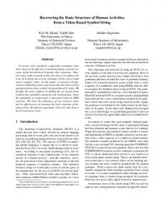
this bunch, rises to about .40. The third dimension picks up the relations with Russia scale, and more weakly, the defense spending scale. With the third dimension, the r-square for the Russia scale rises to .70. The five-point tax cut scale doesn't fit well with any of the three dimensions. The problem with it is that everyone appears to favor tax cuts. If conventional t-tests were applied using the estimated standard errors, then all the w s for the first dimension, seven of the fourteen w s for the second dimension, and only two of the fourteen 3 s for the third dimension are statistically significant. If Y were known with certainty, then the standard errors for the 6;s would be 1.3564= .128, which for reasons explained above, is, on average, smaller than the bootstrapped standard errors. The standards errors for the 6,'s and 6,'s under the certainty assumption would be .I44 and ,145, respectively. Both are much smaller than the bootstrapped standard errors. Figure 1 shows the distribution across the first basic dimension of the Carter, Reagan, and Anderson voters for the 1980 election. The Carter and Reagan voters are differentiated ideologically with the center splitting between them. Anderson was clearly drawing his support from Carter's "territory." On a -1 to +1 scale, the mean locations for the Reagan, Carter, and Anderson voters were .165, -. 165, and -.113, respectively. The corresponding standard deviations were .229, .288, and .248. The Reagan voters were clearly more ideologically coherent than the Carter voters (the smaller standard deviation). This coherence is also reflected in the fact that a larger percentage of Reagan's voters answered all fourteen issues questions than did Carter's voters-32.1% versus 26.1%, respectively. However, fully 41.3% of Anderson's voters were informed. Given Anderson's failure to "break through" to widespread mass awareness of his candidacy and what it stood for, it is not surprising that those who did support him were more informed than other voters. Third party candidates in the United States typically attract more intense supporters as a percentage of total support than the two major parties (for a history and discussion of this point, see Sundquist 1983).

B. Fitting Together Coordinate Configurations The scaling procedure for estimating equation [I] is also a solution for what is known in psychometrics as an "orthogonal procrustes" problem (Schonemann 1966; Schonemann and Carroll 1970). Suppose the columns of X, are the scaled coordinates of individuals on the same issue scale or attribute dimension at n different times. With s inherently equal to one, @ will be the n by 1 vector of best fitting average coordinates for the indivTduals over the time span. This is so because if the elements of the coordinate matrix X, are replaced by (xij - 2j) / G j , this minimizes the sum of squares

Keith I: Poole

982

Figure 1. 1980 Voters on First Basic Dimension Number

Liberal

Conservative Reagan

Carter

Anderson

between the common elements in each pair of configurations. In effect, the m configurations are "squeezed together" as tightly as possible when they are transformed by (xij 1 G j , and the mean configuration around which they are "squeezed" or "targeted" is \ir . In order to test the model's performance as an orthogonal procrustes procedure, the combined set of W-NOMINATE (Poole and Rosenthal 1997) scores for members of the House and Senate for Congresses 75 to 104 (1937 through December, 1995) will be fitted together. The scores range from -1.0 to +1.0 and are based upon all the nonunanimous roll call votes taken during a Congress. The first dimension score measures the degree of liberalism/ conservatism of the legislator. It is possible to analyze the House and Senate W-NOMINATE scores together because 151 individuals served in both chambers for at least five Congresses during the 1937 to 1995 period. If legislators are assumed to maintain a fixed position on the underlying 1iberaVconservativebasic dimension when they move from the House to the Senate or vice versa, then the model shown in equation [IB] and the procedure shown in Table 1 can be modified so that a joint House and Senate configuration can be estimated.

ej)

983


In this application, Xo has thirty columns-one for each Congress-and a row for each person serving in at least five Congresses from 1937 to 1995. A total of 1,431 legislators served in at least five Congresses during this period-1,106 in the House only, 174 in the Senate only, and 151 served in both chambers. To see how this is accomplished, let n, be the number of legislators who served in the House only, let nu be the number of legislators who served only in the Senate, nb be the number of legislators who served in both chambers, and let \Vh, \Vu, and W b be the corresponding vectors of underlying liberal1 conservative basic coordinates of length n,, nu, and nb, respectively. This produces the equations: r

i

where XOhand Xo, are the n, + n, by m and nu + n, by m matrices of W-NOMINATE scores for the House and Senate, respectively. The procedure to estimate equations [17A] and [17B] is the same as that shown in Table 1, only now some booeeeping i~~necessary when the legislator coordinates are estimated. Given Wh, , W, , and i, , the coordin!te for a legislator who only served in the House can be estimated by using Wh, and in equation [6]; similarly, if a legislator served only in the Senate, then w U ,and 6, are used in equation [6]. If a legislator served in both chambers then a W matrix can be formed from wh,and W, , by using the rows corresponding to the chamber served in and a c vector can be conby using the entries corresponding to the chamber structed from &,and served in. Given estimates of the legislator coordinates, $ , -u $ , and re-h spectively, then it is a simple matter to estimate Wh and ch and W, and c, using equation [7]. This process can be repeated as many times as desired. The results are shown in Table 5. Table 5 shows the fit statistics for the W-NOMINATE first dimension scores for the House and Senate in the same fashion as Table 4. Because this is overlapping generations data, the requirement of five entries in each row of Xo reduced the number of members included in the analysis from the early and late Congresses (the n j ) That is, to be included in the column for the 75th Congress (the first column of Xo ), a member would have had to serve five Congresses beginning with the 75th Congress (service does not have to be consecutive). In contrast, to be included in the column for the 85th Congress, a member could have served in the 81st through the 85th, or

eh

ch,

e,

9,

Table 5B. Fit Statistics by Congress for Combined House and Senate W-NOMINATE Scores (continued) Senate Congress

"j

94

116

95

113

96

115

97

111

98

113

99

110

100

105

101

95

102

91

103

78

104

69

2, 0.045 (0.024) 0.075 (0.020) 0.009 (0.025) 0.059 (0.030) -0.072 (0.025) -0.060 (0.023) -0.163 (0.023) 4.112 (0.021) -0.124 (0.024) -0.141 (0.022) -0.007 (0.033)

House j

1.684 (0.051) 1.739 (0.084) 1.875 (0.080) 1.925 (0.051) 1.861 (0.067) 1.828 (0.066) 1.952 (0.054) 1.81 1 (0.055) 1.969 (0.057) 2.010 (0.089) 2.492 (0.096)

R2

"j

'j

,912

386

,914

377

.93 1

382

,928

382

,949

415

,950

412

,966

420

.972

392

,973

360

,954

264

.945

219

0.138 (0.015) 0.088 (0.016) 0.017 (0.016) -0.053 (0.017) 4.024 (0.019) -0.030 (0.018) 4.069 (0.0 18) -0.183 (0.0 18) -0.056 (0.019) -0.094 (0.019) 0.050 (0.023)

j

1.538 (0.040) 1.766 (0.048) 1.790 (0.051) 1.771 (0.047) 1.935 (0.045) 1.786 (0.047) 1.691 (0.044) 1.734 (0.045) 1.858 (0.047) 1.809 (0.046) 2.196 (0.058)

R2 .910 ,937 .952 ,958 .965 .961 .961 ,966 .961 .950 .951


987

the 85th through the 89th. Finally, to be included in the 104th column, a member would have had to serve in five Congresses ending with the 104th. The overall fit of the model stated in equation [17] is a respectable rsquare of .918 indicating that members of Congress are very stable in their location on the liberal/conservative dimension over time. The standard errors were computed using the same approach as that for the issue scale data shown in Table 4. If conventional t-tests were applied using the estimated standard errors (recall that the "certainty" standard errors are smaller than the bootstrapped standard errors), all the w s for both the House and Senate are statistically significant. The missing data in this example are qualitatively different from the missing data in the 1980 issue scale example. In the issue scale example, there is missing data because of nonresponses. Here the data is missing simply because legislators were not in Congress. Both are treated the same by the scaling procedure. Substantively, if a respondent does not understand a question and does not give an answer, then equation [I] may not be the appropriate model for that respondent's answers. There is no easy solution for this problem. However, if the amount of missing data is low as it is in 1980 issue scale application, it is probably not a serious problem. Given the $'s for members serving in at least five Congresses, coordinates for members serving in less than five Congresses can be estimated using the 9 s and 6's by applying the transformation: (xij - Cj) / G j and taking the average over the total number of Congresses served. That is:

where mi is the total number of Congresses served and ranges from one to four, and the 9 s and 6's can be a combination of those from the House and the Senate if the member served in both chambers. Figure 2 shows the means for the political parties over the 1937 to 1995 period combining the $i's estimated by the procedure and the $i's from equation [IS]. The two chambers are very similar in their patterns over time. In the latter part of the New Deal, voting on minimum wages opened up a split between the northern and southern wings of the Democratic party. During World War 11, voting on issues related to the right of Blacks to vote in federal elections exacerbated the split (Poole and Rosenthal 1997, chap. 5). Southern Democrats move to the right in both chambers until just after the Civil Rights era of the mid to late 1960s and then begin moving back to the left during the 1970s and 1980s. Republicans shift to the left from the late

Keith 7: Poole

Figure 2A. House of Representatives 1st Dimension of Joint Space

Figure 2B. Senate 1st Dimension of Joint Space 0.4

? .-w

E 3

0.2

3 0

-

$ -0.2


989

1940s and then reverse course after the Civil Rights era. Republicans in both chambers have been moving to the right since the late 1970s (Poole and Rosenthal 1997; McCarty, Poole, and Rosenthal 1997). Note that because each member is assumed to have the same position throughout his career, these shifts in the various party means are due to replacement not conversion. The correlation between the chamber means is .90 indicating that whatever forces are at work in American politics tend to work on both chambers equally regardless of their very different constituencies, terms, and internal rules and procedures. Viewed over a long period of time, there is no pat answer to the question: is the Senate more liberal than the House.21The corresponding correlations for Republicans, northern Democrats, and southern Democrats are .81, .84, and .76, respectively.

6. Conclusion The scaling procedure shown in this paper performs, in effect, a singular value decomposition of a rectangular matrix of real elements with missing entries. In contrast to existing techniques such as factor analysis which work with a correlation or covariance matrix computed from the data matrix, the scaling procedure shown here analyzes the data matrix directly without any intervening transformations of the original data. It is a general-purpose tool that can be used to estimate latent/unobservable dimensions underlying a set of manifest/observable variables or as a method to obtain an Eckart-Young lower-rank approximation matrix of a matrix with missing entries. Monte Carlo tests show that the procedure does a good job of reproducing the missing elements of a matrix even at high levels of error and missing data. Manuscript submitted 21 January 1997.

Final manuscript received 16 September 1997.

APPENDIX A The partial derivatives of equation [4] are

?'See Froman (1971) and Kernel1 (1973) for a discussion of House-Senate differences.

990

Keith 7: Poole

where n, means that the total of the summation over i may vary from 2m to n depending upon how many entries there are in the ith column of Xo . To see that y = , note that

and -all =

The first term on the right is equal to zero because i=1 j=1

and the third and fourth terms are equal to zero because

j=1 i=1

ac

0,

Z vik= 0 . Hence, the sec-

ond term, 2nyk , must equal zero. Therefore, yk = 0 because n > 0. To see that the Q's are all zero, consider the two equations:

and

because

=

the first term in both equations are identical. Hence

Qkhhh= -Qkhhh. NOW,since hh is the hth singular value in A and by assumption the s singular values in A are greater than zero, then mkh = 0.

mkh =

-@kh

which is possible only if


99 1

APPENDIX B To maximize the number of positive elements in the m by m covariance matrix

a vector of plus and minus ones must be found so that when they are placed on the diagonal of an m by m diagonal matrix A*, the number of positive elements in the m by m matrix:

will be maximum. For example, suppose the covariance matrix is

Clearly, changing the signs of the fourth column and row will reduce the number of negative elements in the matrix. That is,

Any further changes of the signs of the columns/rows will increase the number of negative elements in the matrix. Note that another solution for the diagonal of A* is (-1,1,1,1). This also reduces the number of negative elements to four. A simple algorithm to produce a diagonal for A* is to find the row in the covariance matrix with the most negative elements and change its sign and that of the conesponding column (if no row has more than (m - 1)/2 negative elements, than no sign changes are necessary). This process is then repeated. The row with the next most negative elements is found and its sign is changed. This process can be continued until all rows have (m - 1)/2 or less negative entries.

REFERENCES Aldrich, John, and Richard D. McKelvey. 1977. "A Method of Scaling with Applications to the

1968 and 1972 Presidential Elections." American Political Science Review 71: 111-30.

Brady, Henry. 1990. "Traits versus Issues: Factor versus Ideal-Point Analysis of Candidate Ther-

mometer Ratings." Political Analysis 2:97-129.

992

Keith 7: Poole

Cahoon, Lawrence, Melvin J. Hinich, and Peter C. Ordeshook. 1978. "A Statistical Multidimensional Scaling Method Based on the Spatial Theory of Voting." In Graphical Representation oj Multivariate Data, ed. P. C. Wang. New York: Academic Press. Carroll, J. Douglas. 1972. "Individual Differences and Multidimensional Scaling." In Multidimensional Scaling, ed. Roger N. Shepard, A. Kimball Romney, and Sara Beth Nerlove. New York: Seminar Press. Carroll, J. Douglas, and Jih-Jie Chang. 1970. "Analysis of Individual Differences in Multidimensional Scaling Via an N-way Generalization of "Eckart-Young" Decomposition." Psychometrika 35:283-319. Converse, Phillip E. 1964. "The Nature of Belief Systems in Mass Publics." In Ideology and Discontent, ed. David E. Apter. New York: Free Press. Coombs, Clyde. 1964. A Theoty of Data. New York: John Wiley. Eckart, Carl, and Gale Young. 1936. "Thz Approximation of One Matrix By Another of Lower Rank." Psychometrika 1:211-18. Enelow, James, and Melvin J. Hinich. 1984. The Spatial Theory of Voting. New York: Cambridge University Press. Enelow, James, and Melvin J. Hinich. 1994. "A Test of the Predictive Dimensions Model in Spatial Voting Theory." Public Choice 78:155-69. Feldman, Stanley, and John Zaller. 1992. "Political Culture of Ambivalence: Ideological Responses to the Welfare State." American Journal ofPolitica1 Science 36:268-307. Froman, Lewis A,, Jr. 1971. "Differences Between the House and Senate." In Readings On Congress, ed. Raymond Wolfinger. Englewood Cliffs, NJ: Prentice-Hall. Gleason, Terry C., and Richard Staelin. 1975. "A Proposal for Handling Missing Data." Psychometrika 40:229-52. Groseclose, Tim, Steven D. Levitt, and James M. Snyder, Jr. 1997. "An Inflation Index For ADA Scores." Ohio State University. Typescript. Hinich, Melvin J., and Michael Munger. 1994. Ideology and the Theory of Political Choice. Ann Arbor, MI: University of Michigan Press. Hinich, Melvin J., and Michael Munger. 1997. Analytical Politics. New York: Cambridge University Press. Hinich, Melvin J., and Walker Pollard. 1981. "A New Approach to the Spatial Theory of Electoral Competition." American Journal of Political Science 25:32341. Horst, Paul. 1963. Matrix Algebra for Social Scientists. New York: Holt, Rinehart and Winston, Inc. Jacoby, William. 1993. "Testing the Effects of Paired Issue Statements on the Seven-Point Issue Scales." Political Analysis 5:61-112. Johnson, Richard M. 1963. "On a Theorem Stated by Eckart and Young." Psychometrika 28:259-63. Keller, Joseph B. 1962. "Factorization of Matrices by Least-Squares." Biometrika 49:23942. Kernell, Sam. 1973. "Is the Senate More Liberal than the House?' Journal ofPolitics 35:332-63. Lawson, Charles L., and Richard J. Hanson. 1974. Solving Least Squares Problems. Englewood Cliffs, NJ: Prentice-Hall Inc. MacRae, Duncan. 1970. Issues and Parties in Legislative Voting: Methods of Statistical Analysis. New York: Harper and Row. McCarty, Nolan M., Keith T. Poole, and Howard Rosenthal. 1997. "Income Redistribution and the Realignment of American Politics." AEI Studies on Understanding Economic Inequality. Washington, DC: AEI Press. Ordeshook, Peter C. 1976. "The Spatial Theory of Elections: A Review and a Critique." In Party Identijication and Beyond ed. Ian Budge, Ivor Crewe, and Dennis Farlie. New York: Wiley. Poole, Keith T. 1997. "How to Use the Black Box." GSIA, Carnegie-Mellon University. Typescript. Poole, Keith T., and Howard Rosenthal. 1997. Congress: A Political-Economic Histoty ofRoll Call Voting. New York: Oxford University Press.


993

Rabinowitz, George. 1974. Spatial Models of Electoral Choice: An Empirical Analysis. Chapel Hill, NC: Institute for Research in Social Science. Rusk, Jerrold, and Herbert Weisberg. 1972. "Perceptions of Presidential Candidates." Midwest Journal ofPolitical Science 16:388-410. Schonemann, Peter H. 1966. "A Generalized Solution of the Orthogonal Procrustes Problem." Psychometrika 3 1: 1-10. Schonemann, Peter H. 1970. "On Metric Multidimensional Unfolding." Psychometrika 35:349-66 Schonemann, Peter H., and R. M. Carroll. 1970. "Fitting One Matrix to Another Under Choice of a Central Dilation and Rigid Motion." Psychometrika 35:245-56 Sundquist, James L. 1983. Dynamics ofthe Party System. Washington, DC: Brookings Institution. Takane, Yoshio, Forrest W. Young, and Jan de Leeuw. 1977. "NonMetric Individual Differences Multidimensional Scaling: An Alternating Least Squares Method with Optimal Scaling Features." Psychometrika 42:7-67. Van de Geer, John P. 1971. Introduction to Mziltivariate Analysis for the Social Sciences. San Francisco: W. H. Freeman and Company. Weisberg, Herbert, and Jerrold Rusk. 1970. "Dimensions of Candidate Evaluation." American Political Science Review 64: 1167-85.