Rectangular Schroder Parking Functions Combinatorics

arXiv:1603.09487v1 [math.CO] 31 Mar 2016

¨ RECTANGULAR SCHRODER PARKING FUNCTIONS COMBINATORICS JEAN-CHRISTOPHE AVAL AND FRANC ¸ OIS BERGERON

Abstract. We study Schr¨ oder paths drawn in a (m, n) rectangle, for any positive integers m and n. We get explicit enumeration formulas, closely linked to those for the corresponding (m, n)-Dyck paths. Moreover we study a Schr¨oder version of (m, n)parking functions, and associated (q, t)-analogs.

Contents 1. Introduction 2. Schr¨ oder paths 3. Constant term formula 4. Schr¨ oder Parking functions References

1 2 10 11 12

1. Introduction Schr¨oder numbers (1, 2, 6, 22, 90, 394, 1806, . . . ; sequence A006318 in [22]) enumerate Schr¨oder paths, defined as paths from (0, 0) to (n, n) made of steps (1, 0), (0, 1) and (1, 1), that never go strictly below the diagonal. These paths may be seen as a generalization of Dyck paths (for which only the first two types of steps are allowed), which are enumerated by Catalan numbers. The aim of this work is to investigate properties of such paths embedded not into a square (n, n), but into a rectangle (m, n). Partial results are already known, in the case where m and n are coprime, in particular when m = rn + 1, which reduces to mn = n [23]. In the present article, (see Proposition 1) we obtain a generating series formula, in the general case (no coprimality required). As we shall see, the result, as well as the method, is closely related to the case of Dyck paths studied in [2]. Moreover, we study Schr¨oder parking functions, defined as labeled rectangular Schr¨oder paths, and investigate q− and (q, t)−analogs of our enumeration formulas, in which the parameter q takes into account the area between the path and the diagonal (a precise definition is given at Subsection 2.6). Date: April 1, 2016. This work was supported by NSERC-Canada. 1

2

J.-C. AVAL AND F. BERGERON

¨ der paths 2. Schro 2.1. Schr¨ oder polynomials. Although the general notion of (m, n)-Schr¨oder paths considered here seems to be new, the special case of m = rn + 1 has been considered in [23]. The “classical case” corresponds to m = n. In this case, Schr¨oder polynomials, given by the following formula    n X 1 n n+k k Sn (y) := y , (1) k+1 k n k=0 with S0 = 1, have a long and interesting history. One of the known facts is that the (k) coefficient of y k , denoted Sn , enumerates “Schr¨oder paths” having k “diagonal steps” (relevant definitions are recalled below). The case k = 0 corresponds to the usual notion of “Dyck paths”, which are well-known to be counted by Catalan numbers   1 2n (0) Sn = . n+1 n Small values of these polynomials are S1 (y) S2 (y) S3 (y) S4 (y) S5 (y)

= = = = =

1 + y, 2 + 3 y + y2, 5 + 10 y + 6 y 2 + y 3 , 14 + 35 y + 30 y 2 + 10 y 3 + y 4 , 42 + 126 y + 140 y 2 + 70 y 3 + 15 y 4 + y 5 .

We consider a “rectangular” generalization of these polynomials, parametrized by pairs (m, n), with the classical case corresponding to m = n. Just as it transpires in the analogous situation for Dyck paths, the case when m and n are coprime is somewhat simpler. To make this more apparent notation-wise, we usually assume that (m, n) = (ac, bc), with (a, b) coprime. Hence c is the greatest common divisor of m and n. Thus the (a, b)-case corresponds to the coprime situation. We recall that the number of (a, b)-Dyck paths, is simply given by the formula   1 a+b . a+b a The general case is probably best coined in generating series format as ! X X 1 ja + jb z j Cac,bc z d = exp . (2) a ja j j>1 d≥0 The proof of this formula, going back to 1954, is due to Bizley [11], who attributes it to Grossman [17]. 2.2. Schr¨ oder path. We define (m, n)-Schr¨ oder paths to be sequences of points (x, y) in N × N such that • they begin with (0, 0) and end with (m, n),

SCHR¨ oDER COMBINATORICS

Row labels

3

Row areas

0

3

1

6

2

6

3

4

4

3

5

4

6

2

7

1

8

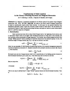
0 Figure 1. The (12, 9)-Schr¨oder path 000022237.

• all such that my − nx ≥ 0, and • with the next point obtained by either an up, diagonal, or right step. These steps respectively correspond to adding (0, 1), (1, 1) or (1, 0) to a point (x, y). Alternatively, the path could readily be encoded as a word in the letters u, d and r, (k) with obvious conditions. We shall denote by Sm,n the set of (m, n)-Schr¨oder paths with exactly k diagonal steps. Given m and n, for each point (u, v) in N × N, we define its (m, n)-offset to be d(u, v) := mv − nu.

(3)

Thus, we respectively have d(u, v) > 0, d(u, v) = 0 and d(u, v) < 0, according to the case of (u, v) sitting above, on, or below the diagonal my = nx. The low points of (any) path are those of minimal off-set (excluding the origin (0, 0)). Thus, if a path goes below the diagonal, its low-points are those that sit farthest to the “south-east” (this rather depends on m and n) of the path. 2.3. Sequence encoding. It is often practical to bijectively encode our paths in terms of a sequences a0 a1 · · · an−1 , one ai for each up or diagonal step on the path, reading them from top to bottom. For each up step, we set ai = k (resp. ai = k for diagonal steps), where k is the number of entire “cells” that lie to the left of the unique up (or diagonal) step at height n − i. The ai are said to be the parts of α. An ai of the form k is said to be barred. In this encoding, α = a0 a1 · · · an−1 corresponds to an (m, n)-Schr¨oder path if and only if (1) a0 ≤ a1 ≤ . . . ≤ an−1 , (with the order 0 < 0 < . . . k < k), (2) if ai = k, then necessarily ai < ai+1 , and (3) for each i, we have ai ≤ bi m/nc.

4

J.-C. AVAL AND F. BERGERON

Each unbarred k, between 0 and m, occurs with some multiplicity1 nk in a path α. Removing 0-multiplicities, we obtain the (multiplicity) composition γ(α) of the sequence α, reading these multiplicities in increasing values of k. For example, γ(001112444) = (1, 2, 1, 2). Clearly γ(α) is a composition of n − k, where k stands for the number of diagonal steps in α. The parts of γ(α) may be understood as the lenghts of risers in the path. These are maximal sequences of consecutive up-steps. Any (m, n)-Schr¨oder paths may be obtained by either barring or not the rightmost part of a given size in the analogous word encoding of an (m, n)-Dyck path. As we will see this makes the enumeration of Schr¨oder easy, once we setup the right tools. 2.4. Symmetric function weight. As we will come to see more clearly later, it is interesting to consider a weighted enumeration of Schr¨oder paths, with the weight lying in the degree graded ring M Λ= Λd d≥0

of symmetric “functions” (polynomials in a denumerable set of variables x = x1 , x2 , x3 , . . .). Recall that the degree d homogeneous component Λd affords as a linear basis the set {eµ (x) | µ ` d}, of elementary symmetric functions, with eµ (x) := eµ1 (x)eµ2 (x) · · · eµ` (x) for µ = µ1 µ2 . . . µ` running over the set of partitions of d. In turn, each factor ek (x) is characterized by the generating function identity Y X ek (x)z k = (1 + xi z). (4) k≥0

i≥1

with e0 (x) := 1. It easily follows that ek (x + y) = ek (x) + ek−1 (x) y,

(5)

where x + y means that we add a new variable y to those occurring in x. With these notions at hand, we now simply set X Sm,n (x; y) := α(x) y diag(α) , with α

α(x) :=

Y

ek (x),

(6)

k∈γ(α)

and where the sum is over the set of (m, n)-Schr¨oder paths α, with diag(α) denoting the number of diagonal steps in α. Likewise, we denote by X (k) Sm,n (x) := α(x), (7) diag(α)=k 1possibly

equal to 0.

SCHR¨ oDER COMBINATORICS

5

the symmetric function enumerator of (m, n)-Schr¨oder paths with exactly k diagonal P (k) steps, so that Sm,n (x; y) = k Sm,n (x) y k . For example, we have, S1,1 (x; y) = e1 (x) + y, S2,2 (x; y) = (e11 (x) + e2 (x)) + 3 e1 (x) y + y 2 , S3,3 (x; y) = (e111 (x) + 3 e21 (x) + e3 (x)) + (6 e11 (x) + 4 e2 (x))y + 6 e1 (x)y 2 + y 3 . Observe that, for all r and n, we have Srn+1,n (x; y) = Srn,n (x; y),

(8)

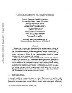
since the last step of (rn + 1, n) must necessarily be a right step, and the coprimality of rn + 1 and n that staying below the (rn + 1, n)-diagonal insures as well that we stay below the (rn, n)-diagonal. Hence we get the same set of paths. To make some expressions more compact, we shall use “plethystic notation”, recalling that we have X pν (x) en [m x] := (−m)`(ν) , (9) z ν ν`n with a, j and m considered as “constants” for the purpose of plethysm. For any partition ν of n, of length `(ν), we set zν := 1d1 d1 !2d2 d2 ! . . . ndn dn !, where di is the number of copies of the part i in ν. 2.5. Main result. Proposition 1. The generating function of rectangular Schr¨oder polynomials is given by the following equation: ! j X X z Sad,bd (x) z d = exp . (10) ejb [ja (x + y)] aj j≥1 d≥0 Proof. The proof is inspired from Bizley’s original proof [11] (see also [2]). For fixed (k) m, n and k, we consider two classes of lattice paths. The first class is the class Sm,n of (m, n)-Schr¨oder paths with exactly k diagonal steps. The second class, which is denoted (k) by Bm,n , consists of similar paths, with same start and end points, finishing with either a diagonal or a horizontal step, but without the above diagonal condition. Naturally, (k) Bm,n stands for the (clearly disjoint) union of the sets Bm,n . See Figure 2. We extend to such paths the symmetric function weight (6) previously only considered (k) on Sm,n , and naturally set X X (k) (k) Bm,n (x) := α(x), and Bm,n (x; y) := Bm,n (x) y k , (11) α

k (k)

with the first sum over the α’s in Bm,n . Using the multinomial coefficient notation   n n! := , for µ = (µ1 , µ2 , . . . , µk ) ` d ≤ n. µ (n − d)!µ1 !µ2 ! · · · µk !

6

J.-C. AVAL AND F. BERGERON

(3)

Figure 2. An element of B12,9 with 2 low points. Let us prove that (k) Bm,n (x)

X m m  = eν (x). k dν ν`n−k

(12)

(k)

To see this, we observe that an element α of Bm,n is fully characterized by the following data • A partition ν of n − k which describes the ordered sequence of lengths for vertical risers, giving γ(α); • The
positions of the k diagonal steps among m, hence enumerated by the binomial m ; k
• The positions of the parts of ν, counted by the binomial dmν . (k,`)

Using a Bizley-like argument, exploiting the notion of low points, we denote by Sm,n (k,`) (k) (k) and Bm,n the subsets of Sm,n and Bm,n consisting of paths with exactly ` low points (i.e. those having most negative offset, see (3)). Continuing with the logic of our previous (k,`) (k,`) notations, we denote by Sm,n (x) and Bm,n (x) the corresponding weighted sums. We briefly recall the notion of rotation and refer to [11, 2] for a detailed presentation. Let us (k,`) consider an element α of Bm,n . We may cut α at any of its ` low points, and transpose the two resulting path components. This operation preserves the number of low points, as well as the risers of α. By this rotation principle, we have a set bijection (k,`) (k,`) Sm,n × [m] ' Bm,n × [`],

hence it follows that X1 `

`

(k,`) Sm,n (x) =

1 X (k,`) 1 (k) Bm,n (x) = Bm,n (x). m ` m

(13)

SCHR¨ oDER COMBINATORICS

7

Summing over k gives: X1 1 X (k) 1 (k,`) (x)y k = Sm,n Bm,n (x)y k = Bm,n (x; y). ` m k m `,k

(14)

Next, we recall the following expansion of (9) in terms of elementary symmetric functions X m en [m x] = eν (x), (15) d ν ν`n with dν the partition giving the (ordered) multiplicities of the parts of ν. Thus, using (12) and (15) we calculate that X X m m  k Bm,n (x; y) = y eν (x) k d ν k ν`n−k n   X m = en−k [m x] y k k k=0 =

n X

en−k [m x] ek [m y]

k=0

= em [n(x + y)]. We may thus rewrite (14) as: X1 `

`,k

(k,`) Sm,n (x; y) =

(16)

1 em [n(x + y)], m

(17)

P (k,`) (∗,`) which is the crux of the proof. We may then set: Sm,n (x, y) := k Sm,n (x, y) and observe that X (∗,1) (∗,`) (∗,1) (∗,1) Sac,bc (x, y) = Sac1 ,bc1 (x, y) Sac2 ,bc2 (x, y) · · · Sack ,bck (x, y) (18) γ|=t c

where the sum is over length ` compositions γ = (c1 , c2 , . . . , ct ) of c. In other terms, if we set ∞ X (∗,1) (∗,1) Sa,b (x, y, z) := Saj,bj (x, y) z j , j=1


` (∗,`) (∗,1) then Sac,bc (x, y) is the coefficient of z c in Sa,b (x, y, z) . Thus (17) means that y)] is the coefficient of z c in − log(1 − (∗,1) Sa,b (x, y, z)

(∗,1) Sa,b (x, y, z))),

X

∞  X 1 c = 1 − exp − eac [bc(x + y)] z . ac c=1

Sad,bd (x) z d =

d≥0

which, together with (19) gives(10).

eac [bc(x+

whence



We observe that

1 ac

(19)

1 (∗,1)

1 − Sa,b (x, y, z) 

8

J.-C. AVAL AND F. BERGERON

For example, for any a and b coprime, we get 1 Sa,b (x + y) = eb [a (x + y)], a

(20)

S2a,2b (x + y) =

1 1 e2b [2a (x + y)] + 2 eb [a (x + y)]2 , 2a 2a

S3a,3b (x + y) =

1 1 1 e3b [3a (x + y)] + 2 eb [a (x + y)] e2b [2a (x + y)] + 3 eb [a (x + y)]3 . 3a 2a 6a (22)

(21)

Recall from [2] that we have a Bizley-like formula for the symmetric function enumeration X Cm,n (x) := α(x), (23) diag(α)=0

of (m, n)-Dyck paths, namely ! j z , Cad,bd (x) z d = exp ejb [ja x] aj j≥1 d≥0

X

X

(24)

This gives us the following formulation of Proposition 1. Corollary 2. For all m and n, we have Sm,n (x; y) = Cm,n (x + y).

(25)

Remark 3. We proved (25) by computation of both sides, and comparison. It would be interesting to get this equality directly by a suited interpretation of the substitution x 7→ x + y. As a special case, recalling that we assume a and b to be coprime, we have: 1 Sa,b (x; y) = eb [a (x + y)]. (26) a Moreover, we may write the coefficient of y k in (26) as the following integer coefficient linear combination of the eν (x): X 1 a a  (k) Sa,b (x) = eν (x). (27) a k d ν ν`b−k P Since heµ (x), j≥0 ej (x)i = 1 for all partition µ, we immediately get D E X (k) (k) Sa,b = Sa,b (x), ej (x) . j≥0

Otherwise stated, for a and b coprime, (k) Sa,b

X 1 a a  = . a k dν ν`b−k

(28)

SCHR¨ oDER COMBINATORICS

9

In particular, in view of (8), this covers the classical case (m = n) as well as the generalized version (m = rn) of [23]. One also deduces from Proposition 2 the following generalization of a result of Haglund [15]. Proposition 4. For all m and n, D E (k) = Cm,n (x), en−k (x)hk (x) Sm,n

(29)

where h−, −i stands for the usual scalar product on symmetric function2. Proof. We start by recalling the symmetric function identity X f (x + y) = y k h⊥ k f (x),

(30)

k≥0

where h⊥ k stands for the dual of the operator of multiplication by hk (x) with respect to the symmetric function scalar product. It follows directly from (25) that E D X X (k) k ek (x) , Sm,n y = Cm,n (x + y), k≥0

k

=

DX

=

D

=

XD

y k h⊥ k Cm,n (x),

X

E ej (x) ,

j≥0

k≥0

Cm,n (x),

X

y k hk (x)

k≥0

X

E ej (x) ,

j≥0

E Cm,n (x), hk (x)en−k (x) y k .

k≥0

The last equality comes from the fact that Cm,n (x) is homogeneous of degree n, hence all terms of the wrong degree vanish in the scalar product. Evidently we get the announced result by comparing same degree powers of y in both sides of the identity obtained.  (r)

2.6. Area enumerator. The ith row area of a path α in Sn , is the integer areai (α) := bi m/nc − |ai |,

(31)

where we set |k| := k. Summing over all indices i, between 1 and n, we get the area of α: n−1 X area(α) := areai (α). (32) i=0

This generalizes to (m, n)-Schr¨oder paths a notion of area on Schr¨oder paths introduced for the case m = n in [12] (and further studied by [3]). Following the presentation of [15], this may also be understood as the number of “upper” triangles lying above the 2For

which hpµ , pν i = zµ δµ,ν

10

J.-C. AVAL AND F. BERGERON

path and below the diagonal line (as illustrated in Figure 1). These triangles are also called area triangles. We have the area q-enumerator symmetric function X Sm,n (x; y, q) := α(x) q area(α) y diag(α) . (33) α

Keeping up with our previous notation conventions, we also set X X (k) Sm,n (q) := q area(α) , and Cm,n (x; q) := diag(α)=k

α(x) q area(α) .

(34)

diag(α)=0

Observing that the area is independent of whether elements are barred or not, we deduce from Corollary 2 that Corollary 5. For all m and n, we have Sm,n (x; y, q) = Cm,n (x + y; q),

(35)

D E (k) Sm,n (q) = Cm,n (x; q), en−k (x)hk (x) .

(36)

and

From a result of [18], it follows that Crn+1,n (x; q) = Crn,n (x; q) = ∇r (en ) t=1 , where ∇ is a Macdonald “eigenoperator” introduced in [6]. By this, we mean that its eigenfunctions are the (combinatorial) q, t-Macdonald polynomials. Thus, a special instance of (36) may be formulated as D E (k) Srn,n (q) = ∇r (en ) t=1 , en−k (x)hk (x) . (37) In this way, we get back the case t = 1 of Proposition 1 in [15].

3. Constant term formula The following constant term formula adds an extra parameter to our story. We conjecture that it corresponds to a (q, t)-enumeration of (m, n)-Schr¨oder parking function, with t accounting for a correctly defined “dinv”-statistic. ! m m Y (zi − zj )(zi − qt zj ) 1 Y zi (1 + y zi ) 0 Ω (x; zi ) , Sm,n (x; y, q, t) := CTzm ,...,z0 zm,n i=1 zi − q zi+1 (z − qz )(z − tz ) i j i j j=i+1 (38) P Qn−1 where Ω0 (x; z) := k≥0 ek (x) z k , and zm,n := i=0 zbim/nc . We recall that some care must be used in evaluating multivariate constant term expressions. Indeed, the order in which successive constant terms are taken does have an impact on the overall result. This is why, in the above formula, the indices appearing after “CT” specify that this

SCHR¨ oDER COMBINATORICS

11

should be done starting with zm , and then going down to z0 . For example, we have S2,2 (x; y, q, t) = (s2 + (q + t) s11 )+(q + t + 1) s1 y + y 2 , S2,3 (x; y, q, t) = (s21 + (q + t) s111 )+(s2 + (q + t + 1)s11 ) y + s1 y 2 , S2,4 (x; y, q, t) = (s22 + (q + t) s211 + (q 2 + qt + t2 ) s1111 ) +((q + t + 1) s21 + (q 2 + qt + t2 + q + t) s111 ) y +(s2 + (q + t) s11 ) y 2 . We underline that formula (38) is simply the evaluation at x + y of a similar formula conjectured in [21] in relation with (m, n)-parking functions. More precisely, it is conjectured in the mentioned paper, that ! m m Y 1 Y zi (zi − zj )(zi − qt zj ) 0 Ω (x; zi ) , Cm,n (x; q, t) := CTzm ,...,z0 zm,n i=1 zi − q zi+1 (zi − qzj )(zi − tzj ) j=i+1 (39) from which it is clear that (38) follows, since Ω (x + y; zi ) = (1 + y zi ) Ω (x; zi ). One may readily show that the specialization at t = 1 of the right-hand side of (38) does indeed give back our previous Cm,n (x + y; q) = Sm,n (x; y, q), since the relevant constant term formula is shown to hold in [8]. 0

0

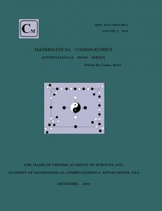
This, together with the results and conjectures that appear in [8], opens up a lot of new avenues of exploration. In particular, we may obtain explicit candidates for the (q, t)enumeration of special families of (m, n)-Schr¨oder paths (say with return conditions to the diagonal), by the simple device of evaluating at x + y analogous symmetric function formulas for (m, n)-Dyck paths. Several questions regarding this are explored in [4]. ¨ der Parking functions 4. Schro An (m, n)-Schr¨ oder parking function is a bijective labeling of the up steps of a (m, n)-Schr¨oder path α by the elements of {1, 2, . . . , n − diag(α)}. One further imposes the condition that consecutive up steps of same x-coordinate have decreasing labels reading them from top to bottom. The path involved in this description is said to be the shape of the parking function. For α an (m, n)-Schr¨oder path, we denote by P(α) the set of parking function having shape α. When diag(α) = 0, we get the “usual” notion of parking functions of shape α (an (m, n)-Dyck path). The (m, n)-Schr¨oder parking functions may be understood as preference functions, with some of the parking places being closed to parking (these correspond to diagonal steps). For f ∈ P(α), we denote by areai (f ) the row area for the ith row of the shape of f . Figure 3 gives an example of a parking function of shape 000011223. As we did for paths, we consider the (m, n)-Schr¨oder parking function polynomial X X (k) k Pm,n (y, q) = Pm,n y := |P(α)| q area(α) y diag(α) . (40) k

It is easy to derive from Corollary 5 that

α

12

J.-C. AVAL AND F. BERGERON

4 5 3 7 6 2 1 Figure 3. A Schr¨oder parking function. Corollary 6. For all m and n, we have  Pm,n (y, q) = Cm,n (x + y; q),

 1 . 1 − p1 (x)

Equivalently, for all k D E (k) Pm,n (q) = Cm,n (x; q), p1 (x)n−k hk (x) ,

(41)

It follows from this, and the observation preceding (37), that D E (k) r n−k Prn,n (q) = ∇ (en ) t=1 , p1 (x) hk (x) .

(42)

Also, for a and b coprime, we have (k) Pa,b

  a b−k−1 = a . k

(43)

References [1] D. Armstrong, N. Loehr, and G. Warrington, Rational Parking Functions and Catalan Numbers, arXiv:1403.1845, (2014). [2] J.-C. Aval, and F. Bergeron, Interlaced rectangular parking functions, arXiv:1503.03991, (2015). [3] E. Barcucci, A. Del Lungo, E. Pergola, and R. Pinzani, Some combinatorial interpretations of q-analogs of Schr¨ oder numbers, Ann. Comb. 3, 1999, 171–190. [4] F. Bergeron, Open Questions for operators related to Rectangular Catalan Combinatorics, 2016. [5] F. Bergeron, Algebraic Combinatorics and Coinvariant Spaces, CMS Treatise in Mathematics, CMS and A.K.Peters, 2009. [6] F. Bergeron and A. M. Garsia, Science Fiction and Macdonald Polynomials, Algebraic methods and q-special functions (L. Vinet R. Floreanini, ed.), CRM Proceedings and Lecture Notes, American Mathematical Society, 1999.

SCHR¨ oDER COMBINATORICS

13

[7] F. Bergeron, A. M. Garsia, M. Haiman, and G. Tesler, Identities and Positivity Conjectures for Some Remarkable Operators in the Theory of Symmetric Functions, Methods in Appl. Anal., 6 (1999), 363–420. [8] F. Bergeron, E. Leven, A. M. Garsia,and G. Xin, Compositional (km, kn)–Shuffle Conjectures, arXiv:1404.4616, (2014). ´ville-Ratelle, Higher Trivariate Diagonal Harmonics via generalized [9] F. Bergeron, L.-F. Pre Tamari Posets, Accepted for publication in Journal of Combinatorics. (see arXiv:1105.3738) [10] O. Bernardi and N. Bonichon, Catalan’s intervals and realizers of triangulations, Journal of Combinatorial Theory, Series A Volume 116, Issue 1 (2009), 55–75. [11] T. L. Bizley, Derivation of a new formula for the number of minimal lattice paths from (0, 0) to (km, kn) having just t contacts with the line and a proof of Grossmans formula for the number of paths which may touch but do not rise above this line, J. Inst. Actuar. 80, (1954), 55–62. [12] J. Bonin, L. Shapiro, and R. Simion, Some q-analogues of the Schr¨ oder numbers arising from combinatorial statistics on lattice paths, J. Statist. Plann. Inference 34, 1993, 35–55. ´lou, G. Chapuy, and L.-F. Pre ´ville-Ratelle, m-Tamari Intervals and [13] M. Bousquet Me Parking Functions: Proof of a Conjecture of F. Bergeron, (see arXiv:1109.2398). [14] Ph. Duchon, On the Enumeration and Generation of Generalized Schr¨ oder Words, Discrete Mathematics 225 (2000), 121–135. [15] E. S. Egge, J. Haglund, K. Killpatrick, D. Kremer, A Schr¨ oder Generalization of Haglund’s Statistic on Catalan Paths, Electronic Journal of Combinatorics 10 (2003), #R16. [16] I. Gessel, Schr¨ oder numbers, large and small, CanaDAM2009. (see Gessel.slides) [17] H. D. Grossman, Fun with lattice points: paths in a lattice triangle, Scripta Math. 16 (1950), 207-212. [18] M. Haiman, Combinatorics, symmetric functions and Hilbert schemes, In CDM 2002: Current Developments in Mathematics in Honor of Wilfried Schmid & George Lusztig, International Press Books (2003), pp. 39–112. [19] J. Haglund, M. Haiman, N. Loehr, J. Remmel, and A. Ulyanov, A Combinatorial Formula for the Character of the Diagonal Coinvariants, Duke Math. J. Volume 126, Number 2 (2005), 195-232. [20] T. Koshy, Catalan Numbers with Applications, Oxford University Press, 2009. [21] A. Negut, The Shuffle Algebra Revisited, Int. Math. Res. Notices (2014) (22): 6242–6275. doi: 10.1093/imrn/rnt156 arXiv:1209.3349, (2012). [22] N.J.A Sloane, The On-Line Encyclopedia of Integer Sequences, http://oeis.org. [23] C. Song, The Generalized Schr¨ oder Theory, Electronic Journal of Combinatorics 12 (2005), #R53, ´ de Bordeaux, 351 cours de la Libe ´ration, 33405 Talence, LaBRI, CNRS - Universite France ´partement de Mathe ´matiques, UQAM, C.P. 8888, Succ. Centre-Ville, Montre ´al, H3C De 3P8, Canada.